Gibbs Distribution and the Repairman Problem

Abstract

In this paper, we obtain weak convergence results for a family of Gibbs measures depending on the parameter $\theta >0$ in the following form $d{P}_{\theta }\left(x\right)=Z_{\theta }exp\left(-H_{\theta }\left(x\right)/\theta \right)dQ\left(x\right)$, where we show that the limit distribution is concentrated in the set of the global minima of the limit Gibbs potential. We also give an explicit calculus for the limit distribution. Here, we use the above as an alternative to Lyapunov’s function or to direct methods for stationary probability convergence and apply it to the repairman problem. Finally, we illustrate this method with a numerical example.

1. Introduction

In this paper, we study the weak convergence of a family of Gibbs probability measures via Laplace’s method ([1,2,3,4]). This method is interpreted as a weak convergence of probability measures, which was used by Hwang [5]. Yu. Kaniovski and G. Pflug [6] investigated Laplace’s method to study the limit stationary distribution of the birth and death process.

In this paper, we suppose that the Gibbs potential $H_{\theta }$ depends on a parameter $\theta$, and Q is a probability measure on the Euclidean space ${\mathbb{R}}^r$, such that it dominates $P_{\theta }$ for any $\theta$. To show the tightness of the family

$${\displaystyle \frac{d{P}_{\theta }}{dQ}\left(x\right)=Z_{\theta }exp\left(-H_{\theta }\left(x\right)/\theta \right),\theta >0,}$$

(1)

we give some additional conditions for the probability measure Q and for the limit Gibbs potential H of $H_{\theta }$ when $\theta \to 0$. Under these conditions, the limit distribution P of $P_{\theta }$, as $\theta \to 0$, is concentrated on the set of the global minima of the limit Gibbs potential, so we give an explicit calculus for the limit probability P. We use these results to prove that the stationary probability of the repairman problem converges to some probability measure as its state space goes to infinity.

The repairman problem was introduced very early in queuing theory, and in the 1960s, important results concerning stochastic approximations, in particular diffusion approximation, were given by Iglehart [7], and later on, more detailed results on averaging and diffusion approximation were given by Korolyuk [8], see also [4,9,10]. The repairman problem is as follows. Consider n identical devices working independently and simultaneously with lifetimes exponentially distributed with parameter $\lambda >0$. It is also supposed that we have the possibility of repairing $r\le n$ failed devices at one time, where the service times are independent and exponentially distributed with mean value $1/\mu$. Suppose that we have a stock of m separate devices of the same type assumed as not broken while waiting for replacements. As soon as a device breaks down, we replace it with another identical one [7,8,11]. This is a special case of the birth and death process, but with interesting features, see, e.g., [4,8,12,13].

The aim of this paper is to generalize the Hwang theorem [5] and apply it to obtain the weak convergence of the stationary distribution of the repairman problem. The method used here is that proposed by Kaniovski and Pflug in [6], where the stationary distribution is written in Gibbs form, and then we apply the weak convergence of the last stationary distribution.

Hence, we propose an alternative to Lyapunov’s function ([14]) or to direct methods ([11]) for stationary probability convergence in a series scheme (i.e., a functional setting). For weak convergence, see, e.g., [1,2,3,15].

Section 2 presents the problem setting and notation. Section 3 presents the tightness of the family of probability measures $\left\{P_{\theta },\theta >0\right\}$, the limit probability concentration on the set of global minima of the limit Gibbs potential, and the main results and an explicit calculus of the limit distribution. Section 4 presents an application, where we study the stationary distribution of the repairman problem with limited service and spare devices [8], which has a Gibbs representation, using the results of Section 3. It is proven that the limit stationary distribution is concentrated and uniformly distributed on the set of global minima of the limit Gibbs potential. Finally, in Section 5, we present some conclusions and perspectives.

2. Problem Statement and Existence of the Limit Probability

Let Q be a fixed probability measure on $\left({\mathbb{R}}^r,{\mathcal{B}}_r\right)$, where $r\in {\mathbb{N}}^{*}=\mathbb{N}\setminus \left\{0\right\}$, and ${\mathcal{B}}_r$ is the Borel $\sigma$–algebra of the Euclidean space ${\mathbb{R}}^r$, with the scalar product denoted by $⟨·,·⟩$ and the induced Euclidean norm denoted by $∥·∥$. Let ${\left(H_{\theta }\left(·\right)\right)}_{\theta >0}$ be a family of real-valued functions defined on ${\mathbb{R}}^r$, and $H(·)$ be a real-valued continuous function defined on ${\mathbb{R}}^r$ with a finite global minimum denoted by

$$H^{*}:=\underset{y\in {\mathbb{R}}^r}{min}H\left(y\right).$$

Define the set of points where the global minimum of $H(·)$ is reached as

$$N=\left\{x|H\left(x\right)=H^{*}\right\},$$

and denote the neighborhood of the set N by

$$N^{\delta }:=\left\{x|H\left(x\right)-H^{*}<\delta \right\},\mathrm{for}\mathrm{all}\delta >0.$$

In what follows, we suppose that for any $\delta >0$, we have

$$Q\left\{x|H\left(x\right)-H^{*}<\delta \right\}>0,$$

(2)

and H is continuous on some neighborhood of its global minimum.

The space of integrable and bounded functions is equipped with the uniform norm

$${∥H_{\theta }-H∥}_{\infty }:=\underset{x}{sup}\left|H_{\theta }\left(x\right)-H\left(x\right)\right|.$$

Laplace’s method is used here to define a probability measure P on the set of the global minima of the limit Gibbs potential as weak convergence of the family $(P_{\theta },\theta >0)$, defined as

$$\frac{d{P}_{\theta }}{dQ}\left(x\right)=Z_{\theta }exp\left(-\frac{H_{\theta }\left(x\right)}{\theta }\right),\theta >0,$$

where

$$Z_{\theta }={\left[\int exp\left(-\frac{H_{\theta }\left(x\right)}{\theta }\right)dQ\left(x\right)\right]}^{-1},$$

as $\theta \to 0$. If $P_{\theta }$ converges weakly to P, then P is the searched probability measure. We investigate this method with some additional conditions to show that the limit probability P exists and is explicitly defined on the set of global minima of the limit Gibbs potential.

Subsequently, when the integration domain is not indicated, it is supposed to be the whole space ${\mathbb{R}}^r$.

Let us suppose here that $H_{\theta }$ converges uniformly to H, i.e.,

$$\underset{\theta \to 0}{lim}{∥H_{\theta }-H∥}_{\infty }=0.$$

(3)

We have the following result, similar to Proposition 1 in [5], but here in a more general setting where the Gibbs potential depends on a parameter.

Proposition 1.

If $P_{\theta }$ is tight, then H has a global finite minimum.

Proof. 

We provide the proof by contradiction. We suppose that the minimum of H exists and it is equal to 0 ($H^{*}=0$), and that $P_{\theta }$ is not tight, i.e., there exists ${\epsilon }_0>0$, and $\left\{P_{{\theta }_k},k=0,1,2,\dots \right\}$, ${\theta }_k\to 0$ as $k\to \infty$, such that for any compact set K in ${\mathbb{R}}^r,$

$$P_{{\theta }_k}\left(K^c\right)>{\epsilon }_0,\mathrm{for}\mathrm{all}k\ge 0.$$

(4)

Since H is continuous on a neighborhood of its global minimum, then there exists ${\delta }_0>0$ such that for all $\delta \in (0,{\delta }_0)$, $K=\left[H\le \delta \right]:=\left\{x\left|H\right(x)\le \delta \right\}$ is a compact set. Hence,

$$\begin{array}{ccc}\hfill P_{{\theta }_k}\left(K^c\right)& =& P_{{\theta }_k}\left[H>\delta \right]\hfill \\ & =& Z_{{\theta }_k}{\int }_{\left[H>\delta \right]}exp\left(-\frac{H_{{\theta }_k}\left(x\right)}{{\theta }_k}\right)dQ\left(x\right)\hfill \\ & <& Z_{{\theta }_k}exp\left(-\frac{\delta }{{\theta }_k}\right){\int }_{\left[H>\delta \right]}exp\left(-\frac{H_{{\theta }_k}\left(x\right)-H\left(x\right)}{{\theta }_k}\right)dQ\left(x\right).\hfill \end{array}$$

The uniform convergence (3) implies that for $\delta >0$, there exists $k_0$ such that for all $k\ge k_0$

$$-\frac{\delta }{2}<H_{{\theta }_k}(·)-H(·)<\frac{\delta }{2}.$$

Then, we obtain the following inequality

$$\begin{array}{ccc}\hfill P_{{\theta }_k}\left[H>\delta \right]& <& Z_{{\theta }_k}exp\left(-\frac{\delta }{{\theta }_k}\right)exp\left(\frac{\delta }{2{\theta }_k}\right)\hfill \\ & <& exp\left(-\frac{\delta }{2{\theta }_k}\right){\left[{\displaystyle {\int }_{N^{\frac{\delta }{3}}}exp\left(-H_{{\theta }_k}\left(x\right)/{\theta }_k\right)dQ\left(x\right)}\right]}^{-1}\hfill \\ & <& exp\left({\displaystyle -\frac{\delta }{2{\theta }_k}}\right){\left[{\displaystyle {\int }_{N^{\frac{\delta }{3}}}exp\left(-\frac{H_{{\theta }_k}\left(x\right)-H\left(x\right)}{{\theta }_k}\right)exp\left(-\frac{H\left(x\right)}{{\theta }_k}\right)dQ\left(x\right)}\right]}^{-1}\hfill \\ & <& exp\left(-\frac{\delta }{2{\theta }_k}\right){\left[{\displaystyle exp\left(-\frac{\delta }{3{\theta }_k}\right){\int }_{N^{\frac{\delta }{3}}}exp\left(-\frac{H_{{\theta }_k}\left(x\right)-H\left(x\right)}{{\theta }_k}\right)dQ\left(x\right)}\right]}^{-1}.\hfill \end{array}$$

Again, assumption (3) implies that, for $\delta >0$, there exists $k_1$ such that, for all $k\ge k_1$,

$$-\frac{\delta }{8}<H_{{\theta }_k}(·)-H(·)<\frac{\delta }{8},$$

Finally, we obtain

$$P_{{\theta }_k}\left[H>\delta \right]<\frac{exp\left(-\frac{\delta }{24{\theta }_k}\right)}{Q\left(N^{\frac{\delta }{3}}\right)},$$

By assumption (2), we have

$$Q\left(N^{\frac{\delta }{3}}\right)>0.$$

Therefore, $P_{{\theta }_k}\left(K^c\right)=P_{{\theta }_k}\left[H>\delta \right]$ converges to 0 as $k\to +\infty$. Hence, a contradiction arises with hypothesis (4). □

Remark 1.

It is worth noting here that we cannot conclude from the above first inequality that $Z_{{\theta }_k}exp\left(-\frac{\delta }{2{\theta }_k}\right)$ goes to zero, since $Z_{{\theta }_k}$ can go to infinity, as ${\theta }_k$ goes to zero.

In the following, we suppose that the minimum $H^{*}$ of the limit Gibbs potential H exists and is finite.

Proposition 2.

For all $\epsilon >0$, the following convergences hold

$$P_{\theta }\left[|H_{\theta }-H^{*}|>\epsilon \right]\to 0, and P_{\theta }\left[H-H^{*}>\epsilon \right]\to 0, as \theta \to 0$$

(5)

exponentially fast in $1/\theta$.

To prove Proposition 2, we need the following lemma:

Lemma 1.

For all $\epsilon >0$, there exists ${\theta }_0$ such that for all $\theta <{\theta }_0$

$$\left\{x|H\left(x\right)-H^{*}<\frac{\epsilon }{2}\right\}\subset \left\{x\left|\right|H_{\theta }\left(x\right)-H^{*}|<\epsilon \right\}.$$

Proof of Lemma 1.

Let $x\in \left\{x|H\left(x\right)-H^{*}<\frac{\epsilon }{2}\right\}$, then

$$|H_{\theta }\left(x\right)-H^{*}|\le |H_{\theta }\left(x\right)-H\left(x\right)|+H\left(x\right)-H^{*},$$

By the uniform convergence (3), there exists ${\theta }_0$ such that for all $\theta \le {\theta }_0$, we have

$${∥H_{\theta }-H∥}_{\infty }<\frac{\epsilon }{2},$$

Hence,

$$|H_{\theta }\left(x\right)-H^{*}|<\epsilon ,$$

i.e.,

$$\left\{x|H\left(x\right)-H^{*}<\frac{\epsilon }{2}\right\}\subset \left\{x\left|\right|H_{\theta }\left(x\right)-H^{*}|<\epsilon \right\}.$$

□

Proof of Proposition 2.

Owing to Lemma 1, there exists ${\theta }_0$ such that for all $\theta <{\theta }_0$,

$$\begin{array}{ccc}\hfill P_{\theta }\left[|H_{\theta }-H^{*}|>\epsilon \right]& \le & P_{\theta }\left[H-H^{*}>\epsilon /2\right]\hfill \\ & \le & Z_{\theta }{\int }_{\left[H-H^{*}>\epsilon /2\right]}exp\left(-\frac{H_{\theta }\left(x\right)}{\theta }\right)dQ\left(x\right)\hfill \\ & \le & Z_{\theta }exp\left(-\frac{H^{*}}{\theta }\right){\int }_{\left[H-H^{*}>\epsilon /2\right]}exp\left(-\frac{H_{\theta }\left(x\right)-H\left(x\right)}{\theta }\right)\hfill \\ & & \times exp\left(-\frac{H\left(x\right)-H^{*}}{\theta }\right)dQ\left(x\right),\hfill \end{array}$$

By (3), there exists ${\theta }_0$ such that for all $\theta <{\theta }_0$, we have

$$|H_{\theta }(·)-H(·)|<\frac{\epsilon }{4},$$

Hence,

$$\begin{array}{ccc}\hfill P_{\theta }\left[H-H^{*}>\epsilon /2\right]& \le & Z_{\theta }exp\left(-\frac{H^{*}}{\theta }\right)exp\left(\frac{-\epsilon }{2\theta }\right)exp\left(\frac{\epsilon }{4\theta }\right)\hfill \\ & \le & exp\left(\frac{-\epsilon }{4\theta }\right){\left[{\int }_{\left[|H_{\theta }-H^{*}|<\frac{\epsilon }{8}\right]}exp\left(-\frac{H_{\theta }\left(x\right)-H^{*}}{\theta }\right)dQ\left(x\right)\right]}^{-1}\hfill \\ & \le & exp\left(\frac{-\epsilon }{4\theta }\right)exp\left(\frac{\epsilon }{8\theta }\right)\hfill \\ & \le & exp\left(\frac{-\epsilon }{8\theta }\right).\hfill \end{array}$$

The above inequality concludes the proof. □

Remark 2.

Proposition 2 means that the limit probability P is concentrated on the set of global minima of the limit Gibbs potential $H(·)$.

3. Characterization of the Limit Probability

The uniform convergence in (3) implies that for any $x,y\in {\mathbb{R}}^r$

$$H_{\theta }\left(x\right)-H_{\theta }\left(y\right)=H\left(x\right)-H\left(y\right)+{\Delta }_{\theta }\left(x,y\right),$$

with ${\displaystyle \underset{\theta \to 0}{lim}{\Delta }_{\theta }\left(x,y\right)=0}$.

In this section, we suppose that

(A1)

For all $x,y\in N$, ${\displaystyle \underset{\delta \to 0}{lim}\underset{∥x-y∥<\delta }{lim}{\Delta }_{\theta }\left(x,y\right)=0}$.

(A2)

For all $x,y\in N$, ${\displaystyle \frac{{\Delta }_{\theta }\left(x,y\right)}{\theta }}$ is bounded as $\theta \to 0$.

3.1. Case When $Q\left(N\right)>0$

Theorem 1.

If assumptions $\left(A1\right)$ and $\left(A2\right)$ are verified, then the limit probability P of $P_{\theta }$ as $\theta \to 0$ is concentrated on the set N and its density with respect to Q is

$$f\left(x\right)=\left\{\begin{array}{cc}{\left[{\displaystyle {\int }_{N}exp\left(-\Delta \left(x,y\right)\right)Q\left(dy\right)}\right]}^{-1},\hfill & ifx\in N,\hfill \\ \\ 0,\hfill & otherwise,\hfill \end{array}\right.$$

where $\Delta (x,y):={lim}_{\theta \to 0}\frac{{\displaystyle {\Delta }_{\theta }(x,y)}}{\theta }$.

Proof. 

To prove Theorem 1, we must prove that the density

$$f_{\theta }\left(x\right)=Z_{\theta }exp\left(-\frac{H_{\theta }\left(x\right)}{\theta }\right),$$

converged to $f\left(x\right)$.

For $x\in N$, we have

$$\begin{array}{ccc}\hfill f_{\theta }\left(x\right)& =& \frac{exp\left(-\frac{H_{\theta }\left(x\right)}{\theta }\right)}{{\displaystyle \int exp\left(-\frac{H_{\theta }\left(y\right)}{\theta }\right)Q\left(dy\right)}}\hfill \\ & =& \frac{1}{{\displaystyle \int exp\left(-\frac{H_{\theta }\left(y\right)-H_{\theta }\left(x\right)}{\theta }\right)Q\left(dy\right)}}.\hfill \end{array}$$

(6)

The denominator in (6) can be written as follows:

$$\begin{array}{ccc}\hfill \int exp\left(-\frac{H_{\theta }\left(y\right)-H_{\theta }\left(x\right)}{\theta }\right)Q\left(dy\right)& =& \int exp\left(-\frac{H\left(y\right)-H\left(x\right)+{\Delta }_{\theta }(y,x)}{\theta }\right)Q\left(dy\right)\hfill \\ & =& {\int }_{N}exp\left(-\frac{{\Delta }_{\theta }(y,x)}{\theta }\right)Q\left(dy\right)\hfill \\ & +& {\int }_{N^c}exp\left(-\frac{H\left(y\right)-H\left(x\right)}{\theta }\right)\times \hfill \\ & & exp\left(-\frac{{\Delta }_{\theta }(y,x)}{\theta }\right)Q\left(dy\right).\hfill \end{array}$$

Since $\frac{{\displaystyle {\Delta }_{\theta }\left(x,y\right)}}{{\displaystyle \theta }}\to \Delta \left(x,y\right)$ as $\theta \to 0$, then, by the dominated convergence theorem, we obtain

$${\int }_{N}exp\left(-\frac{{\Delta }_{\theta }(y,x)}{\theta }\right)Q\left(dy\right)\to {\int }_{N}exp\left(-\Delta (y,x)\right)Q\left(dy\right),$$

and

$${\int }_{N^c}exp\left(-\frac{H\left(y\right)-H\left(x\right)}{\theta }\right)exp\left(-\frac{{\Delta }_{\theta }(y,x)}{\theta }\right)Q\left(dy\right)\to 0,$$

as $\theta \to 0$.

We can prove in the same way that for $x\notin N$, $f\left(x\right)=0.$ □

Corollary 1.

If $\Delta \left(·,·\right)=0$, then the probability P is the uniform distribution on the set N, with density $1/Q\left(N\right)$.

Example 1.

Let ${\displaystyle Q\left(dx\right)=\frac{dx}{4}{\mathbb{1}}_{\left\{\left|x\right|\le 2\right\}}}$ be a probability measure on $\mathbb{R}$ and

$$H_{\theta }\left(x\right)=\left\{\begin{array}{cc}{x}^2-\theta x,\hfill & 1<\left|x\right|<2,\hfill \\ 1-\theta x,\hfill & \left|x\right|\le 1,\hfill \\ 0,\hfill & \mathit{otherwise}.\hfill \end{array}\right.$$

We observe that $H_{\theta }$ converges uniformly to the function

$$H\left(x\right)=\left\{\begin{array}{cc}{x}^2,\hfill & 1<\left|x\right|<2,\hfill \\ 1,\hfill & \left|x\right|\le 1,\hfill \\ 0,\hfill & \mathit{otherwise}.\hfill \end{array}\right.$$

The global minimum for $H(·)$ is 1, and the set of its global minimum is

$$N=\left\{x\in \mathbb{R}\left|\right|x|\le 1\right\}=[-1;1].$$

The Gibbs potential H is continuous on some neighborhood of the set of its global minima N and for all $x,y\in N$

$$\Delta \left(x,y\right)=-\left(x-y\right),$$

Then,

$${\displaystyle f\left(x\right)={\left({\int }_{-\infty }^{\infty }{e}^{x-y}{\mathbb{1}}_{\left\{\left|y\right|\le 1\right\}}\frac{dy}{4}\right)}^{-1}{\mathbb{1}}_{\left\{\left|x\right|\le 1\right\}}=\frac{4e^{-x}}{e-e^{-1}}{\mathbb{1}}_{\left\{\left|x\right|\le 1\right\}}.}$$

3.2. Case When $Q\left(N\right)=0$

In the sequel, we denote by $O\left(\theta \right)$, $\Delta (\theta ,\delta )$ all quantities tending to 0 as $\theta \to 0$ or $\delta \to 0$, even if they are not equal, and by $o\left(\theta \right)$, all quantities such that $o\left(\theta \right)/\theta \to 0$ as $\theta \to 0$.

In what follows, we suppose that $N=\left\{x^1,x^2,\dots ,x^n,\dots \right\}$ and there exists a continuous positive real function ${\psi }_i(·)$ in the neighborhood of 0, with ${\psi }_i\left(0\right)=0,$ such that in the neighborhood of $x^i$,

$$H\left(x\right)=H^{*}+{\psi }_i(x-x^i).$$

The measure Q is also supposed to be absolutely continuous with respect to the Lebesgue measure, with continuous density f. We also define

$$P_{\delta }^{i,\theta }=P_{\theta }\left(V_i^{\delta }\right),$$

where $V_i^{\delta }=\left\{x\in {\mathbb{R}}^r\mid ∥x-x^i∥<\delta \right\},$ and $V^{\delta }=\left\{x\in {\mathbb{R}}^r\mid ∥x∥<\delta \right\}.$

Theorem 2.

Let assumptions $\left(A1\right)$ and $\left(A2\right)$ hold, and for all $i\in {\mathbb{N}}^{*}$, there exists ${\alpha }_i>0$ such that

$$\underset{\delta \to 0}{lim}\underset{∥x∥<\delta }{sup}\left|\frac{{\psi }_i\left(x\right)}{{∥x∥}^2}-{\alpha }_i\right|=0,$$

Then, in the case of $f\left(x^i\right)\ne 0$, we obtain

$$\underset{\theta \to 0}{lim}\underset{\delta \to 0}{lim}\theta log\left(\frac{P_{\delta }^{i,\theta }{\alpha }_i^{1/2}}{Z_{\theta }exp\left(-H^{*}/\theta \right)f\left(x^i\right){\pi }^{r/2}{\theta }^{1/2}}\right)=0,$$

and, in the case of $f\left(x^i\right)=0$, we obtain

$$P\left\{x^i\right\}=0.$$

Proof. 

Let $V_i^{\delta },i\in {\mathbb{N}}^{*}$ be open neighborhoods of $x^i$, $i\in {\mathbb{N}}^{*}$, with a radius less than $\delta >0$. We have

$$\begin{array}{ccc}\hfill P_{\delta }^{i,\theta }& =& P_{\theta }\left(V_i^{\delta }\right)\hfill \\ & =& Z_{\theta }{\int }_{V_i^{\delta }}exp\left(-\frac{H_{\theta }\left(x\right)}{\theta }\right)f\left(x\right)dx\hfill \\ & =& Z_{\theta }{A}_i\left(\theta ,\delta \right),\hfill \end{array}$$

where

$$\begin{array}{ccc}\hfill A_i\left(\theta ,\delta \right)& =& {\int }_{V_i^{\delta }}exp\left(-\frac{H_{\theta }\left(x\right)}{\theta }\right)f\left(x\right)dx\hfill \\ & =& exp\left(-\frac{H^{*}}{\theta }\right){\int }_{V_i^{\delta }}exp\left(-\frac{H_{\theta }\left(x\right)-H^{*}}{\theta }\right)f\left(x\right)dx\hfill \\ & =& exp\left(-\frac{H^{*}}{\theta }\right){\int }_{V_i^{\delta }}exp\left(-\frac{H_{\theta }\left(x\right)-H\left(x\right)}{\theta }\right)\times \hfill \\ & & exp\left(-\frac{H\left(x\right)-H^{*}}{\theta }\right)f\left(x\right)dx\hfill \\ & =& exp\left(-\frac{H^{*}}{\theta }\right)exp\left(-\frac{H_{\theta }\left(x^i\right)-H\left(x^i\right)}{\theta }\right)\times \hfill \\ & & {\int }_{V_i^{\delta }}exp\left(-\frac{{\Delta }_{\theta }\left(x,x^i\right)}{\theta }\right)exp\left(-\frac{H\left(x\right)-H^{*}}{\theta }\right)f\left(x\right)dx.\hfill \end{array}$$

According to assumption $\left(A1\right)$, the following estimation holds

$$1-O\left(\delta \right)\le exp\left(-\frac{{\Delta }_{\theta }\left(x,x^i\right)}{\theta }\right)\le 1+O\left(\delta \right).$$

It follows that

$$\left(1-O\left(\delta \right)\right)B_i\left(\theta ,\delta \right)\le A_i\left(\theta ,\delta \right)\le \left(1+O\left(\delta \right)\right)B_i\left(\theta ,\delta \right),$$

where

$$B_i\left(\theta ,\delta \right)=exp\left(\frac{-H^{*}}{\theta }\right)exp\left(-\frac{H_{\theta }\left(x^i\right)-H\left(x^i\right)}{\theta }\right){\int }_{V_i^{\delta }}exp\left(-\frac{H\left(x\right)-H^{*}}{\theta }\right)f\left(x\right)dx.$$

Define also

$$\begin{array}{ccc}\hfill D_i\left(\theta ,\delta \right)& =& {\int }_{V_i^{\delta }}exp\left(-\frac{H\left(x\right)-H^{*}}{\theta }\right)f\left(x\right)dx\hfill \\ & =& {\int }_{V_i^{\delta }}exp\left(-\frac{{\psi }_i(x-x^i)}{\theta }\right)f\left(x\right)dx.\hfill \end{array}$$

Now, setting $y=x-x^i$, $i\in {\mathbb{N}}^{*}$, we obtain

$$\begin{array}{ccc}\hfill D_i\left(\theta ,\delta \right)& =& {\int }_{V^{\delta }}exp\left(-\frac{{\psi }_i\left(y\right)}{\theta }\right)f(y+x^i)dy\hfill \\ & =& {\int }_{V^{\delta }}exp\left(-\frac{{\alpha }_i{∥y∥}^2+o\left({∥y∥}^2\right)}{\theta }\right)f(y+x^i)dy\hfill \end{array}$$

and

$$\left(1-o\left({\delta }^2\right)/\theta \right)F_i(\theta ,\delta )\le D_i\left(\theta ,\delta \right)\le \left(1+o\left({\delta }^2\right)/\theta \right)F_i(\theta ,\delta ),$$

where

$$F_i(\theta ,\delta )={\int }_{V^{\delta }}exp\left(-\frac{{\alpha }_i{∥y∥}^2}{\theta }\right)f(y+x^i)dy.$$

We have

$$\begin{array}{ccc}\hfill F_i(\theta ,\delta )& =& {\int }_{V^{\delta }}exp\left(-{∥y∥}^2\right)f(\sqrt{\frac{\theta }{{\alpha }_i}}y+x^i)\sqrt{\frac{\theta }{{\alpha }_i}}dy\hfill \\ & =& {\int }_{V^{\frac{\delta }{\sqrt{\theta }}}}exp\left(-{∥y∥}^2\right)\left(f\left(x^i\right)+\Delta \left(\theta ,y\right)\right)\sqrt{\frac{\theta }{{\alpha }_i}}dy\hfill \\ & =& \sqrt{\frac{\theta }{{\alpha }_i}}f\left(x^i\right){\int }_{V^{\frac{\delta }{\sqrt{\theta }}}}exp\left(-{∥y∥}^{2}dy\right)+\sqrt{\frac{\theta }{{\alpha }_i}}{\int }_{V^{\frac{\delta }{\sqrt{\theta }}}}exp\left(-{∥y∥}^2\right)\Delta \left(\theta ,y\right)dy\hfill \\ & =& \sqrt{\frac{\theta }{{\alpha }_i}}f\left(x^i\right){\int }_{V^{\frac{\delta }{\sqrt{\theta }}}}exp\left(-{∥y∥}^2\right)dy+\Delta \left(\theta ,\delta \right)\hfill \\ & =& \sqrt{\frac{\theta }{{\alpha }_i}}f\left(x^i\right)\int exp\left(-{∥y∥}^2\right)dy\left(1-O\left(\theta \right)\right)+\Delta \left(\theta ,\delta \right)\hfill \\ & =& \sqrt{\frac{\theta }{{\alpha }_i}}f\left(x^i\right){\left({\int }_{-\infty }^{+\infty }exp\left(-u^2\right)du\right)}^r\left(1-O\left(\theta \right)\right)+\Delta \left(\theta ,\delta \right)\hfill \\ & =& \sqrt{\frac{\theta }{{\alpha }_i}}f\left(x^i\right){\pi }^{r/2}\left(1-O\left(\theta \right)\right)+\Delta \left(\theta ,\delta \right).\hfill \end{array}$$

If $f\left(x^i\right)=0$, then

$$\underset{\delta \to 0}{lim}\underset{\theta \to 0}{lim}{P}_{\delta }^{i,\theta }=0,$$

and if $f\left(x^i\right)\ne 0$, then

$${\displaystyle \underset{\delta \to 0}{lim}\underset{\theta \to 0}{lim}\theta log\left(\frac{P_{\delta }^{i,\theta }{\alpha }_i^{1/2}}{Z_{\theta }exp\left(-H^{*}/\theta \right)f\left(x^i\right){\pi }^{r/2}{\theta }^{1/2}}\right)=0.}$$

□

Corollary 2.

Under the assumption of Theorem 2, if for all $x^i\in N$, we have

$$H_{\theta }\left(x^i\right)-H^{*}=a_i\theta +o\left(\theta \right),$$

(7)

where $a_i\in \mathbb{R}$, and if there exists $x^k\in N$ such that $f\left(x^k\right)\ne 0$, then

$$P\left\{x^i\right\}=\frac{f\left(x^i\right){\alpha }_i^{-1/2}exp\left(-a_i\right)}{{\sum }_{k=1}^{+\infty }f\left(x^k\right){\alpha }_k^{-1/2}exp\left(-a_k\right)}.$$

Proof. 

According to the proof of Theorem 2, we obtain

$$P_{\theta }\left(V_i^{\delta }\right)\asymp {\pi }^{r/2}{Z}_{\theta }\sqrt{{\displaystyle \frac{\theta }{{\alpha }_i}}}f\left(x^i\right)exp\left(\frac{-H^{*}}{\theta }\right)exp\left(-\frac{H_{\theta }\left(x^i\right)-H\left(x^i\right)}{\theta }\right),$$

(8)

and by (7),

$$exp\left(-\frac{H_{\theta }\left(x^i\right)-H\left(x^i\right)}{\theta }\right)\asymp exp\left(-a_i\right).$$

Then, we obtain that

$${\pi }^{r/2}{Z}_{\theta }\sqrt{\theta }exp\left(\frac{-H^{*}}{\theta }\right)\sum _{k\ge 1}f\left(x^k\right){\alpha }_k^{-1/2}exp\left(-a_k\right)\asymp 1,$$

Hence,

$$Z_{\theta }^{-1}\asymp {\pi }^{r/2}\sqrt{\theta }exp\left(\frac{-H^{*}}{\theta }\right)\sum _{k\ge 1}f\left(x^k\right){\alpha }_k^{-1/2}exp\left(-a_k\right).$$

(9)

Finally, (8) and (9) give

$$P\left\{x^i\right\}=\frac{f\left(x^i\right){\alpha }_i^{-1/2}exp\left(-a_i\right)}{{\sum }_{k=1}^{+\infty }f\left(x^k\right){\alpha }_k^{-1/2}exp\left(-a_k\right)}.$$

Now, suppose that the function $H\in {\mathcal{C}}^2\left({\mathbb{R}}^r\right)$, with Hessian matrix

$${\displaystyle A\left(x\right)={\left(\frac{{\partial }^{2}H}{\partial x_i\partial x_j}\left(x\right)\right)}_{1\le i,j\le r},}$$

is invertible for all $x\in N$, then we have the following result. □

Corollary 3.

If $H\in {\mathcal{C}}^2\left({\mathbb{R}}^r\right)$ and

$$\underset{x\in N}{sup}\left|H_{\theta }\left(x\right)-H^{*}\right|=o\left(\theta \right),$$

and there exists $k\in \mathbb{N}$ such that $f\left(x^k\right)\ne 0$, then

$$P\left\{x^i\right\}=\frac{f\left(x^i\right){\left|det\left(A\left(x^i\right)\right)\right|}^{-1/2}}{{\sum }_{k=1}^{+\infty }f\left(x^k\right){\left|det\left(A\left(x^k\right)\right)\right|}^{-1/2}}.$$

Proof. 

To prove Corollary 3, it is sufficient to put in Corollary 2,

$$a_i=0,\mathrm{and}{\alpha }_i=\left|det\left(A\left(x^i\right)\right)\right|,$$

for all $x^i$ belonging to N. □

Remark 3.

Equation (9) implies that

$$\sum _{k\ge 1}f\left(x^k\right){\alpha }_k^{-1/2}<+\infty .$$

4. The Repairman Problem

Let us apply the previous results to obtain the limit distribution of the stationary one in the repairman problem [7,8] in the averaging scheme. This is an alternative method to Lyapunov’s function method in the diffusion approximation scheme to prove convergence of stationary probabilities [11].

This system can be described by a Markov birth and death process $x_n\left(t\right),t>0$, representing the number of failed components at time t, with state space [7,8,11]

$$E^n=\left\{0,1,\dots ,m+n\right\},$$

and jump intensities given by

$${\lambda }_i=\left\{\begin{array}{cc}n\lambda ,\hfill & 0\le i\le m\hfill \\ \\ (m+n-i)\lambda ,\hfill & m\le i\le m+n,\hfill \end{array}\right.{\mu }_i=\left\{\begin{array}{cc}i\mu ,\hfill & 0\le i\le r\hfill \\ \\ r\mu ,\hfill & r\le i\le m+n.\hfill \end{array}\right.$$

In what follows, suppose that $m=:m_{0}n$ and $r=r_{0}n$, where $m_0$ and $r_0$ are constants.

Now, consider a Markov process ${\nu }_n\left(t\right)$ with state space $E_n=\{v_i=i/n\mid 0\le i\le n+m\}$ and intensity functions given by

$$\lambda \left(v_i\right)=\left\{\begin{array}{cc}\lambda ,\hfill & 0\le v_i\le m_0\hfill \\ \\ (m_0+1-v_i)\lambda ,\hfill & m_0\le v_i\le m_0+1\hfill \end{array}\right.\mu \left(v_i\right)=\left\{\begin{array}{cc}{v}_i\mu ,\hfill & 0\le v_i\le r_0\hfill \\ \\ r_0\mu ,\hfill & r_0\le v\le m_0+1\hfill \end{array}\right.$$

where $v_i=i/n$.

Then, we have

$$x_n\left(t\right)=n{\nu }_n\left(nt\right).$$

Consider now the normalized process defined by

$${\xi }_n\left(t\right):={\nu }_n\left(nt\right)=x_n\left(t\right)/n,$$

with the velocity of jumps defined by

$$C\left(v\right):=\lambda \left(v\right)-\mu \left(v\right).$$

This function enables us to classify the repairman problem depending on the position of the equilibrium point p defined by

$$C\left(p\right)=0.$$

(10)

Under the condition $r_0=\lambda /\mu <m_0$, the interval $V^{*}=[r_0,m_0]$ is an equilibrium set of a repairable system. Our main objective is to describe the stationary distribution of this repairable system on the equilibrium set $V^{*}$.

4.1. Gibbs Potential for the Stationary Distribution

The stationary distribution ${\rho }^n$ of the process $x_n\left(t\right),t\ge 0$, may be written as follows:

$${\rho }^n\left(k\right)={\rho }_0^n\prod _{i=1}^k[\lambda \left(v_{i-1}\right)/\mu \left(v_i\right)],1\le k\le m+n,$$

(11)

where

$${\rho }_0^n={\left[1+\sum _{k=1}^N\prod _{i=1}^k[\lambda \left(v_{i-1}\right)/\mu \left(v_i\right)]\right]}^{-1}.$$

(12)

By using the Gibbs potential, the stationary distribution (11) is represented as follows (see [6]):

$${\rho }^n\left(v_k\right)={\rho }_0^{n}exp\left[-N{H}_n\left(v_k\right)\right],1\le k\le r,$$

with $N=m+n$ and where $H_n$ is the Gibbs potential determined by the following relation

$$H_n\left(v_k\right)=-\frac{a}{n}\sum _{i=1}^k\ln \left[F\left(v_i\right)\right],$$

where $a=n/N={(m_0+1)}^{-1}$ and $F\left(v\right):=\lambda \left(v\right)/\mu \left(v\right)$ is the kernel of the Gibbs potential $H_n$.

Then, the limit Gibbs potential is represented as

$$H\left(v\right)=-a{\int }_0^v\ln \left[F\left(u\right)\right]du,0\le v\le 1+m_0.$$

(13)

Therefore, in what follows and in the case when $r_0=\lambda /\mu$, we will use the Gibbs potential for a stationary distribution with the kernel represented on the interval $(0,1+m_0]$ by

$$F\left(v\right)=\left\{\begin{array}{cc}{r}_0/v,\hfill & 0<vs.\ge r_0\hfill \\ 1,\hfill & r_0\le vs.\le m_0\hfill \\ 1+m_0-v,\hfill & m_0\le vs.\le 1+m_0.\hfill \end{array}\right.$$

(14)

Alternatively, in explicit form on the left interval $[0,r_0]$

$$H\left(v\right)=av\left[\ln (v/r_0)-1\right],$$

and on the right interval $[m_0,1+m_0]$

$$H\left(v\right)=a(m_0+1-v)\ln (m_0+1-v)-a(m_0+r_0-v),m_0\le v\le m_0+1.$$

Owing to (10), on the interval, $V^{*}=\left[r_0,m_0\right]$

$$H\left(v\right)=H\left(r_0\right)=-a{r}_0=-r_0/(1+m_0),$$

It is easy to verify that the set $V^{*}$ is an equilibrium set for the limit Gibbs potential (13)

$$H^{*}=\underset{0\le v\le 1+m_0}{min}H\left(v\right)=H\left(r_0\right)=-a{r}_0.$$

4.2. Limit Stationary Distribution

The stationary distribution of a repairable system induces a stationary distributed random variable $x_n^{*}$, with

$$\mathbb{P}\left\{x_n^{*}=k\right\}={\rho }_k^n,0\le k\le N.$$

In this example, Q is the probability measure and $Q\left(dx\right)=p^{-1}{\mathbf{1}}_{[r_0,m_0]}\left(x\right)dx$ on $[r_0,m_0]$, where $p=m_0-r_0$.

We can show that

$${\displaystyle |{\Delta }_n\left(x,y\right)|\le \frac{C}{n^2},}$$

which means that

$$\underset{n\to +\infty }{lim}n{\Delta }_n\left(x,y\right)=0.$$

Then, the random variable $x_n^{*}$ converges weakly to some random variable uniformly distributed on the equilibrium set $V^{*}$ with density $f\left(x\right)={(m_0-r_0)}^{-1}{\mathbf{1}}_{[r_0,m_0]}\left(x\right).$

Finally, we give the following numerical example (see Figure 1), which clearly shows that the limit stationary distribution is uniformly distributed on the equilibrium set $V^{*}$.

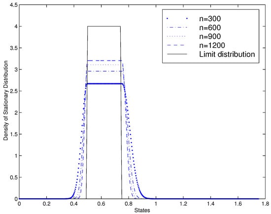
Figure 1. Convergence of the stationary distribution density for the repairman problem (with $\lambda =0.5$, $\mu =1$, $r_0=\lambda /\mu =0.5$ and $m_0=0.75$).

5. Concluding Remarks

We have presented the use of Gibbs distributions as a way to prove the convergence of the stationary distribution of the repairman problem in the averaging series scheme. The key contributions of this work are the weak convergence Gibbs distribution when the potential depends on a parameter $\theta$ and the transformation of the repairman stationary probabilities to Gibbs distributions. It will be of interest, on the one hand, to try to establish the same kind of results in a diffusion approximation scheme. Beyond the repairman problem, it would be of interest to apply this method to other similar problems. This problem must be rescaled in time when the finite state space becomes infinite. On the other hand, other work of interest can be performed in the direction of large deviations to provide a rate of convergence to the stationary distribution, see, e.g., [16].

References

- Billingsley, P. Convergence of Probability Measures; Wiley: Hoboken, NJ, USA, 1999. [Google Scholar]
- Dudley, R.M. Real Analysis and Probability; Wadsworth: Belmont, CA, USA, 1989. [Google Scholar]
- Ethier, S.N.; Kurtz, T.G. Markov Processes: Characterization and Convergence; Wiley: Hoboken, NJ, USA, 1986. [Google Scholar]
- Koroliuk, V.S.; Limnios, N. Stochastic Systems in Merging Phase Space; World Scientific: Singapore, 2005. [Google Scholar]
- Hwang, C.R. Laplace’s Method Revisited: Weak Convergence of Probability Measures. Ann. Probab. 1980, 6, 1177–1182. [Google Scholar] [CrossRef]
- Kaniovski, Y.; Pflug, G. Limit Thoerems for Stationary Distributions of Birth-and-Death Processes; Technical Report, IR–97–041; IIASA: Laxenburg, Austria, 1997. [Google Scholar]
- Iglehart, D.L. Limit approximations for the many servers queue and repairman problem. J. Appl. Probab. 1965, 2, 429–441. [Google Scholar] [CrossRef]
- Korolyuk, V.S. Maintenance Problems for Repairable Markov Systems. In Statistical and Probabilistics Models in Reliability; Ionescu, C., Limnios, N., Eds.; Birkhäuser: Boston, MA, USA, 1999. [Google Scholar]
- Crampes, C.; Renault, J. The repairman problem revisited. Ann. Econ. Stat. 2016, 7–24. [Google Scholar] [CrossRef]
- Jain, M.; Shekhar, C.; Shukla, S. Queueing analysis of machine repair problem with controlled rates and working vacation under F-policy. Proc. Natl. Acad. Sci. India Sect. Phys. Sci. 2016, 86, 21–31. [Google Scholar] [CrossRef]
- Chetouani, H.; Korolyuk, V.S. Stationary Distribution for Repairable Systems. Appl. Stoch. Models Bus. Ind. 2000, 16, 179–196. [Google Scholar] [CrossRef]
- Gihman, I.I.; Skorohod, A.V. Theory Stochastic Processes; Springer: Berlin/Heidelberg, Germany, 1974; Volume 1–3. [Google Scholar]
- Rogers, L.C.G.; Williams, D. Diffusions, Markov Processes, and Martingales; Volume 1: Foundations; Wiley: Chichester, UK, 1994. [Google Scholar]
- Khasminskii, R. Stability of the Solutions of Systems of Differential Equations under Random Disturbance of Their Parameters; Nauka: Moscow, Russia, 1969. [Google Scholar]
- Rudin, W. Functional Analysis; McGraw-Hill: New York, NY, USA, 1991. [Google Scholar]
- Dupuis, P.; Laschos, V.; Ramanan, K. Large deviations for configurations generated by Gibbs distributions with energy functionals consisting of singular interaction and weakly confining potentials. Electron. J. Probab. 2020, 25, 1–41. [Google Scholar] [CrossRef]
Disclaimer/Publisher’s Note: The statements, opinions and data contained in all publications are solely those of the individual author(s) and contributor(s) and not of MDPI and/or the editor(s). MDPI and/or the editor(s) disclaim responsibility for any injury to people or property resulting from any ideas, methods, instructions or products referred to in the content. |
© 2023 by the authors. Licensee MDPI, Basel, Switzerland. This article is an open access article distributed under the terms and conditions of the Creative Commons Attribution (CC BY) license (https://creativecommons.org/licenses/by/4.0/).