Two-Dimensional Scattering of Line Source Electromagnetic Waves by a Layered Obstacle

Abstract

We consider the scattering problem of line source electromagnetic waves using a multi-layered obstacle with a core, which may be a perfect conductor, a dielectric, or has an impedance surface. We formulate this problem in two dimensions and we prove some useful scattering relations. In particular, we state and prove a reciprocity principle and a general scattering theorem for line source waves for any possible positions of the source. These theorems can be used to approximate the far-field pattern in the low-frequency theory. Moreover, an optical theorem is recovered as a corollary of the general scattering theorem. Finally, we obtain a mixed reciprocity relation which can be used in proving the uniqueness results of the inverse scattering problems.

1. Introduction

This paper is concerned with relations for the time-harmonic electromagnetic scattering of a multi-layered scatterer. An obstacle of this type is made up of a nested body consisting of a finite number of homogeneous layers. On the surfaces of the layers the dielectric transmission conditions are imposed. The scatterer’s core may be a perfect conductor, a dielectric, or has an impedance surface. In the time-harmonic scattering theory [1] some theorems between the scattered fields of two problems which correspond to two distinct incident waves for the same scatterer appear. The incident waves can have a plane or line source. These properties are referred to as scattering theorems. In this work, we state and prove some scattering theorems and, in particular, a reciprocity, a general, a mixed reciprocity, and an optical theorem for a multi-layered scatterer which is excited by line source waves.

The reciprocity principle for line sources connects the total fields in two layers. The total field at $P_1$ due to a source at $P_2$ relates the total field at $P_2$ due to a source at $P_1$. A mixed reciprocity theorem associates the scattered field corresponding to a plane wave incident on a scatterer with the far-field pattern corresponding to a line source. The general theorem connects the far-field pattern generators (which are defined in [2] Formula (15)) at $P_1$ and $P_2$. The optical theorem for a plane incident field with direction of propagation $\widehat{\mathit{d}}$ states the total energy (the sum of the scattered and the absorption cross-section) that the obstacle removes for the incident field is proportional to the far-field pattern, which is valued in $\widehat{\mathit{d}}$. In case of line source waves, the far-field pattern is replaced by a far-field pattern generator. This theorem is obtained from the general theorem for $P_1=P_2$.

Using the reciprocity theorem, we can prove that the far-field operator corresponding to particular scattering problems is injective, with a dense range. These properties lead to a solution for the inverse scattering problems, Refs. [3,4,5]. The general scattering theorem is utilized in order to found the eigenvalues and eigenfunctions of the far-field operator and then to solve the inverse scattering problem using the linear sampling method or the factorization method [3,4,6]. The optical theorem can be used to evaluate the energy scattered by an obstacle, Refs. [1,7]. It is worth mentioning that these scattering relations can be mainly used in solving inverse scattering problems. In [8] near-field inverse scattering problems for ellipsoid scatterers have been solved.

A multi-layered scatterer for acoustic waves in three dimensions is described in [9]. Three-dimensional scattering relations have been proved for various kinds of scatterers. Indicatively, we refer to [1] for electromagnetic and [10] for elastic waves. Reciprocity, scattering, and optical theorems for acoustic and electromagnetic waves have been proven by Twersky in [11,12,13]. In view of these results, and by applying the low-frequency theory, he calculated an approximation of the real part of the far-field pattern. Reciprocity theorems for acoustic and electromagnetic waves are contained in the books [4,14] by Colton and Kress. In the book [1] written by Dassios and Kleinman, reciprocity, general, and optical theorems have also been recorded. In [15], Angell et al. have proven a reciprocity relation for electromagnetic scattering corresponding to a scatterer with an impedance boundary. Recently, a general optical theorem for an arbitrary multipole excitation is proven in [7] and scattering cross sections are evaluated in [16,17]. Corresponding theorems for elastic waves have been proven in [10] by using spherical coordinates.

Furthermore, in the case of three-dimensional multi-layered scatterers, scattering relations have been proven for acoustic waves in [9]. Scattering theorems for spherical waves have been proven in [2] (acoustic and electromagnetic). Moreover, in [2], a mixed reciprocity relation has been proven. In [18] Potthast has studied an inverse acoustic scattering problem using a mixed reciprocity relation for a piecewise constant inhomogeneous medium.

Following the procedure which is described by Colton and Cakoni in [3], the three dimensional electromagnetic scattering problem is reduced to a system of Helmholtz equations for a two-dimensional multi-layered scatterer. This kind of scatterer appears when a multi-layered infinitely long cylinder (all the layers have a common axis) is intersected vertically by a plane. Two-dimensional scattering theorems have been proven in [3,19]. In [20], plane electromagnetic scattering is studied, whereas in [21] line source elastic waves are studied. In [22], a mixed reciprocity principle is proven in two dimensions.

In the majority of the papers, the source which generates the incident wave is located in the exterior of the scatterer. In cases where the source is located in the interior of the scatterer, there are some important applications. Specifically, the detection of buried objects in a layered background medium requires the solution of an inverse scattering problem in which the source is located in an interior layer. Moreover, for the study of seismic waves, it is necessary to put the sources inside the layered media. In [23], inversion algorithms for determining the geometrical and physical characteristics of a spherical scatterer, which is excited by a line source, are developed. In [6] an inverse scattering problem for an object which is buried in a layered medium is studied. There are also applications in medicine, Ref. [24], such as implantation inside the human head for hyperthermia or biotelemetry purposes, Ref. [25], results (scattering theorems) are used for a scatterer, which is either a layered ellipsoid or sphere with internal sources.

First, in Section 2, we formulate two-dimensional scattering problems for a multi-layered scatterer for three different imposed boundary conditions on its core. In Section 3, we state and prove a two-dimensional reciprocity principle in the case of line source waves. Defining the line source generator, a general scattering theorem in classical form is proven in Section 4. In both Section 3 and Section 4, a multi-layered scatterer is excited by two line source waves located at any two layers. In Section 5, a mixed theorem is proven when the scatterer is excited by a line source and a plane wave. In Section 6, we formulate an optical theorem for the corresponding scattering problems.

2. Formulation

We consider electromagnetic scattering by a piecewise homogeneous obstacle $\tilde{D}$ in ${\mathbb{R}}^3$ with a $C^2$-boundary ${\tilde{S}}_0=\partial \tilde{D}$. The exterior ${\tilde{D}}_0={\mathbb{R}}^3\setminus \overline{\tilde{D}}$ of the obstacle is an infinite homogeneous isotropic medium with electric permittivity ${\epsilon }_0$, magnetic permeability ${\mu }_0$, and vanishing conductivity. The interior of $\tilde{D}$ is divided by means of closed and nonintersecting $C^2$-surfaces ${\tilde{S}}_j$, $j=1,2,\dots ,N-1$, $N\ge 2$ into layers ${\tilde{D}}_j$, $j=1,2,\dots ,N$, with $\partial {\tilde{D}}_{j-1}\cap \partial {\tilde{D}}_j={\tilde{S}}_{j-1}$. The surface ${\tilde{S}}_{j-1}$ surrounds ${\tilde{S}}_j$ and there is one normal unit vector $\widehat{\mathit{\nu }}\left(\mathit{x}\right)$ at each point $\mathit{x}$ of any surface ${\tilde{S}}_j$ pointing into ${\tilde{D}}_j$. 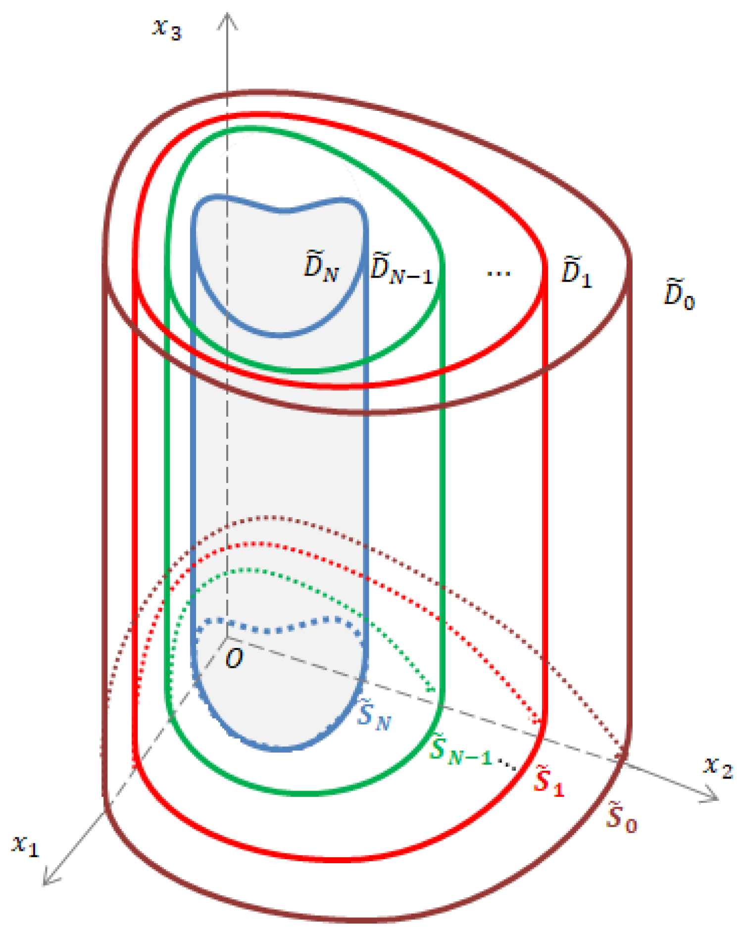The region ${\tilde{D}}_N$, within which lies the origin, is the core of the obstacle, which may be a dielectric, a perfect conductor, or an imperfect conductor. The layer ${\tilde{D}}_j$ is a homogeneous isotropic medium with electric permittivity ${\epsilon }_j$, magnetic permeability ${\mu }_j$, and vanishing conductivity. All the physical parameters ${\epsilon }_j$ and ${\mu }_j$ are positive constants. The geometry of the electromagnetic scattering problem in ${\mathbb{R}}^3$ is presented in Figure 1.

The total electric and magnetic fields ${\mathit{E}}_j$ and ${\mathit{H}}_j$ in ${\tilde{D}}_j$ satisfy the time-harmonic Maxwell equations [1],

$$\mathrm{curl}{\mathit{E}}_j=i\omega {\mu }_j{\mathit{H}}_j,\mathrm{curl}{\mathit{H}}_j=-i\omega {\epsilon }_j{\mathit{E}}_j\mathrm{in}{\tilde{D}}_j,j=0,1,\dots ,N,$$

(1)

where $\omega$ is the angular frequency.

The corresponding scattered electromagnetic field ${\mathit{E}}^{\mathrm{s}}$, ${\mathit{H}}^{\mathrm{s}}$ satisfies the Silver–Müller radiation condition

$${\displaystyle \underset{\left|\mathit{x}\right|⟶\infty }{lim}\left({\mathit{H}}^{\mathrm{s}}\times \mathit{x}-\left|\mathit{x}\right|{\mathit{E}}^{\mathrm{s}}\right)=\mathbf{0},}$$

(2)

uniformly in all directions $\widehat{\mathit{x}}={\displaystyle \frac{\mathit{x}}{\left|\mathit{x}\right|}}$. The total electromagnetic field ${\mathit{E}}_j$, ${\mathit{H}}_j$ in ${\tilde{D}}_j$ satisfies

$${\mathit{E}}_j={\mathit{E}}^{\mathrm{i}}+{\mathit{E}}^{\mathrm{s}},{\mathit{H}}_j={\mathit{H}}^{\mathrm{i}}+{\mathit{H}}^{\mathrm{s}}\in {\tilde{D}}_j,$$

(3)

where ${\mathit{E}}^{\mathrm{i}}$, ${\mathit{H}}^{\mathrm{i}}$ is the incident wave field. All the fields ${\mathit{E}}_j$, ${\mathit{H}}_j$, ${\mathit{E}}^{\mathrm{i}}$, ${\mathit{H}}^{\mathrm{i}}$, ${\mathit{E}}^{\mathrm{s}}$, ${\mathit{H}}^{\mathrm{s}}$ are divergence-free.

The transmission conditions on the surface ${\tilde{S}}_j$ for $j=0,1,\dots ,N-2$ are

$$\begin{array}{c}\hfill \widehat{\mathit{\nu }}\times {\mathit{E}}_j=\widehat{\mathit{\nu }}\times {\mathit{E}}_{j+1}\mathrm{on}{\tilde{S}}_j,\end{array}$$

(4)

$$\begin{array}{c}\hfill \widehat{\mathit{\nu }}\times {\mathit{H}}_j=\widehat{\mathit{\nu }}\times {\mathit{H}}_{j+1}\mathrm{on}{\tilde{S}}_j.\end{array}$$

(5)

On the surface ${\tilde{S}}_{N-1}$ of the core, we impose either the perfect conductor boundary condition

$$\widehat{\mathit{\nu }}\times {\mathit{E}}_{N-1}=\mathbf{0}\mathrm{on}{\tilde{S}}_{N-1},$$

(6)

or the dielectric transmission conditions

$$\begin{array}{c}\hfill \widehat{\mathit{\nu }}\times {\mathit{E}}_{N-1}=\widehat{\mathit{\nu }}\times {\mathit{E}}_N\mathrm{on}{\tilde{S}}_{N-1},\end{array}$$

(7)

$$\begin{array}{c}\hfill \widehat{\mathit{\nu }}\times {\mathit{H}}_{N-1}=\widehat{\mathit{\nu }}\times {\mathit{H}}_N\mathrm{on}{\tilde{S}}_{N-1},\end{array}$$

(8)

or the impedance boundary condition

$$\widehat{\mathit{\nu }}\times \mathrm{curl}{\mathit{E}}_{N-1}-i\lambda (\widehat{\mathit{\nu }}\times {\mathit{E}}_{N-1})\times \widehat{\mathit{\nu }}=\mathbf{0}\mathrm{on}{\tilde{S}}_{N-1},$$

(9)

where $\lambda >0$ is the surface impedance.

In the present work, we are interested in proving scattering relations that both play an important role in studying inverse scattering problems, see Ref. [3]. Specifically, the general scattering theorem is applied to the computation of the far-field pattern in the low-frequency theory (see [1]). The study of these relations will be done in two dimensions for the line source waves of the following scattering problems. The first problem, which corresponds to the perfect conductor core, is defined by Equations (1)–(6). The second one, which corresponds to the dielectric transmission condition of the core, is defined by Equations (1)–(5), (7) and (8). The third one, which corresponds to the impedance boundary condition of the core, is defined by Equations (1)–(5) and (9).

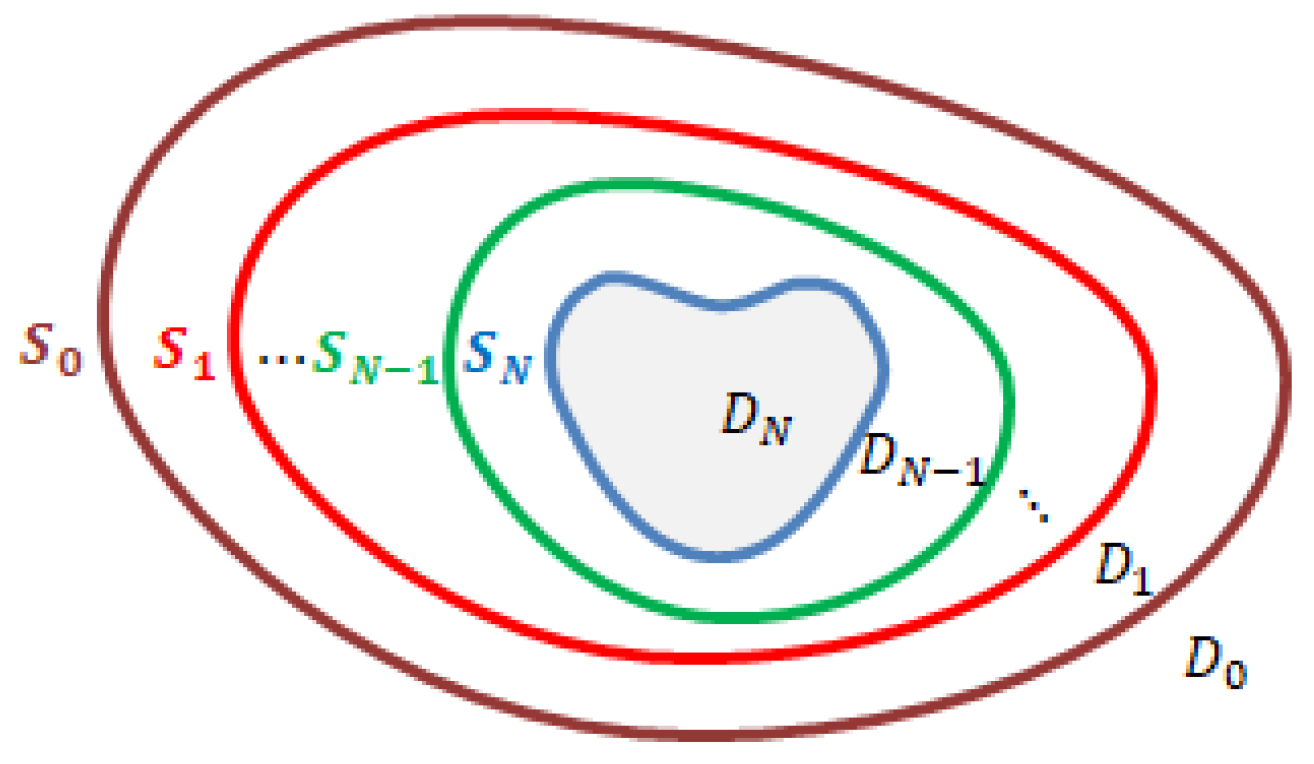
We suppose that $\tilde{D}=\left\{x=(x_1,x_2,x_3)\in {\mathbb{R}}^3:(x_1,x_2)\in D,x_3\in \mathbb{R}\right\}$ is an infinitely long cylinder which is oriented parallel to the $x_3$-axis. The cross-section D of $\tilde{D}$ in the $x_1{x}_2$-plane will be referred to as a two-dimensional scatterer. We also suppose that ${\tilde{S}}_j$, $j=1,\dots ,N-1$, are infinitely long cylindrical surfaces. The $x_1{x}_2$-plane intersects the surfaces ${\tilde{S}}_j$ at the $C^2$-curves $S_j$, see Figure 2.

Following the process specified by Cakoni and Colton in Ref. [3] (pp. 47 and 83), for the electric fields, we make the additional assumption that ${\mathit{E}}^{\mathrm{i}}=(0,0,{\mathcal{U}}^{\mathrm{i}}$, ${\mathit{E}}_j=(0,0,{\mathcal{U}}_j),$ where ${\mathcal{U}}_j$ is the total field in $D_j$. The incident field can be either a plane wave

$${\mathcal{U}}^{\mathrm{i}}(\mathit{x},\widehat{\mathit{d}})=e^{i{k}_0\mathit{x}·\widehat{\mathit{d}}},$$

(10)

where $k_0=\omega \sqrt{{\epsilon }_0{\mu }_0}$ is the wave number in $D_0$ and $\widehat{\mathit{d}}\in {\mathbb{R}}^2$ is the incident direction with $|\widehat{\mathit{d}}|=1$, [3], or a line source wave, [26],

$${\mathrm{\Phi }}^{\mathrm{i}}(\mathit{x},\mathit{z})={\displaystyle \frac{i}{4}}{H}_0^{\left(1\right)}(k_0|\mathit{x}-\mathit{z}|),$$

(11)

where $H_0^{\left(1\right)}$ is the zero order Hankel function of the first kind. Using these assumptions and applying the Maxwell Equation (1), we obtain ${\mathit{H}}^{\mathrm{i}}=(H_1^{\mathrm{i}},H_2^{\mathrm{i}},0)$, ${\mathit{H}}_j=(H_{j1},H_{j2},0)$, $j=0,1,\dots ,N$ and the following equations in $D_j$

$$\begin{array}{c}\hfill {\displaystyle \frac{\partial {\mathcal{U}}_j}{\partial x_2}}=i\omega {\mu }_j{H}_{j1},{\displaystyle \frac{\partial {\mathcal{U}}_j}{\partial x_1}}=-i\omega {\mu }_j{H}_{j2},\end{array}$$

(12)

$$\begin{array}{c}\hfill {\displaystyle \frac{\partial H_{j2}}{\partial x_1}}-{\displaystyle \frac{\partial H_{j1}}{\partial x_2}}=-i\omega {\epsilon }_j{\mathcal{U}}_j.\end{array}$$

(13)

Equations (12) and (13) imply that the $x_3$-component ${\mathcal{U}}_j$ of ${\mathit{E}}_j$ satisfies the Helmholtz equation

$$\mathrm{\Delta }{\mathcal{U}}_j+k_j^2{\mathcal{U}}_j=0\mathrm{in}{D}_j,$$

(14)

for $j=0,1,\dots ,N-1$ for the perfect conductor or the impedance boundary condition on the core core and $j=0,1,\dots ,N$ for the dielectric core. The symbol $\mathrm{\Delta }={\displaystyle \frac{{\partial }^2}{\partial x_1^2}}+{\displaystyle \frac{{\partial }^2}{\partial x_2^2}}$ stands for the two-dimensional Laplace operator. The $x_3$-component ${\mathcal{U}}_j$ of the total electric field ${\mathit{E}}_j$ in $D_j$ is given by

$${\mathcal{U}}_j\left(\mathit{x}\right)={\mathcal{U}}^{\mathrm{i}}\left(\mathit{x}\right)+{\mathcal{U}}^{\mathrm{s}}\left(\mathit{x}\right),\mathit{x}\in D_j,$$

(15)

where ${\mathcal{U}}^{\mathrm{s}}$ is the $x_3$-component of the scattered field ${\mathit{E}}^{\mathrm{s}}$. Specifically, ${\mathcal{U}}^{\mathrm{s}}\left(\mathit{x}\right)$, $\mathit{x}\in D_0$ satisfies the Sommerfeld radiation condition

$${\displaystyle \underset{\left|\mathit{x}\right|\to \infty }{lim}\sqrt{\left|\mathit{x}\right|}\left({\displaystyle \frac{\partial {\mathcal{U}}^{\mathrm{s}}}{\partial \mathit{\nu }}}-i{k}_0{\mathcal{U}}^{\mathrm{s}}\right)=0.}$$

(16)

The transmission condition Equations (4) and (5) are written in terms of the $x_3$-component ${\mathcal{U}}_j$ of the total electric field ${\mathit{E}}_j$, $j=0,1,\dots ,N-2$, as

$$\begin{array}{cc}\hfill {\mathcal{U}}_j& ={\mathcal{U}}_{j+1}\mathrm{on}{S}_j,\hfill \end{array}$$

(17)

$$\begin{array}{cc}\hfill {\displaystyle \frac{\partial {\mathcal{U}}_j}{\partial \mathit{\nu }}}& ={\displaystyle \frac{{\mu }_j}{{\mu }_{j+1}}}{\displaystyle \frac{\partial {\mathcal{U}}_{j+1}}{\partial \mathit{\nu }}}\mathrm{on}{S}_j.\hfill \end{array}$$

(18)

The boundary condition Equation (6) for the perfect conductor core is reformulated as

$${\mathcal{U}}_{N-1}=0\mathrm{on}{S}_{N-1}.$$

(19)

The transmission condition Equations (7) and (8) for the dielectric conductor are rewritten as

$$\begin{array}{cc}\hfill {\mathcal{U}}_{N-1}& ={\mathcal{U}}_N\mathrm{on}{S}_{N-1},\hfill \end{array}$$

(20)

$$\begin{array}{cc}\hfill {\displaystyle \frac{\partial {\mathcal{U}}_{N-1}}{\partial \mathit{\nu }}}& ={\displaystyle \frac{{\mu }_{N-1}}{{\mu }_N}}{\displaystyle \frac{\partial {\mathcal{U}}_N}{\partial \mathit{\nu }}}\mathrm{on}{S}_{N-1},\hfill \end{array}$$

(21)

and for the impedance boundary condition Equation (9), we have

$${\displaystyle \frac{\partial {\mathcal{U}}_{N-1}}{\partial \mathit{\nu }}}=-i\lambda {\mathcal{U}}_{N-1}\mathrm{on}{S}_{N-1}.$$

(22)

Summarizing the above analysis, we formulate the following three two-dimensional scattering problems. The first problem is defined by Equations (14)–(19) and is denoted by $\left(P_1\right)$, the second one is defined by Equations (14)–(18), (20) and (21) and is denoted by $\left(P_2\right)$, and the third one is defined by Equations (14)–(18) and (22) and is denoted by $\left(P_3\right)$. The well-posedness of these problems can be obtained by extending the techniques of [27].

In all the above problems, we assume that the multi-layered scatterer is excited by two line source waves located at any two layers. In case of the mixed reciprocity, the scatterer is excited by a line source and a plane wave.

We will denote by ${\mathcal{U}}^{\mathrm{s}}(\mathit{x},\widehat{\mathit{d}})$, ${\mathcal{U}}^{\infty }(\widehat{\mathit{x}},\widehat{\mathit{d}})$ and ${\mathcal{U}}_j(\mathit{x},\widehat{\mathit{d}})$ the dependence of the scattered field, the far-field pattern, and the total field in $D_j$ on the incident direction $\widehat{\mathit{d}}$. For incident line source wave at $\mathit{z}$, we utilize the fundamental solution

$${\mathrm{\Phi }}^{\mathrm{i}}(\mathit{x},\mathit{z})={\displaystyle \frac{i}{4}}{H}_0^{\left(1\right)}(k_0|\mathit{x}-\mathit{z}|),$$

(23)

where $H_0^{\left(1\right)}$ is the zero-order Hankel function of the first kind. We will denote by ${\mathrm{\Phi }}_j(\mathit{x},\mathit{z})$, ${\mathrm{\Phi }}^{\mathrm{s}}(\mathit{x},\mathit{z})$, and ${\mathrm{\Phi }}^{\infty }(\widehat{\mathit{x}},\mathit{z})$ to represent the dependence of the total field in $D_j$, $j=0,1,\dots ,N$, the scattered field, and the far-field pattern on the position of the source $\mathit{z}\in {\mathbb{R}}^2$.

The scattered line source field has the following asymptotic behaviour in two dimensions

$${\mathrm{\Phi }}^{\mathrm{s}}(\mathit{x},\mathit{z})={\displaystyle \frac{e^{i{k}_0\left|\mathit{x}\right|}}{\sqrt{\left|\mathit{x}\right|}}}{\mathrm{\Phi }}^{\infty }(\widehat{\mathit{x}},\mathit{z})+{\mathcal{O}\left(\right|\mathit{x}|}^{-3/2}),|\mathit{x}|\to \infty ,$$

(24)

uniformly in all directions $\widehat{\mathit{x}}={\displaystyle \frac{\mathit{x}}{\left|\mathit{x}\right|}}$ [3]. The far-field pattern ${\mathrm{\Phi }}^{\infty }(\widehat{\mathit{x}},\mathit{z})$ is given by [3],

$${\mathrm{\Phi }}^{\infty }(\widehat{\mathit{x}},\mathit{z})={\displaystyle \frac{e^{i\pi /4}}{\sqrt{8\pi k_0}}}{\int }_{S_0}\left[{\mathrm{\Phi }}^{\mathrm{s}}(\mathbf{y},\mathit{z}){\displaystyle \frac{\partial }{\partial \mathit{\nu }\left(\mathbf{y}\right)}}{e}^{-i{k}_0\widehat{\mathit{x}}·\mathbf{y}}-{\displaystyle \frac{\partial {\mathrm{\Phi }}^s(\mathbf{y},\mathit{z})}{\partial \mathit{\nu }\left(\mathbf{y}\right)}}{e}^{-i{k}_0\widehat{\mathit{x}}·\mathbf{y}}\right]ds\left(\mathbf{y}\right).$$

(25)

In the rest of the paper, we will use Twersky’s notation [11],

$${\left\{u,v\right\}}_S={\int }_S\left(u{\displaystyle \frac{\partial v}{\partial \mathit{\nu }}}-v{\displaystyle \frac{\partial u}{\partial \mathit{\nu }}}\right)ds.$$

(26)

As we can see, the far-field pattern is expressed through the Twersky’s notation as

$${\mathrm{\Phi }}^{\infty }(\widehat{\mathit{x}},\mathit{z})={\displaystyle \frac{e^{i\pi /4}}{\sqrt{8\pi k_0}}}{\left\{{\mathrm{\Phi }}^{\mathrm{s}}(·,\mathit{z}),{\mathcal{U}}^{\mathrm{i}}(·,-\widehat{\mathit{x}})\right\}}_{S_0}.$$

(27)

3. Reciprocity for Line Source Waves

For incident plane waves, similar scattering relations have already been proven in [9] for three dimensions and in [19] for two dimensions. Now, we will emphasize proving the corresponding relations for line source waves in two dimensions. For this purpose, we consider two line source waves at ${\mathit{z}}_{\sigma }\in D_{\sigma }$ and ${\zeta }_{\tau }\in D_{\tau }$, with $0\le \sigma \le \tau \le N$. Then, we prove the following lemma.

Lemma 1.

Let ${\mathrm{\Phi }}^{\mathrm{i}}(\mathit{x},{\mathit{z}}_{\sigma })$ be an incident line source wave at ${\mathit{z}}_{\sigma }$. Let ${\mathrm{\Phi }}^{\mathrm{i}}(\mathit{x},{\zeta }_{\tau })$ be an incident line source wave at ${\zeta }_{\tau }$ with corresponding scattered field ${\mathrm{\Phi }}^{\mathrm{s}}(\mathit{x},{\zeta }_{\tau })$ and total field ${\mathrm{\Phi }}_{\tau }(\mathit{x},{\zeta }_{\tau })$ in $D_{\tau }$. Then, it holds

$$\begin{array}{ccc}\hfill \underset{R\to \infty }{lim}{\{{\mathrm{\Phi }}^{\mathrm{i}}(\mathit{x},{\mathit{z}}_{\sigma }),{\mathrm{\Phi }}^{\mathrm{s}}(\mathit{x},{\zeta }_{\tau })\}}_{S_{O,R}}& =& 0,\hfill \end{array}$$

(28)

$$\begin{array}{ccc}\hfill \underset{{ϵ}_{\sigma }\to 0}{lim}{\{{\mathrm{\Phi }}^{\mathrm{i}}(\mathit{x},{\mathit{z}}_{\sigma }),{\mathrm{\Phi }}^{\mathrm{s}}(\mathit{x},{\zeta }_{\tau })\}}_{S_{{\mathit{z}}_{\sigma },{ϵ}_{\sigma }}}& =& {\mathrm{\Phi }}^{\mathrm{s}}({\mathit{z}}_{\sigma },{\zeta }_{\tau }),\hfill \end{array}$$

(29)

$$\begin{array}{ccc}\hfill \underset{{ϵ}_{\tau }\to 0}{lim}{\{{\mathrm{\Phi }}_{\tau }(\mathit{x},{\mathit{z}}_{\sigma }),{\mathrm{\Phi }}_{\tau }(\mathit{x},{\zeta }_{\tau })\}}_{S_{{\zeta }_{\tau },{ϵ}_{\tau }}}& =& -{\mathrm{\Phi }}_{\tau }({\zeta }_{\tau },{\mathit{z}}_{\sigma }),\hfill \end{array}$$

(30)

where $S_{{\mathit{z}}_{\sigma },{ϵ}_{\sigma }}$ is a disc centered at ${\mathit{z}}_{\sigma }$ with radius ${ϵ}_{\sigma }$, $S_{{\zeta }_{\tau },{ϵ}_{\tau }}$ is a disc centered at ${\zeta }_{\tau }$ with radius ${ϵ}_{\tau }$, and $S_{O,R}$ is a disc centered at the origin with radius R surrounding the points ${\mathit{z}}_{\sigma }$ and ${\zeta }_{\tau }$.

Proof. 

Since ${\mathrm{\Phi }}^{\mathrm{i}}(\mathit{x},{\mathit{z}}_{\sigma })$ and ${\mathrm{\Phi }}^{\mathrm{s}}(\mathit{x},{\zeta }_{\tau })$ are solutions of the Helmholtz equation for $\mathit{x}\ne {\mathit{z}}_{\sigma }$ and satisfy the Sommerfeld radiation condition, we obtain relation Equation (28).

Using the asymptotic forms, Ref. [3],

$$\begin{array}{ccc}\hfill {\mathrm{\Phi }}^{\mathrm{i}}(\mathit{x},{\mathit{z}}_{\sigma })& =& {\displaystyle \frac{1}{2\pi }}log{\displaystyle \frac{1}{|\mathit{x}-{\mathit{z}}_{\sigma }|}}+\mathcal{O}\left(1\right),\hfill \end{array}$$

(31)

$$\begin{array}{ccc}\hfill {\displaystyle \frac{\partial }{\partial \mathit{\nu }\left(\mathit{x}\right)}}{\mathrm{\Phi }}^{\mathrm{i}}(\mathit{x},{\mathit{z}}_{\sigma })& =& -{\displaystyle \frac{1}{2\pi }}{\displaystyle \frac{1}{|\mathit{x}-{\mathit{z}}_{\sigma }|}}+\mathcal{O}\left(|\mathit{x}-{\mathit{z}}_{\sigma }|log|\mathit{x}-{\mathit{z}}_{\sigma }|\right),\hfill \end{array}$$

(32)

as $|\mathit{x}-{\mathit{z}}_{\sigma }|\to 0$, applying the mean value theorem and letting $|\mathit{x}-{\mathit{z}}_{\sigma }|\to 0$ we obtain relation Equation (29).

For relation Equation (30), we replace ${\mathrm{\Phi }}_{\tau }(\mathit{x},{\zeta }_{\tau })={\mathrm{\Phi }}^{\mathrm{i}}(\mathit{x},{\zeta }_{\tau })+{\mathrm{\Phi }}^{\mathrm{s}}(\mathit{x},{\zeta }_{\tau })$ and we take

$${\{{\mathrm{\Phi }}_{\tau }(·,{\mathit{z}}_{\sigma }),{\mathrm{\Phi }}_{\tau }(·,{\zeta }_{\tau })\}}_{S_{{\zeta }_{\tau },{ϵ}_{\tau }}}={\{{\mathrm{\Phi }}_{\tau }(·,{\mathit{z}}_{\sigma }),{\mathrm{\Phi }}^{\mathrm{i}}(·,{\zeta }_{\tau })\}}_{S_{{\zeta }_{\tau },{ϵ}_{\tau }}}+{\{{\mathrm{\Phi }}_{\tau }(·,{\mathit{z}}_{\sigma }),{\mathrm{\Phi }}^{\mathrm{s}}(·,{\zeta }_{\tau })\}}_{S_{{\zeta }_{\tau },{ϵ}_{\tau }}}.$$

(33)

The first integral of the right-hand side of Equation (33) is equal to $-{\mathrm{\Phi }}_{\tau }({\zeta }_{\tau },{\mathit{z}}_{\sigma })$, due to relation Equation (29). For the last integral, taking into account the interior elliptic regularity, see Refs. [5,22,28], we have

$${\int }_{D_{{\zeta }_{\tau },{ϵ}_{\tau }}}\left[|{\mathrm{\Phi }}^{\mathrm{s}}(\mathit{x},{\zeta }_{\tau })|+|\nabla {\mathrm{\Phi }}^{\mathrm{s}}(\mathit{x},{\zeta }_{\tau })|\right]ds\left(\mathit{x}\right)\to 0,\mathrm{as}{ϵ}_{\tau }\to 0,$$

(34)

and by using the Cauchy–Schwarz inequality we conclude that

$${\{{\mathrm{\Phi }}_{\tau }(·,{\mathit{z}}_0),{\mathrm{\Phi }}^{\mathrm{s}}(·,{\zeta }_{\tau })\}}_{S_{{\zeta }_{\tau },{ϵ}_{\tau }}}=0.$$

(35)

□

Remark 1.

Relation Equation (29) is also valid if ${\mathrm{\Phi }}^{\mathrm{s}}(\mathit{x},{\zeta }_{\tau })$ is replaced by ${\mathrm{\Phi }}^{\mathrm{i}}(\mathit{x},{\zeta }_{\tau })$. In general, ${\mathrm{\Phi }}^{\mathrm{s}}(\mathit{x},{\zeta }_{\tau })$ can be replaced by bounded fields.

Next, we prove the following reciprocity theorem for line source waves and multi-layered scatterers in two dimensions.

Theorem 1.

Let ${\mathrm{\Phi }}^{\mathrm{i}}(·,{\mathit{z}}_{\sigma })$ and ${\mathrm{\Phi }}^{\mathrm{i}}(·,{\zeta }_{\tau })$ be two incident line source waves at ${\mathit{z}}_{\sigma }\in D_{\sigma }$ and ${\zeta }_{\tau }\in D_{\tau }$, respectively. Then the corresponding total fields ${\mathrm{\Phi }}_{\sigma }({\mathit{z}}_{\sigma },{\zeta }_{\tau })$ and ${\mathrm{\Phi }}_{\tau }({\zeta }_{\tau },{\mathit{z}}_{\sigma })$ for the scattering problem $\left(P_n\right)$, $n=1,2,3$, satisfy the reciprocity relation

$${\mu }_{\tau }{\mathrm{\Phi }}_{\sigma }({\mathit{z}}_{\sigma },{\zeta }_{\tau })={\mu }_{\sigma }{\mathrm{\Phi }}_{\tau }({\zeta }_{\tau },{\mathit{z}}_{\sigma }).$$

(36)

Proof. 

Due to the bilinearity of Equation (26), and taking into account tion ${\mathrm{\Phi }}_0={\mathrm{\Phi }}^{\mathrm{i}}+{\mathrm{\Phi }}^{\mathrm{s}}$, we have

$$\begin{array}{c}\hfill {\{{\mathrm{\Phi }}_0(·,{\mathit{z}}_{\sigma }),{\mathrm{\Phi }}_0(·,{\zeta }_{\tau })\}}_{S_0}={\left\{{\mathrm{\Phi }}^{\mathrm{i}}(·,{\mathit{z}}_{\sigma }),{\mathrm{\Phi }}^{\mathrm{i}}(·,{\zeta }_{\tau })\right\}}_{S_0}+{\left\{{\mathrm{\Phi }}^{\mathrm{i}}(·,{\mathit{z}}_{\sigma }),{\mathrm{\Phi }}^{\mathrm{s}}(·,{\zeta }_{\tau })\right\}}_{S_0}\\ \hfill +{\left\{{\mathrm{\Phi }}^{\mathrm{s}}(·,{\mathit{z}}_{\sigma }),{\mathrm{\Phi }}^{\mathrm{i}}(·,{\zeta }_{\tau })\right\}}_{S_0}+{\left\{{\mathrm{\Phi }}^{\mathrm{s}}(·,{\mathit{z}}_{\sigma }),{\mathrm{\Phi }}^{\mathrm{s}}(·,{\zeta }_{\tau })\right\}}_{S_0}.\end{array}$$

(37)

We initially consider the case $\sigma =\tau =0$, i.e., the two sources are outside of the scatterer. For the first integral of the right-hand side of relation Equation (37), since ${\mathrm{\Phi }}^{\mathrm{i}}(\mathit{x},{\mathit{z}}_0)$ and ${\mathrm{\Phi }}^{\mathrm{i}}(\mathit{x},{\zeta }_0)$ are regular solutions of the Helmholtz equation in $D_0\setminus \{{\mathit{z}}_0,{\zeta }_0\}$, an application of the scalar Green’s second theorem gives

$${\left\{{\mathrm{\Phi }}^{\mathrm{i}}(·,{\mathit{z}}_0),{\mathrm{\Phi }}^{\mathrm{i}}(·,{\zeta }_0)\right\}}_{S_0}=0.$$

(38)

For the computation of the next integral, we consider two small disjoint discs $S_{{\mathit{z}}_0,{ϵ}_0}$ and $S_{{\zeta }_0,{ϵ}_0^{\prime }}$ centered at ${\mathit{z}}_0$ and ${\zeta }_0$ with radius ${ϵ}_0$ and ${ϵ}_0^{\prime }$, respectively. We also consider a large disc $S_{O,R}$ centered at the origin with radius R surrounding the points ${\mathit{z}}_0$, ${\zeta }_0$ and the scatterer.

Since ${\mathrm{\Phi }}^{\mathrm{i}}(\mathit{x},{\mathit{z}}_0)$ and ${\mathrm{\Phi }}^{\mathrm{s}}(\mathit{x},{\zeta }_0)$ are solutions of the Helmholtz equation for $\mathit{x}\ne {\mathit{z}}_0,{\zeta }_0$, we apply the scalar Green’s second theorem and obtain

$$\begin{array}{ccc}\hfill {\left\{{\mathrm{\Phi }}^{\mathrm{i}}(·,{\mathit{z}}_0),{\mathrm{\Phi }}^{\mathrm{s}}(·,{\zeta }_0)\right\}}_{S_0}& =& {\left\{{\mathrm{\Phi }}^{\mathrm{i}}(·,{\mathit{z}}_0),{\mathrm{\Phi }}^{\mathrm{s}}(·,{\zeta }_0)\right\}}_{S_{O,R}}-{\left\{{\mathrm{\Phi }}^{\mathrm{i}}(·,{\mathit{z}}_0),{\mathrm{\Phi }}^{\mathrm{s}}(·,{\zeta }_0)\right\}}_{S_{{\mathit{z}}_0,{ϵ}_0}}\hfill \\ \hfill & & -{\left\{{\mathrm{\Phi }}^{\mathrm{i}}(·,{\mathit{z}}_0),{\mathrm{\Phi }}^{\mathrm{s}}(·,{\zeta }_0)\right\}}_{S_{{\zeta }_0,{ϵ}_0^{\prime }}}.\hfill \end{array}$$

(39)

Letting $R\to \infty$, ${ϵ}_0\to 0$, using Lemma 1, and taking into account that the last integral of Equation (39) is zero, due to the application of the scalar Green’s second theorem in $S_{{\zeta }_0,{ϵ}_0^{\prime }}$ and since ${\mathrm{\Phi }}^{\mathrm{i}}(\mathit{x},{\mathit{z}}_0)$ and ${\mathrm{\Phi }}^{\mathrm{s}}(\mathit{x},{\zeta }_0)$ are regular solutions of the Helmholtz equations for $\mathit{x}\ne {\mathit{z}}_0$, we obtain

$$\begin{array}{c}\hfill {\left\{{\mathrm{\Phi }}^{\mathrm{i}}(·,{\mathit{z}}_0),{\mathrm{\Phi }}^{\mathrm{s}}(·,{\zeta }_0)\right\}}_{S_0}=-{\mathrm{\Phi }}^{\mathrm{s}}({\mathit{z}}_0,{\zeta }_0).\end{array}$$

(40)

Similarly, we obtain

$$\begin{array}{c}\hfill {\left\{{\mathrm{\Phi }}^{\mathrm{s}}(·,{\mathit{z}}_0),{\mathrm{\Phi }}^{\mathrm{i}}(·,{\zeta }_0)\right\}}_{S_0}={\mathrm{\Phi }}^{\mathrm{s}}({\zeta }_0,{\mathit{z}}_0).\end{array}$$

(41)

Since ${\mathrm{\Phi }}^{\mathrm{s}}(·,{\mathit{z}}_0)$, ${\mathrm{\Phi }}^{\mathrm{s}}(·,{\zeta }_0)$ are radiating solutions of the Helmholtz equation in $D_0$, we have

$${\left\{{\mathrm{\Phi }}^{\mathrm{s}}(·,{\mathit{z}}_0),{\mathrm{\Phi }}^{\mathrm{s}}(·,{\zeta }_0)\right\}}_{S_0}=0.$$

(42)

The total fields ${\mathrm{\Phi }}_j(·,{\mathit{z}}_0)$ and ${\mathrm{\Phi }}_j(·,{\zeta }_0)$, $j=1,2,\dots ,N-1$, are regular solutions of the Helmholtz equation in $D_j$. Thus, the successive application of the scalar Green’s second theorem and the use of the transmission conditions on $S_j$ imply that

$${\{{\mathrm{\Phi }}_0(·,{\mathit{z}}_0),{\mathrm{\Phi }}_0(·,{\zeta }_0)\}}_{S_0}={\displaystyle \frac{{\mu }_0}{{\mu }_{N-1}}}{\{{\mathrm{\Phi }}_{N-1}(·,{\mathit{z}}_0),{\mathrm{\Phi }}_{N-1}(·,{\zeta }_0)\}}_{S_{N-1}}.$$

(43)

By using the imposed boundary conditions on $S_{N-1}$ for $\left(P_1\right)$ and $\left(P_3\right)$, we directly obtain that the integral is equal to zero. For $\left(P_2\right)$, we apply the transmission conditions, we use the scalar Green’s second theorem, and we obtain

$${\{{\mathrm{\Phi }}_0(·,{\mathit{z}}_0),{\mathrm{\Phi }}_0(·,{\zeta }_0)\}}_{S_0}=0.$$

(44)

Substituting relations Equations (38), (40)–(42) and (44) in Equation (37), we derive

$${\mathrm{\Phi }}^{\mathrm{s}}({\mathit{z}}_0,{\zeta }_0)={\mathrm{\Phi }}^{\mathrm{s}}({\zeta }_0,{\mathit{z}}_0).$$

(45)

From definition Equation (23) of the line source, we see that ${\mathrm{\Phi }}^{\mathrm{i}}({\mathit{z}}_0,{\zeta }_0)={\mathrm{\Phi }}^{\mathrm{i}}({\zeta }_0,{\mathit{z}}_0)$, and due to relation Equation (45), we have

$${\mathrm{\Phi }}_0({\mathit{z}}_0,{\zeta }_0)={\mathrm{\Phi }}_0({\zeta }_0,{\mathit{z}}_0).$$

(46)

Next, we consider the case $0=\sigma <\tau \le N$, i.e., one source is inside and the other one is outside the scatterer.

Taking into account that ${\mathrm{\Phi }}^{\mathrm{i}}(\mathit{x},{\mathit{z}}_0)$, ${\mathrm{\Phi }}^{\mathrm{i}}(\mathit{x},{\zeta }_{\tau })$ are solutions of the Helmholtz equation in D for $\mathit{x}\ne {\zeta }_{\tau }$ and by using Lemma 1, we obtain

$${\left\{{\mathrm{\Phi }}^{\mathrm{i}}(·,{\mathit{z}}_0),{\mathrm{\Phi }}^{\mathrm{i}}(·,{\zeta }_{\tau })\right\}}_{S_0}={\left\{{\mathrm{\Phi }}^{\mathrm{i}}(·,{\mathit{z}}_0),{\mathrm{\Phi }}^{\mathrm{i}}(·,{\zeta }_{\tau })\right\}}_{S_{{\zeta }_{\tau },{ϵ}_{\tau }}}=-{\mathrm{\Phi }}^{\mathrm{i}}({\zeta }_{\tau },{\mathit{z}}_0).$$

(47)

For the next integral of Equation (37), working as in the previous case, we obtain

$${\left\{{\mathrm{\Phi }}^{\mathrm{i}}(·,{\mathit{z}}_0),{\mathrm{\Phi }}^{\mathrm{s}}(·,{\zeta }_{\tau })\right\}}_{S_0}={\left\{{\mathrm{\Phi }}^{\mathrm{i}}(·,{\mathit{z}}_0),{\mathrm{\Phi }}^{\mathrm{s}}(·,{\zeta }_{\tau })\right\}}_{S_{O,R}}-{\left\{{\mathrm{\Phi }}^{\mathrm{i}}(·,{\mathit{z}}_0),{\mathrm{\Phi }}^{\mathrm{s}}(·,{\zeta }_{\tau })\right\}}_{S_{z_0,{ϵ}_0}}=-{\mathrm{\Phi }}^{\mathrm{s}}({\mathit{z}}_0,{\zeta }_{\tau }).$$

(48)

Moreover, it holds

$$\begin{array}{c}\hfill {\left\{{\mathrm{\Phi }}^{\mathrm{s}}(·,{\mathit{z}}_0),{\mathrm{\Phi }}^{\mathrm{i}}(·,{\zeta }_{\tau })\right\}}_{S_0}={\left\{{\mathrm{\Phi }}^{\mathrm{s}}(·,{\mathit{z}}_0),{\mathrm{\Phi }}^{\mathrm{s}}(·,{\zeta }_{\tau })\right\}}_{S_0}=0,\end{array}$$

(49)

since the involved functions are radiating solutions of the Helmholtz equation in $D_0$. For the total fields we have

$${\{{\mathrm{\Phi }}_0(·,{\mathit{z}}_0),{\mathrm{\Phi }}_0(·,{\zeta }_{\tau })\}}_{S_0}={\displaystyle \frac{{\mu }_0}{{\mu }_{N-1}}}{\{{\mathrm{\Phi }}_{N-1}(·,{\mathit{z}}_0),{\mathrm{\Phi }}_{N-1}(·,{\zeta }_{\tau })\}}_{S_{N-1}}+{\displaystyle \frac{{\mu }_0}{{\mu }_{\tau }}}{\{{\mathrm{\Phi }}_{\tau }(·,{\mathit{z}}_0),{\mathrm{\Phi }}_{\tau }(·,{\zeta }_{\tau })\}}_{S_{{\zeta }_{\tau },{ϵ}_{\tau }}}.$$

(50)

The first integral of the right-hand side is equal to zero due to the imposed boundary and transmission conditions on the surface $S_{N-1}$ of the core. Applying Lemma 1, we obtain

$${\{{\mathrm{\Phi }}_0(·,{\mathit{z}}_0),{\mathrm{\Phi }}_0(·,{\zeta }_{\tau })\}}_{S_0}=-{\displaystyle \frac{{\mu }_0}{{\mu }_{\tau }}}{\mathrm{\Phi }}_{\tau }({\zeta }_{\tau },{\mathit{z}}_0).$$

(51)

Substituting relation Equations (47)–(49) and (51) in Equation (37), we obtain

$${\mu }_0{\mathrm{\Phi }}_{\tau }({\mathit{z}}_0,{\zeta }_{\tau })={\mu }_{\tau }{\mathrm{\Phi }}_0({\zeta }_{\tau },{\mathit{z}}_0).$$

(52)

We finally consider the case $0<\sigma \le \tau \le N$, i.e., both of the sources are inside the scatterer.

It holds

$${\left\{{\mathrm{\Phi }}^{\mathrm{i}}(·,{\mathit{z}}_{\sigma }),{\mathrm{\Phi }}^{\mathrm{i}}(·,{\zeta }_{\tau })\right\}}_{S_0}=0,$$

(53)

since ${\mathrm{\Phi }}^{\mathrm{i}}(·,{\mathit{z}}_{\sigma })$ and ${\mathrm{\Phi }}^{\mathrm{i}}(·,{\zeta }_{\tau })$ are radiating solutions of the Helmholtz equation. Moreover, ${\mathrm{\Phi }}^{\mathrm{s}}(·,{\mathit{z}}_{\sigma })$ and ${\mathrm{\Phi }}^{\mathrm{s}}(·,{\zeta }_{\tau })$ are radiating solutions of the Helmholtz equation, and thus we obtain

$${\left\{{\mathrm{\Phi }}^{\mathrm{i}}(·,{\mathit{z}}_{\sigma }),{\mathrm{\Phi }}^{\mathrm{s}}(·,{\zeta }_{\tau })\right\}}_{S_0}={\left\{{\mathrm{\Phi }}^{\mathrm{s}}(·,{\mathit{z}}_{\sigma }),{\mathrm{\Phi }}^{\mathrm{i}}(·,{\zeta }_{\tau })\right\}}_{S_0}={\left\{{\mathrm{\Phi }}^{\mathrm{s}}(·,{\mathit{z}}_{\sigma }),{\mathrm{\Phi }}^{\mathrm{s}}(·,{\zeta }_{\tau })\right\}}_{S_0}=0.$$

(54)

Concerning the total fields, by successively applying the scalar Green’s second theorem, we have

$$\begin{array}{c}\hfill {\left\{{\mathrm{\Phi }}_0(·,{\mathit{z}}_{\sigma }),{\mathrm{\Phi }}_0(·,{\zeta }_{\tau })\right\}}_{S_0}={\displaystyle \frac{{\mu }_0}{{\mu }_{N-1}}}{\left\{{\mathrm{\Phi }}_{N-1}(·,{\mathit{z}}_{\sigma }),{\mathrm{\Phi }}_{N-1}(·,{\zeta }_{\tau })\right\}}_{S_{N-1}}\\ \hfill -{\displaystyle \frac{{\mu }_0}{{\mu }_{\sigma }}}{\left\{{\mathrm{\Phi }}_{\sigma }(·,{\mathit{z}}_{\sigma }),{\mathrm{\Phi }}_{\sigma }(·,{\zeta }_{\tau })\right\}}_{S_{z_{\sigma },{ϵ}_{\sigma }}}-{\displaystyle \frac{{\mu }_0}{{\mu }_{\tau }}}{\left\{{\mathrm{\Phi }}_{\tau }(·,{\mathit{z}}_{\sigma }),{\mathrm{\Phi }}_{\tau }(·,{\zeta }_{\tau })\right\}}_{S_{{\zeta }_{\tau },{ϵ}_{\tau }}}.\end{array}$$

(55)

Due to the boundary and the transmission conditions on the core and via Lemma 1, we obtain

$${\left\{{\mathrm{\Phi }}_0(·,{\mathit{z}}_{\sigma }),{\mathrm{\Phi }}_0(·,{\zeta }_{\tau })\right\}}_{S_0}=-{\displaystyle \frac{{\mu }_0}{{\mu }_{\sigma }}}{\mathrm{\Phi }}_{\sigma }({\mathit{z}}_{\sigma },{\zeta }_{\tau })+{\displaystyle \frac{{\mu }_0}{{\mu }_{\tau }}}{\mathrm{\Phi }}_{\tau }({\zeta }_{\tau },{\mathit{z}}_{\sigma }).$$

(56)

The substitution of relation Equations (53), (54) and (56) in Equation (37) implies the generation of relation Equation (36). □

Remark 2.

If the positions of the line source waves are located at the same layer or both of them are outside the scatterer, i.e., $\sigma =\tau$, then the reciprocity relation Equation (36) is reformulated as

$${\mathrm{\Phi }}_{\sigma }({\mathit{z}}_{\sigma },{\zeta }_{\sigma })={\mathrm{\Phi }}_{\sigma }({\zeta }_{\sigma },{\mathit{z}}_{\sigma }).$$

(57)

4. A General Scattering Theorem

As in the reciprocity theorem, we suppose that the scatterer D is excited by two line source waves. In what follows, $\overline{w}$ denotes the complex conjugate of w and $S^1$ denotes the unit disc in ${\mathbb{R}}^2$.

Lemma 2.

Let ${\mathrm{\Phi }}^{\mathrm{i}}(\mathit{x},{\mathit{z}}_{\sigma })$ be an incident line source wave at ${\mathit{z}}_{\sigma }$. For an incident line source wave ${\mathrm{\Phi }}^{\mathrm{i}}(\mathit{x},{\zeta }_{\tau })$ at ${\zeta }_{\tau }$ with corresponding scattered field ${\mathrm{\Phi }}^{\mathrm{s}}(\mathit{x},{\zeta }_{\tau })$ and far-field pattern ${\mathrm{\Phi }}^{\infty }(\widehat{\mathit{x}},{\zeta }_{\tau })$, we have

$$\begin{array}{ccc}\hfill \underset{R\to \infty }{lim}{\{\overline{{\mathrm{\Phi }}^{\mathrm{i}}(\mathit{x},{\mathit{z}}_{\sigma })},{\mathrm{\Phi }}^{\mathrm{s}}(\mathit{x},{\zeta }_{\tau })\}}_{S_{O,R}}& =& {\displaystyle \frac{2k_0{e}^{i\pi /4}}{\sqrt{8k_0\pi }}}{\int }_{S^1}{\mathrm{\Phi }}^{\infty }(\widehat{\mathit{x}},{\zeta }_{\tau })e^{i{k}_0\widehat{\mathit{x}}·{\mathit{z}}_{\sigma }}ds\left(\widehat{\mathit{x}}\right),\hfill \end{array}$$

(58)

$$\begin{array}{ccc}\hfill \underset{{ϵ}_{\sigma }\to 0}{lim}{\{\overline{{\mathrm{\Phi }}^{\mathrm{i}}(\mathit{x},{\mathit{z}}_{\sigma })},{\mathrm{\Phi }}^{\mathrm{s}}(\mathit{x},{\zeta }_{\tau })\}}_{S_{{\mathit{z}}_{\sigma },{ϵ}_{\sigma }}}& =& {\mathrm{\Phi }}^{\mathrm{s}}({\mathit{z}}_{\sigma },{\zeta }_{\tau }),\hfill \end{array}$$

(59)

$$\begin{array}{ccc}\hfill \underset{{ϵ}_{\tau }\to 0}{lim}{\{\overline{{\mathrm{\Phi }}_{\tau }(·,{\mathit{z}}_{\sigma })},{\mathrm{\Phi }}_{\tau }(·,{\zeta }_{\tau })\}}_{S_{{\zeta }_{\tau },{ϵ}_{\tau }}}& =& -\overline{{\mathrm{\Phi }}_{\tau }({\zeta }_{\tau },{\mathit{z}}_{\sigma })},\hfill \end{array}$$

(60)

where $S_{{\mathit{z}}_{\sigma },{ϵ}_{\sigma }}$ is a disc centered at ${\mathit{z}}_{\sigma }$ with radius ${ϵ}_{\sigma }$, $S_{{\zeta }_{\tau },{ϵ}_{\tau }}$ is a disc centered at ${\zeta }_{\tau }$ with radius ${ϵ}_{\tau }$ and $S_{O,R}$ is a disc centered at the origin with radius R surrounding the points ${\mathit{z}}_{\sigma }$ and ${\zeta }_{\tau }$.

Proof. 

Using the asymptotic form of the Hankel function $H_0^{\left(1\right)}(k_0\left|\mathit{y}\right|)$, see Refs. [3,29],

$$H_0^{\left(1\right)}(k_0\left|\mathit{y}\right|)=\sqrt{{\displaystyle \frac{2}{k_0\pi \left|\mathit{y}\right|}}}{e}^{i\left(k_0\right|\mathit{y}|-\frac{\pi }{4})}+{\mathcal{O}\left(\right|\mathit{y}|}^{-3/2}),|\mathit{y}|\to \infty ,$$

(61)

and the asymptotic relations [1]

$$\begin{array}{c}\hfill |\mathit{x}-{\mathit{z}}_{\sigma }|=|\mathit{x}|-\widehat{\mathit{x}}·{\mathit{z}}_{\sigma }+{\mathcal{O}\left(\right|\mathit{x}|}^{-1}),|\mathit{x}|\to \infty ,\end{array}$$

(62)

$$\begin{array}{c}\hfill {\displaystyle \frac{1}{|\mathit{x}-{\mathit{z}}_{\sigma }|}}={\displaystyle \frac{1}{\left|\mathit{x}\right|}}+{\mathcal{O}\left(\right|\mathit{x}|}^{-2}),|\mathit{x}|\to \infty ,\end{array}$$

(63)

we find

$${\mathrm{\Phi }}^{\mathrm{i}}(\mathit{x},{\mathit{z}}_{\sigma })={\displaystyle \frac{e^{i{k}_0\left|\mathit{x}\right|}}{\sqrt{\left|\mathit{x}\right|}}}{\mathrm{\Phi }}^{i,\infty }(\widehat{\mathit{x}},{\mathit{z}}_{\sigma })+{\mathcal{O}\left(\right|\mathit{x}|}^{-3/2}),|\mathit{x}|\to \infty ,$$

(64)

where ${\mathrm{\Phi }}^{i,\infty }(\widehat{\mathit{x}},{\mathit{z}}_{\sigma })={\displaystyle \frac{i{e}^{-i(k_0\widehat{\mathit{x}}·{\mathit{z}}_{\sigma }+\frac{\pi }{4})}}{\sqrt{8k_0\pi }}}$ is the far-field pattern of the incident line source wave. From Equations (24) and (64) we obtain

$$\begin{array}{ccc}\hfill \underset{R\to \infty }{lim}{\{\overline{{\mathrm{\Phi }}^{\mathrm{i}}(\mathit{x},{\mathit{z}}_{\sigma })},{\mathrm{\Phi }}^{\mathrm{s}}(\mathit{x},{\zeta }_{\tau })\}}_{S_{O,R}}& =& 2i{k}_0{\int }_{S^1}\overline{{\mathrm{\Phi }}^{i,\infty }(\widehat{\mathit{x}},{\mathit{z}}_{\sigma })}{\mathrm{\Phi }}^{\infty }(\widehat{\mathit{x}},{\zeta }_{\tau })ds\left(\widehat{\mathit{x}}\right)\hfill \\ & =& {\displaystyle \frac{2k_0{e}^{i\pi /4}}{\sqrt{8k_0\pi }}}{\int }_{S^1}{\mathrm{\Phi }}^{\infty }(\widehat{\mathit{x}},{\zeta }_{\tau })e^{i{k}_0\widehat{\mathit{x}}·{\mathit{z}}_{\sigma }}ds\left(\widehat{\mathit{x}}\right).\hfill \end{array}$$

(65)

By also using the asymptotic relation Equations (31) and (32), as in the proof of Lemma 1, relation Equation (59) is proven. Relation Equation (60) is proven in a manner similar to Equation (30). □

In order to formulate a two-dimensional general scattering theorem for line source waves in the classical form, see for example the book [1], we introduce a line source far-field pattern generator $G({\mathit{z}}_{\sigma },{\zeta }_{\tau })$, [2], as follows

$$G({\mathit{z}}_{\sigma },{\zeta }_{\tau })={\displaystyle \frac{e^{i\pi /4}}{\sqrt{8k_0\pi }}}{\int }_{S^1}{\mathrm{\Phi }}^{\infty }(\widehat{\mathit{x}},{\zeta }_{\tau })e^{i{k}_0\widehat{\mathit{x}}·{\mathit{z}}_{\sigma }}ds\left(\widehat{\mathit{x}}\right)-{\displaystyle \frac{1}{2k_0}}\left[{\displaystyle \frac{{\mu }_0}{{\mu }_{\sigma }}}{\mathrm{\Phi }}^{\mathrm{s}}({\mathit{z}}_{\sigma },{\zeta }_{\tau })+\left({\displaystyle \frac{{\mu }_0}{{\mu }_{\sigma }}}-1\right){\mathrm{\Phi }}^{\mathrm{i}}({\mathit{z}}_{\sigma },{\zeta }_{\tau })\right].$$

(66)

By using this generator we are able to prove the following general scattering theorem in two dimensions.

Theorem 2.

Let ${\mathrm{\Phi }}^{\mathrm{i}}(·,{\mathit{z}}_{\sigma })$ and ${\mathrm{\Phi }}^{\mathrm{i}}(·,{\zeta }_{\tau })$ be two incident line source waves at ${\mathit{z}}_{\sigma }\in D_{\sigma }$ and ${\zeta }_{\tau }\in D_{\tau }$, respectively. Then for the scattering problem $\left(P_n\right)$, $n=1,2,3$, we have

$$G({\mathit{z}}_{\sigma },{\zeta }_{\tau })-\overline{G({\zeta }_{\tau },{\mathit{z}}_{\sigma })}+i{\int }_{S^1}\overline{{\mathrm{\Phi }}^{\infty }(\widehat{\mathit{x}},{\mathit{z}}_{\sigma })}{\mathrm{\Phi }}^{\infty }(\widehat{\mathit{x}},{\zeta }_{\tau })ds\left(\widehat{\mathit{x}}\right)=I_{N-1}({\mathit{z}}_{\sigma },{\zeta }_{\tau }),$$

(67)

where

$$I_{N-1}({\mathit{z}}_{\sigma },{\zeta }_{\tau })=0\mathit{for}\mathit{the}\mathit{perfect}\mathit{conductor}\mathit{and}\mathit{the}\mathit{dielectric}\mathit{core}$$

(68)

and

$$I_{N-1}({\mathit{z}}_{\sigma },{\zeta }_{\tau })=-{\displaystyle \frac{i\lambda }{k_0}}{\displaystyle \frac{{\mu }_0}{{\mu }_{N-1}}}{\int }_{S_{N-1}}\overline{{\mathrm{\Phi }}_{N-1}(·,{\mathit{z}}_{\sigma })}{\mathrm{\Phi }}_{N-1}(·,{\zeta }_{\tau })ds\mathit{for}\mathit{the}\mathit{impedance}\mathit{case}.$$

(69)

Proof. 

As in the proof of the reciprocity theorem, we use the following analysis:

$$\begin{array}{c}\hfill {\{\overline{{\mathrm{\Phi }}_0(·,{\mathit{z}}_{\sigma })},{\mathrm{\Phi }}_0(·,{\zeta }_{\tau })\}}_{S_0}={\left\{\overline{{\mathrm{\Phi }}^{\mathrm{i}}(·,{\mathit{z}}_{\sigma })},{\mathrm{\Phi }}^{\mathrm{i}}(·,{\zeta }_{\tau })\right\}}_{S_0}+{\left\{\overline{{\mathrm{\Phi }}^{\mathrm{i}}(·,{\mathit{z}}_{\sigma })},{\mathrm{\Phi }}^{\mathrm{s}}(·,{\zeta }_{\tau })\right\}}_{S_0}\\ \hfill +{\left\{\overline{{\mathrm{\Phi }}^{\mathrm{s}}(·,{\mathit{z}}_{\sigma })},{\mathrm{\Phi }}^{\mathrm{i}}(·,{\zeta }_{\tau })\right\}}_{S_0}+{\left\{\overline{{\mathrm{\Phi }}^{\mathrm{s}}(·,{\mathit{z}}_{\sigma })},{\mathrm{\Phi }}^{\mathrm{s}}(·,{\zeta }_{\tau })\right\}}_{S_0}.\end{array}$$

(70)

For $\sigma =\tau =0$, the incident fields $\overline{{\mathrm{\Phi }}^{\mathrm{i}}(\mathit{x},{\mathit{z}}_0)}$ and ${\mathrm{\Phi }}^{\mathrm{i}}(\mathit{x},{\zeta }_0)$ are regular solutions of the Helmholtz equation in D. We apply the scalar Green’s second theorem in D and we take

$${\left\{\overline{{\mathrm{\Phi }}^{\mathrm{i}}(·,{\mathit{z}}_0)},{\mathrm{\Phi }}^{\mathrm{i}}(·,{\zeta }_0)\right\}}_{S_0}=0.$$

(71)

As before, we consider the discs $S_{{\mathit{z}}_0,{ϵ}_0}$ and $S_{{\zeta }_0,{ϵ}_0^{\prime }}$ and applying again the scalar Green’s second theorem, we obtain

$$\begin{array}{ccc}\hfill {\left\{\overline{{\mathrm{\Phi }}^{\mathrm{i}}(·,{\mathit{z}}_0)},{\mathrm{\Phi }}^{\mathrm{s}}(·,{\zeta }_0)\right\}}_{S_0}& =& {\left\{\overline{{\mathrm{\Phi }}^{\mathrm{i}}(·,{\mathit{z}}_0)},{\mathrm{\Phi }}^{\mathrm{s}}(·,{\zeta }_0)\right\}}_{S_{O,R}}-{\left\{\overline{{\mathrm{\Phi }}^{\mathrm{i}}(·,{\mathit{z}}_0)},{\mathrm{\Phi }}^{\mathrm{s}}(·,{\zeta }_0)\right\}}_{S_{{\mathit{z}}_0,{ϵ}_0}}\hfill \\ \hfill & & -{\left\{\overline{{\mathrm{\Phi }}^{\mathrm{i}}(·,{\mathit{z}}_0)},{\mathrm{\Phi }}^{\mathrm{s}}(·,{\zeta }_0)\right\}}_{S_{{\zeta }_0,{ϵ}_0^{\prime }}}.\hfill \end{array}$$

(72)

The last integral of relation Equation (72) is equal to zero since $\overline{{\mathrm{\Phi }}^{\mathrm{i}}(·,{\mathit{z}}_0)}$ and ${\mathrm{\Phi }}^{\mathrm{s}}(·,{\zeta }_0)$ are regular solutions of the Helmholtz equation in $S_{{\zeta }_0,{ϵ}_0^{\prime }}$. Letting $R\to \infty$, ${ϵ}_0\to 0$ and by using Lemma 2, we obtain

$${\left\{\overline{{\mathrm{\Phi }}^{\mathrm{i}}(·,{\mathit{z}}_0)},{\mathrm{\Phi }}^{\mathrm{s}}(·,{\zeta }_0)\right\}}_{S_0}={\displaystyle \frac{2k_0{e}^{i\pi /4}}{\sqrt{8k_0\pi }}}{\int }_{S^1}{\mathrm{\Phi }}^{\infty }(\widehat{\mathit{x}},{\zeta }_0)e^{i{k}_0\widehat{\mathit{x}}·{\mathit{z}}_0}ds\left(\widehat{\mathit{x}}\right)-{\mathrm{\Phi }}^{\mathrm{s}}({\mathit{z}}_0,{\zeta }_0).$$

(73)

Moreover, we have

$$\begin{array}{ccc}\hfill {\left\{\overline{{\mathrm{\Phi }}^{\mathrm{s}}(·,{\mathit{z}}_0)},{\mathrm{\Phi }}^{\mathrm{i}}(·,{\zeta }_0)\right\}}_{S_0}& =& -{\overline{\left\{\overline{{\mathrm{\Phi }}^{\mathrm{i}}(·,{\zeta }_0)},{\mathrm{\Phi }}^{\mathrm{s}}(·,{\mathit{z}}_0)\right\}}}_{S_0}\hfill \\ \hfill & =& -{\displaystyle \frac{2k_0{e}^{-i\pi /4}}{\sqrt{8k_0\pi }}}{\int }_{S^1}\overline{{\mathrm{\Phi }}^{\infty }(\widehat{\mathit{x}},{\mathit{z}}_0)}{e}^{-i{k}_0\widehat{\mathit{x}}·{\zeta }_0}ds\left(\widehat{\mathit{x}}\right)+\overline{{\mathrm{\Phi }}^{\mathrm{s}}({\zeta }_0,{\mathit{z}}_0)}.\hfill \end{array}$$

(74)

Similarly, taking into account asymptotic relation Equation (24), we have

$${\left\{\overline{{\mathrm{\Phi }}^{\mathrm{s}}(·,{\mathit{z}}_0)},{\mathrm{\Phi }}^{\mathrm{s}}(·,{\zeta }_0)\right\}}_{S_0}=2i{k}_0{\int }_{S^1}\overline{{\mathrm{\Phi }}^{\infty }(\widehat{\mathit{x}},{\mathit{z}}_0)}{\mathrm{\Phi }}^{\infty }(\widehat{\mathit{x}},{\zeta }_0)ds\left(\widehat{\mathit{x}}\right).$$

(75)

The total fields $\overline{{\mathrm{\Phi }}_j(·,{\mathit{z}}_0)}$ and ${\mathrm{\Phi }}_j(·,{\zeta }_0)$, $j=1,2,\dots ,N-1$, are regular solutions of the Helmholtz equation in $D_j$. Thus, the successive application of the scalar Green’s second theorem and the use of the transmission conditions on $S_j$ imply that

$${\{\overline{{\mathrm{\Phi }}_0(·,{\mathit{z}}_0)},{\mathrm{\Phi }}_0(·,{\zeta }_0)\}}_{S_0}={\displaystyle \frac{{\mu }_0}{{\mu }_{N-1}}}{\{\overline{{\mathrm{\Phi }}_{N-1}(·,{\mathit{z}}_0)},{\mathrm{\Phi }}_{N-1}(·,{\zeta }_0)\}}_{S_{N-1}}.$$

(76)

By using the boundary and transmission conditions on $S_{N-1}$ and applying the scalar Green’s second theorem, we obtain

$${\{\overline{{\mathrm{\Phi }}_{N-1}(·,{\mathit{z}}_0)},{\mathrm{\Phi }}_{N-1}(·,{\zeta }_0)\}}_{S_{N-1}}=J_{N-1}({\mathit{z}}_0,{\zeta }_0),$$

(77)

where $J_{N-1}({\mathit{z}}_0,{\zeta }_0)=0$ for ($P_1$), ($P_2$) and $J_{N-1}({\mathit{z}}_0,{\zeta }_0)=-2i\lambda {\int }_{S_{N-1}}\overline{{\mathrm{\Phi }}_{N-1}(·,{\mathit{z}}_0)}{\mathrm{\Phi }}_{N-1}(·,{\zeta }_0)ds$ for ($P_3$). Therefore, we obtain

$${\{\overline{{\mathrm{\Phi }}_0(·,{\mathit{z}}_0)},{\mathrm{\Phi }}_0(·,{\zeta }_0)\}}_{S_0}={\displaystyle \frac{{\mu }_0}{{\mu }_{N-1}}}{J}_{N-1}({\mathit{z}}_0,{\zeta }_0).$$

(78)

Substituting relation Equations (71), (73)–(75) and (78) in Equation (70), we take relation Equation (67).

For the case $0=\sigma <\tau \le N$, taking into account that $\overline{{\mathrm{\Phi }}^{\mathrm{i}}(\mathit{x},{\mathit{z}}_0)}$, ${\mathrm{\Phi }}^{\mathrm{i}}(\mathit{x},{\zeta }_{\tau })$ are solutions of the Helmholtz equation in D for $\mathit{x}\ne {\zeta }_{\tau }$ and by using Lemma 2, we obtain

$$\begin{array}{c}\hfill {\left\{\overline{{\mathrm{\Phi }}^{\mathrm{i}}(·,{\mathit{z}}_0)},{\mathrm{\Phi }}^{\mathrm{i}}(·,{\zeta }_{\tau })\right\}}_{S_0}={\left\{\overline{{\mathrm{\Phi }}^{\mathrm{i}}(·,{\mathit{z}}_0)},{\mathrm{\Phi }}^{\mathrm{i}}(·,{\zeta }_{\tau })\right\}}_{S_{{\zeta }_{\tau },{ϵ}_{\tau }}}=-\overline{{\mathrm{\Phi }}^{\mathrm{i}}({\zeta }_{\tau },{\mathit{z}}_0)}.\end{array}$$

(79)

The computation of the next two integrals can be done as before and we have

$$\begin{array}{c}\hfill {\left\{\overline{{\mathrm{\Phi }}^{\mathrm{i}}(·,{\mathit{z}}_0)},{\mathrm{\Phi }}^{\mathrm{s}}(·,{\zeta }_{\tau })\right\}}_{S_0}={\left\{\overline{{\mathrm{\Phi }}^{\mathrm{i}}(·,{\mathit{z}}_0)},{\mathrm{\Phi }}^{\mathrm{s}}(·,{\zeta }_{\tau })\right\}}_{S_{O,R}}-{\left\{\overline{{\mathrm{\Phi }}^{\mathrm{i}}(·,{\mathit{z}}_0)},{\mathrm{\Phi }}^{\mathrm{s}}(·,{\zeta }_{\tau })\right\}}_{S_{z_0,{ϵ}_0}}\\ \hfill ={\displaystyle \frac{2k_0{e}^{i\pi /4}}{\sqrt{8k_0\pi }}}{\int }_{S^1}{\mathrm{\Phi }}^{\infty }(\widehat{\mathit{x}},{\zeta }_{\tau })e^{i{k}_0\widehat{\mathit{x}}·{\mathit{z}}_0}ds\left(\widehat{\mathit{x}}\right)-{\mathrm{\Phi }}^{\mathrm{s}}({\mathit{z}}_0,{\zeta }_{\tau }),\end{array}$$

(80)

and

$$\begin{array}{ccc}\hfill {\left\{\overline{{\mathrm{\Phi }}^{\mathrm{s}}(·,{\mathit{z}}_0)},{\mathrm{\Phi }}^{\mathrm{i}}(·,{\zeta }_{\tau })\right\}}_{S_0}& =& -{\overline{\left\{\overline{{\mathrm{\Phi }}^{\mathrm{i}}(·,{\zeta }_{\tau })},{\mathrm{\Phi }}^{\mathrm{s}}(·,{\mathit{z}}_0)\right\}}}_{S_0}\hfill \\ \hfill & =& -{\displaystyle \frac{2k_0{e}^{-i\pi /4}}{\sqrt{8k_0\pi }}}{\int }_{S^1}\overline{{\mathrm{\Phi }}^{\infty }(\widehat{\mathit{x}},{\mathit{z}}_0)}{e}^{-i{k}_0\widehat{\mathit{x}}·{\zeta }_{\tau }}ds\left(\widehat{\mathit{x}}\right).\hfill \end{array}$$

(81)

Moreover, it holds

$$\begin{array}{ccc}\hfill {\left\{\overline{{\mathrm{\Phi }}^{\mathrm{s}}(·,{\mathit{z}}_0)},{\mathrm{\Phi }}^{\mathrm{s}}(·,{\zeta }_{\tau })\right\}}_{S_0}& =& 2i{k}_0{\int }_{S^1}\overline{{\mathrm{\Phi }}^{\infty }(\widehat{\mathit{x}},{\mathit{z}}_0)}{\mathrm{\Phi }}^{\infty }(\widehat{\mathit{x}},{\zeta }_{\tau })ds\left(\widehat{\mathit{x}}\right).\hfill \end{array}$$

(82)

For the total fields, we successively apply the scalar Green’s second theorem and we have

$${\{\overline{{\mathrm{\Phi }}_0(·,{\mathit{z}}_0)},{\mathrm{\Phi }}_0(·,{\zeta }_{\tau })\}}_{S_0}={\displaystyle \frac{{\mu }_0}{{\mu }_{N-1}}}{J}_{N-1}({\mathit{z}}_0,{\zeta }_{\tau })+{\displaystyle \frac{{\mu }_0}{{\mu }_{\tau }}}{\{\overline{{\mathrm{\Phi }}_{\tau }(·,{\mathit{z}}_0)},{\mathrm{\Phi }}_{\tau }(·,{\zeta }_{\tau })\}}_{S_{{\zeta }_{\tau },{ϵ}_{\tau }}}.$$

(83)

For the second term we use Lemma 2, we obtain

$${\{\overline{{\mathrm{\Phi }}_0(·,{\mathit{z}}_0)},{\mathrm{\Phi }}_0(·,{\zeta }_{\tau })\}}_{S_0}={\displaystyle \frac{{\mu }_0}{{\mu }_{N-1}}}{J}_{N-1}({\mathit{z}}_0,{\zeta }_{\tau })-{\displaystyle \frac{{\mu }_0}{{\mu }_{\tau }}}\overline{{\mathrm{\Phi }}_{\tau }({\zeta }_{\tau },{\mathit{z}}_0)}.$$

(84)

Setting Equations (79)–(82) and (84) in Equation (70), we obtain Equation (67).

If both of the sources are in the interior of the scatterer, i.e., $0<\sigma \le \tau \le N$, then, taking into account Lemma 2, we obtain

$$\begin{array}{ccc}\hfill {\left\{\overline{{\mathrm{\Phi }}^{\mathrm{i}}(·,{\mathit{z}}_{\sigma })},{\mathrm{\Phi }}^{\mathrm{i}}(·,{\zeta }_{\tau })\right\}}_{S_0}& =& {\left\{\overline{{\mathrm{\Phi }}^{\mathrm{i}}(·,{\mathit{z}}_{\sigma })},{\mathrm{\Phi }}^{\mathrm{i}}(·,{\zeta }_{\tau })\right\}}_{S_{{\mathit{z}}_{\sigma },{ϵ}_{\sigma }}}+{\left\{\overline{{\mathrm{\Phi }}^{\mathrm{i}}(·,{\mathit{z}}_{\sigma })},{\mathrm{\Phi }}^{\mathrm{i}}(·,{\zeta }_{\tau })\right\}}_{S_{{\zeta }_{\tau },{ϵ}_{\tau }}}\hfill \\ \hfill & =& {\mathrm{\Phi }}^{\mathrm{i}}({\mathit{z}}_{\sigma },{\zeta }_{\tau })-\overline{{\mathrm{\Phi }}^{\mathrm{i}}({\zeta }_{\tau },{\mathit{z}}_{\sigma })}.\hfill \end{array}$$

(85)

Similarly, we consider the large disc $S_{O,R}$ which contains the scatterer and we apply the scalar Green’s second theorem on the space between $S_0$ and $S_{O,R}$ and by using Lemma 2, we have

$$\begin{array}{ccc}\hfill {\left\{\overline{{\mathrm{\Phi }}^{\mathrm{i}}(·,{\mathit{z}}_{\sigma })},{\mathrm{\Phi }}^{\mathrm{s}}(·,{\zeta }_{\tau })\right\}}_{S_0}& =& {\left\{\overline{{\mathrm{\Phi }}^{\mathrm{i}}(·,{\mathit{z}}_{\sigma })},{\mathrm{\Phi }}^{\mathrm{s}}(·,{\zeta }_{\tau })\right\}}_{S_{O,R}}\hfill \\ \hfill & =& {\displaystyle \frac{2k_0{e}^{i\pi /4}}{\sqrt{8k_0\pi }}}{\int }_{S^1}{\mathrm{\Phi }}^{\infty }(\widehat{\mathit{x}},{\zeta }_{\tau })e^{i{k}_0\widehat{\mathit{x}}·{\mathit{z}}_{\sigma }}ds\left(\widehat{\mathit{x}}\right).\hfill \end{array}$$

(86)

Moreover, we have

$$\begin{array}{ccc}\hfill {\left\{\overline{{\mathrm{\Phi }}^{\mathrm{s}}(·,{\mathit{z}}_{\sigma })},{\mathrm{\Phi }}^{\mathrm{i}}(·,{\zeta }_{\tau })\right\}}_{S_0}& =& -{\overline{\left\{\overline{{\mathrm{\Phi }}^{\mathrm{i}}(·,{\zeta }_{\tau })},{\mathrm{\Phi }}^{\mathrm{s}}(·,{\mathit{z}}_{\sigma })\right\}}}_{S_0}\hfill \\ & =& -{\displaystyle \frac{2k_0{e}^{-i\pi /4}}{\sqrt{8k_0\pi }}}{\int }_{S^1}\overline{{\mathrm{\Phi }}^{\infty }(\widehat{\mathit{x}},{\mathit{z}}_{\sigma })}{e}^{-i{k}_0\widehat{\mathit{x}}·{\zeta }_{\tau }}ds\left(\widehat{\mathit{x}}\right).\hfill \end{array}$$

(87)

Since $\overline{{\mathrm{\Phi }}^{\mathrm{s}}(\mathit{x},{\mathit{z}}_{\sigma })}$ and ${\mathrm{\Phi }}^{\mathrm{i}}(\mathit{x},{\zeta }_{\tau })$ are regular solutions of the Helmholtz equation in $D_0$ and using Equation (24), we obtain

$$\begin{array}{ccc}\hfill {\left\{\overline{{\mathrm{\Phi }}^{\mathrm{s}}(·,{\mathit{z}}_{\sigma })},{\mathrm{\Phi }}^{\mathrm{s}}(·,{\zeta }_{\tau })\right\}}_{S_0}& =& 2i{k}_0{\int }_{S^1}\overline{{\mathrm{\Phi }}^{\infty }(\widehat{\mathit{x}},{\mathit{z}}_{\sigma })}{\mathrm{\Phi }}^{\infty }(\widehat{\mathit{x}},{\zeta }_{\tau })ds\left(\widehat{\mathit{x}}\right).\hfill \end{array}$$

(88)

Using the transmission conditions, successively applying the scalar Green’s second theorem, considering the small discs $S_{{\mathit{z}}_{\sigma },{ϵ}_{\sigma }}$ and $S_{{\zeta }_{\tau },{ϵ}_{\tau }}$, and taking into account Lemma 2, we have

$$\begin{array}{ccc}\hfill {\{\overline{{\mathrm{\Phi }}_0(·,{\mathit{z}}_{\sigma })},{\mathrm{\Phi }}_0(·,{\zeta }_{\tau })\}}_{S_0}& =& {\displaystyle \frac{{\mu }_0}{{\mu }_{\sigma }}}{\{\overline{{\mathrm{\Phi }}_{\sigma }(·,{\mathit{z}}_{\sigma })},{\mathrm{\Phi }}_{\sigma }(·,{\zeta }_{\tau })\}}_{S_{{\mathit{z}}_{\sigma },{ϵ}_{\sigma }}}+{\displaystyle \frac{{\mu }_0}{{\mu }_{\tau }}}{\{\overline{{\mathrm{\Phi }}_{\tau }(·,{\mathit{z}}_{\sigma })},{\mathrm{\Phi }}_{\tau }(·,{\zeta }_{\tau })\}}_{S_{{\zeta }_{\tau },{ϵ}_{\tau }}}\hfill \\ \hfill & & +{\displaystyle \frac{{\mu }_0}{{\mu }_{N-1}}}{\{\overline{{\mathrm{\Phi }}_{N-1}(·,{\mathit{z}}_{\sigma })},{\mathrm{\Phi }}_{N-1}(·,{\zeta }_{\tau })\}}_{S_{N-1}}\hfill \\ \hfill & =& {\displaystyle \frac{{\mu }_0}{{\mu }_{\sigma }}}{\mathrm{\Phi }}_{\sigma }({\mathit{z}}_{\sigma },{\zeta }_{\tau })-{\displaystyle \frac{{\mu }_0}{{\mu }_{\tau }}}\overline{{\mathrm{\Phi }}_{\tau }({\zeta }_{\tau },{\mathit{z}}_{\sigma })}+{\displaystyle \frac{{\mu }_0}{{\mu }_{N-1}}}{J}_{N-1}({\mathit{z}}_{\sigma },{\zeta }_{\tau }).\hfill \end{array}$$

(89)

By replacing relation Equations (85)–(89) in Equation (70), we obtain Equation (67). □

5. Mixed Reciprocity

A mixed reciprocity theorem, i.e., a theorem which connects the far-field pattern of a line source wave and the scattered field of a plane wave, will be proven in this section. This theorem plays a crucial role in studying inverse scattering problems [3,5,22].

Theorem 3.

Let ${\mathrm{\Phi }}^{\mathrm{i}}(\mathit{x},{\mathit{z}}_{\sigma })$ be an incident line source wave at ${\mathit{z}}_{\sigma }\in D_{\sigma }$ and let ${\mathcal{U}}^{\mathrm{i}}(\mathit{x},-\widehat{\mathit{d}})$ be an incident plane wave with propagation direction $-\widehat{\mathit{d}}$. Then,

$${\mathrm{\Phi }}^{\infty }(\widehat{\mathit{d}},{\mathit{z}}_{\sigma })={\displaystyle \frac{{\mu }_0}{{\mu }_{\sigma }}}{\mathcal{U}}^{\mathrm{s}}({\mathit{z}}_{\sigma },-\widehat{\mathit{d}})+\left({\displaystyle \frac{{\mu }_0}{{\mu }_{\sigma }}}-1\right){\mathcal{U}}^{\mathrm{i}}({\mathit{z}}_{\sigma },-\widehat{\mathit{d}}),0\le \sigma \le N.$$

(90)

Proof. 

Taking into account that ${\mathrm{\Phi }}_0={\mathrm{\Phi }}^{\mathrm{i}}+{\mathrm{\Phi }}^{\mathrm{s}}$ and ${\mathcal{U}}_0={\mathcal{U}}^{\mathrm{i}}+{\mathcal{U}}^{\mathrm{s}}$ and due to the bilinearity of Equation (26), we again obtain the following analysis

$$\begin{array}{c}\hfill {\{{\mathrm{\Phi }}_0(·,{\mathit{z}}_{\sigma }),u_0(·,-\widehat{\mathit{d}})\}}_{S_0}={\left\{{\mathrm{\Phi }}^{\mathrm{i}}(·,{\mathit{z}}_{\sigma }),{\mathcal{U}}^{\mathrm{i}}(·,-\widehat{\mathit{d}})\right\}}_{S_0}+{\left\{{\mathrm{\Phi }}^{\mathrm{i}}(·,{\mathit{z}}_{\sigma }),{\mathcal{U}}^{\mathrm{s}}(·,-\widehat{\mathit{d}})\right\}}_{S_0}\\ \hfill +{\left\{{\mathrm{\Phi }}^{\mathrm{s}}(·,{\mathit{z}}_{\sigma }),{\mathcal{U}}^{\mathrm{i}}(·,-\widehat{\mathit{d}})\right\}}_{S_0}+{\left\{{\mathrm{\Phi }}^{\mathrm{s}}(·,{\mathit{z}}_{\sigma }),{\mathcal{U}}^{\mathrm{s}}(·,-\widehat{\mathit{d}})\right\}}_{S_0}.\end{array}$$

(91)

Let $\sigma =0$. Then, ${\mathrm{\Phi }}^{\mathrm{i}}(·,{\mathit{z}}_0)$ and ${\mathcal{U}}^{\mathrm{i}}(·,-\widehat{\mathit{d}})$ are regular solutions of the Helmholtz equation in D and, thus, the scalar Green’s second theorem gives

$${\left\{{\mathrm{\Phi }}^{\mathrm{i}}(·,{\mathit{z}}_0),{\mathcal{U}}^{\mathrm{i}}(·,-\widehat{\mathit{d}})\right\}}_{S_0}=0.$$

(92)

For the next integral of the right-hand side of Equation (91), we consider a small disc $S_{{\mathit{z}}_0,{ϵ}_0}$ centered at ${\mathit{z}}_0$ with radius ${ϵ}_0$ and a large disc $S_{O,R}$ centered at the origin with radius R surrounding the scatterer and the small disc $S_{{\mathit{z}}_0,{ϵ}_0}$. Applying the scalar Green’s second theorem for ${\mathrm{\Phi }}^{\mathrm{i}}(\mathit{x},{\mathit{z}}_0)$, $\mathit{x}\ne {\mathit{z}}_0$ and ${\mathcal{U}}^{\mathrm{s}}(·,-\widehat{\mathit{d}})$ in the space between the curves $S_{O,R}$, $S_{{\mathit{z}}_0,{ϵ}_0}$ and $S_0$, we obtain

$${\left\{{\mathrm{\Phi }}^{\mathrm{i}}(·,{\mathit{z}}_0),{\mathcal{U}}^{\mathrm{s}}(·,-\widehat{\mathit{d}})\right\}}_{S_0}={\left\{{\mathrm{\Phi }}^{\mathrm{i}}(·,{\mathit{z}}_0),{\mathcal{U}}^{\mathrm{s}}(·,-\widehat{\mathit{d}})\right\}}_{S_{O,R}}-{\left\{{\mathrm{\Phi }}^{\mathrm{i}}(·,{\mathit{z}}_0),{\mathcal{U}}^{\mathrm{s}}(·,-\widehat{\mathit{d}})\right\}}_{S_{{\mathit{z}}_0,{ϵ}_0}}.$$

(93)

Letting $R\to \infty$ and ${ϵ}_0\to 0$, using Lemma 1, and taking into account that ${\mathrm{\Phi }}^{\mathrm{i}}(·,{\mathit{z}}_0)$, ${\mathcal{U}}^{\mathrm{s}}(·,-\widehat{\mathit{d}})$ are radiating solutions of the Helmholtz equation, we take

$${\left\{{\mathrm{\Phi }}^{\mathrm{i}}(·,{\mathit{z}}_0),{\mathcal{U}}^{\mathrm{s}}(·,-\widehat{\mathit{d}})\right\}}_{S_0}=-{\mathcal{U}}^{\mathrm{s}}({\mathit{z}}_0,-\widehat{\mathit{d}}).$$

(94)

From the definition of the far-field pattern Equation (27), we have

$${\left\{{\mathrm{\Phi }}^{\mathrm{s}}(·,{\mathit{z}}_{\sigma }),{\mathcal{U}}^{\mathrm{i}}(·,-\widehat{\mathit{d}})\right\}}_{S_0}=\sqrt{8k_0\pi }{e}^{-i\pi /4}{\mathrm{\Phi }}^{\infty }(\widehat{\mathit{d}},{\mathit{z}}_0).$$

(95)

The scattered fields are regular solutions of the Helmholtz equation which satisfy the Sommerfeld radiation condition and thus

$${\left\{{\mathrm{\Phi }}^{\mathrm{s}}(·,{\mathit{z}}_0),{\mathcal{U}}^{\mathrm{s}}(·,-\widehat{\mathit{d}})\right\}}_{S_0}=0.$$

(96)

The total fields ${\mathrm{\Phi }}_j(·,{\mathit{z}}_0)$ and ${\mathcal{U}}_j(·,-\widehat{\mathit{d}})$ are regular solutions of the Helmholtz equation in $D_j$, $j=1,2,\dots ,N-1$. Successively applying the scalar Green’s second theorem, using the transmission and boundary conditions, we obtain

$${\{{\mathrm{\Phi }}_0(·,{\mathit{z}}_{\sigma }),{\mathcal{U}}_0(·,-\widehat{\mathit{d}})\}}_{S_0}=0.$$

(97)

The substitution of Equations (92), (94)–(97) in Equation (91) gives

$${\mathrm{\Phi }}^{\infty }(\widehat{\mathit{d}},{\mathit{z}}_0)={\displaystyle \frac{e^{i\pi /4}}{\sqrt{8k_0\pi }}}{\mathcal{U}}^{\mathrm{s}}({\mathit{z}}_{\sigma },-\widehat{\mathit{d}}),{\mathit{z}}_0\in D_0,\widehat{\mathit{d}}\in S^1.$$

(98)

Let $0<\sigma \le N$. In this case, the source is in the interior of the scatterer and specifically in the layer $D_{\sigma }$. We consider the small disc $S_{{\mathit{z}}_{\sigma },{ϵ}_{\sigma }}$, we use Lemma 1, and working as before we find

$${\left\{{\mathrm{\Phi }}^{\mathrm{i}}(·,{\mathit{z}}_{\sigma }),{\mathcal{U}}^{\mathrm{i}}(·,-\widehat{\mathit{d}})\right\}}_{S_0}={\mathcal{U}}^{\mathrm{i}}({\mathit{z}}_{\sigma },-\widehat{\mathit{d}}).$$

(99)

Since ${\mathrm{\Phi }}^{\mathrm{i}}(\mathit{x},{\mathit{z}}_{\sigma })$ and ${\mathcal{U}}^{\mathrm{s}}(\mathit{x},-\widehat{\mathit{d}})$, $\mathit{x}\in D_0$ are radiating solutions of the Helmholtz equation, we have

$${\left\{{\mathrm{\Phi }}^{\mathrm{i}}(·,{\mathit{z}}_{\sigma }),{\mathcal{U}}^{\mathrm{s}}(·,-\widehat{\mathit{d}})\right\}}_{S_0}=0.$$

(100)

As before, it holds

$${\left\{{\mathrm{\Phi }}^{\mathrm{s}}(·,{\mathit{z}}_{\sigma }),{\mathcal{U}}^{\mathrm{i}}(·,-\widehat{\mathit{d}})\right\}}_{S_0}=\sqrt{8k_0\pi }{e}^{-i\pi /4}{\mathrm{\Phi }}^{\infty }(\widehat{\mathit{d}},{\mathit{z}}_{\sigma }),$$

(101)

and

$${\left\{{\mathrm{\Phi }}^{\mathrm{s}}(·,{\mathit{z}}_{\sigma }),{\mathcal{U}}^{\mathrm{s}}(·,-\widehat{\mathit{d}})\right\}}_{S_0}=0.$$

(102)

For the total fields ${\mathrm{\Phi }}_0(\mathit{x},{\mathit{z}}_{\sigma })$ and ${\mathcal{U}}_0(\mathit{x},-\widehat{\mathit{d}})$ we again use the small disc $S_{{\mathit{z}}_{\sigma },{ϵ}_{\sigma }}$ in the layer $D_{\sigma }$, we use the scalar Green’s second theorem, and taking into account the transmission conditions, we obtain

$$\begin{array}{ccc}\hfill {\{{\mathrm{\Phi }}_0(·,{\mathit{z}}_{\sigma }),{\mathcal{U}}_0(·,-\widehat{\mathit{d}})\}}_{S_0}& =& {\displaystyle \frac{{\mu }_0}{{\mu }_{\sigma }}}{\{{\mathrm{\Phi }}_{\sigma }(·,{\mathit{z}}_{\sigma }),{\mathcal{U}}_{\sigma }(·,-\widehat{\mathit{d}})\}}_{S_{{\mathit{z}}_{\sigma },{ϵ}_{\sigma }}}+{\displaystyle \frac{{\mu }_0}{{\mu }_{N-1}}}{\{{\mathrm{\Phi }}_{N-1}(·,{\mathit{z}}_{\sigma }),{\mathcal{U}}_{N-1}(·,-\widehat{\mathit{d}})\}}_{S_{N-1}}\hfill \\ \hfill & =& {\displaystyle \frac{{\mu }_0}{{\mu }_{\sigma }}}{\mathcal{U}}_{\sigma }({\mathit{z}}_{\sigma },-\widehat{\mathit{d}}).\hfill \end{array}$$

(103)

By substituting Equations (99)–(103) in Equation (91), we obtain relation Equation (90). □

6. The Optical Theorem

As is well-known, the scattering cross-section ${\sigma }^{\mathrm{sc}}$ constitutes a measure of the disturbance caused by the scatterer to the incident wave. For a line source wave at ${\mathit{z}}_0\in D_0$, we define, Ref. [19],

$${\sigma }^{\mathrm{sc}}\left({\mathit{z}}_0\right)={\int }_{S^1}{\left|{\mathrm{\Phi }}^{\infty }(\widehat{\mathit{x}},{\mathit{z}}_0)\right|}^{2}ds\left(\widehat{\mathit{x}}\right).$$

(104)

Moreover, we define the absorption cross-section ${\sigma }^{\mathrm{ab}}\left({\mathit{z}}_0\right)$, given by

$${\sigma }^{\mathrm{ab}}\left({\mathit{z}}_0\right)={\displaystyle \frac{1}{k_0}}\mathrm{Im}{\int }_{S_0}{\mathrm{\Phi }}_0(\mathit{x},{\mathit{z}}_0){\displaystyle \frac{\partial \overline{{\mathrm{\Phi }}_0(\mathit{x},{\mathit{z}}_0)}}{\partial \mathit{\nu }}}ds,$$

(105)

which expresses the total energy absorbed by the scatterer. In particular, the energy which is taken from the incident line source wave is adsorbed by the boundary of the scatterer in the impedance case.

Taking into account relation Equation (78), we have

$${\sigma }^{\mathrm{ab}}\left({\mathit{z}}_0\right)={\displaystyle \frac{\lambda {\mu }_0}{k_0{\mu }_{N-1}}}{\int }_{S_{N-1}}{\left|{\mathrm{\Phi }}_{N-1}(\mathit{x},{\mathit{z}}_0)\right|}^{2}ds\left(\mathit{x}\right).$$

(106)

Moreover, the extinction cross-section ${\sigma }^{\mathrm{ex}}\left({\mathit{z}}_0\right)$ is defined by

$${\sigma }^{\mathrm{ex}}\left({\mathit{z}}_0\right)={\sigma }^{\mathrm{sc}}\left({\mathit{z}}_0\right)+{\sigma }^{\mathrm{ab}}\left({\mathit{z}}_0\right),$$

(107)

and it describes the total power that the scatterer extracts from the incident line source wave either by radiation or by absorption. We are now in the position to prove an optical theorem in two dimensions.

Theorem 4.

Let ${\mathrm{\Phi }}^{\mathrm{i}}(\mathit{x},{\mathit{z}}_0)$ be an incident line source wave and ${\mathrm{\Phi }}^{\infty }(\widehat{\mathit{x}},{\mathit{z}}_0)$ be the corresponding far-field pattern. Then, the extinction cross-section ${\sigma }^{\mathrm{ex}}\left({\mathit{z}}_0\right)$ satisfies

$${\sigma }^{\mathrm{ex}}\left({\mathit{z}}_0\right)=-2Im\left[G({\mathit{z}}_0,{\mathit{z}}_0)\right].$$

(108)

Proof. 

We put ${\mathit{z}}_{\sigma }={\zeta }_{\tau }={\mathit{z}}_0$ in relation Equation (67) and we obtain

$$2iIm\left[G({\mathit{z}}_0,{\mathit{z}}_0)\right]+i{\int }_{S^1}{\left|{\mathrm{\Phi }}^{\infty }(\widehat{\mathit{x}},{\mathit{z}}_0)\right|}^{2}ds\left(\widehat{\mathit{x}}\right)=I_{N-1}({\mathit{z}}_0,{\mathit{z}}_0).$$

(109)

From Equations (104) and (69) we take

$$2Im\left[G({\mathit{z}}_0,{\mathit{z}}_0)\right]+{\sigma }^{\mathrm{sc}}=-{\displaystyle \frac{\lambda {\mu }_0}{k_0{\mu }_{N-1}}}{\int }_{S_{N-1}}{\left|{\mathrm{\Phi }}_{N-1}(\mathit{x},{\mathit{z}}_0)\right|}^{2}ds\left(\mathit{x}\right),$$

(110)

and taking into account relation Equation (106), we obtain

$${\sigma }^{\mathrm{sc}}+{\sigma }^{\mathrm{ab}}=-2Im\left[G({\mathit{z}}_0,{\mathit{z}}_0)\right].$$

(111)

□

7. A Special Case

We consider a dielectric with a perfect conductor core. In this case, the scattering theorems are simplified as follows. Corresponding relations can be found in [1,2,3,5,9,22].

• Reciprocity theorem:

  $${\mu }_1{\mathrm{\Phi }}_0({\mathit{z}}_0,{\zeta }_1)={\mu }_0{\mathrm{\Phi }}_1({\zeta }_1,{\mathit{z}}_0).$$

  (112)
• General scattering theorem:

  $$G({\mathit{z}}_0,{\zeta }_1)-\overline{G({\zeta }_1,{\mathit{z}}_0)}+i{\int }_{S^1}\overline{{\mathrm{\Phi }}^{\infty }(\widehat{\mathit{x}},{\mathit{z}}_0)}{\mathrm{\Phi }}^{\infty }(\widehat{\mathit{x}},{\zeta }_1)ds\left(\widehat{\mathit{x}}\right)=0,$$

  (113)

  where G is the far-field pattern generator given by

  $$G({\mathit{z}}_0,{\zeta }_1)={\displaystyle \frac{e^{i\pi /4}}{\sqrt{8k_0\pi }}}{\int }_{S^1}{\mathrm{\Phi }}^{\infty }(\widehat{\mathit{x}},{\zeta }_1)e^{i{k}_0\widehat{\mathit{x}}·{\mathit{z}}_0}ds\left(\widehat{\mathit{x}}\right)-{\displaystyle \frac{1}{2k_0}}{\mathrm{\Phi }}^{\mathrm{s}}({\mathit{z}}_0,{\zeta }_1).$$

  (114)
• Mixed reciprocity theorem:

  $${\mathrm{\Phi }}^{\infty }(\widehat{\mathit{d}},{\mathit{z}}_0)={\mathcal{U}}^{\mathrm{s}}({\mathit{z}}_0,-\widehat{\mathit{d}}).$$

  (115)
• Optical theorem:

  $${\sigma }^{\mathrm{ex}}\left({\mathit{z}}_0\right)=-2Im\left[G({\mathit{z}}_0,{\mathit{z}}_0)\right].$$

  (116)

8. Conclusions

In this work, we proved two-dimensional scattering relations for line source incident waves. We aim to use the derived results in a future work. Specifically, we are interested in computing the coefficients of the scattered field in low-frequency approximation theory and then we will be able to solve inverse scattering problems, which are referred to as spherical or ellipsoid scatterers. This can be mainly done through the general scattering theorem, see Ref. [1]. By using the mixed reciprocity theorem, we will study inverse scattering problems for multi-layered scatterers applying the Potthast line source method [5,18,22].