
Performance of Osprey Optimization Algorithm for Solving Economic Load Dispatch Problem

 ,
,  ,
,  ,
,  ,
, 
Abstract
:1. Introduction
- To discuss two network studies: ELD with various load demands and CEED with various load demands.
- A new metaheuristic technique called osprey optimization algorithm (OOA) is applied to solve the ELD and CEED problems.
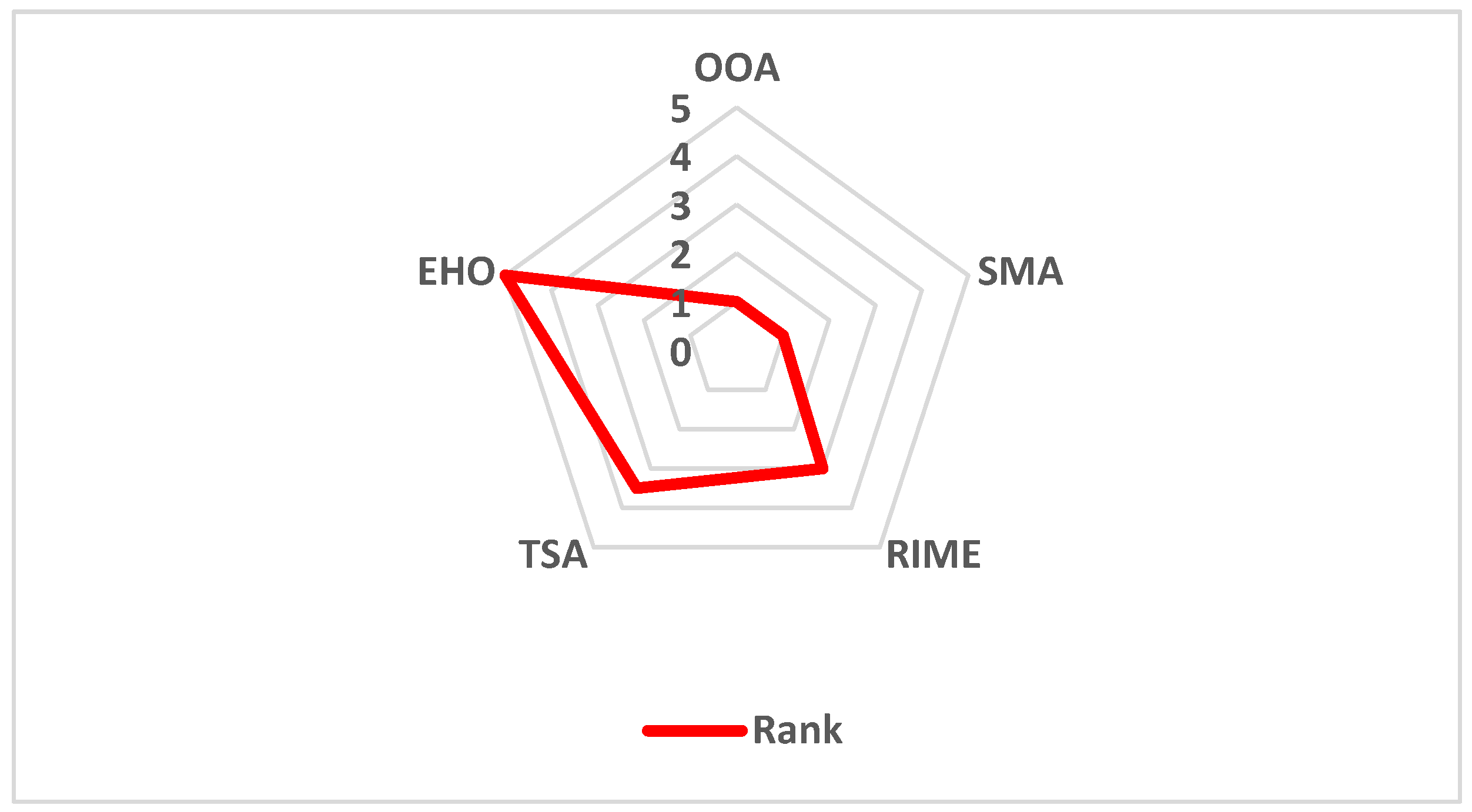
- The proposed OOA method is compared with the rime-ice algorithm (RIME), the tunicate swarm algorithm (TSA), the slime mould algorithm (SMA), and elephant herding optimization (EHO) for the same case study.
2. Economic Load Dispatch Problem
2.1. ELD
2.2. CEED
3. Osprey Optimization Algorithm
3.1. Inspiration of OOA
3.2. Mathematical Modelling
3.2.1. Initialization
3.2.2. Phase 1: Identification of Positions and Hunting of Fish (Exploration)
3.2.3. Phase 2: Carrying the Fish to the Suitable Location Position (Exploitation)
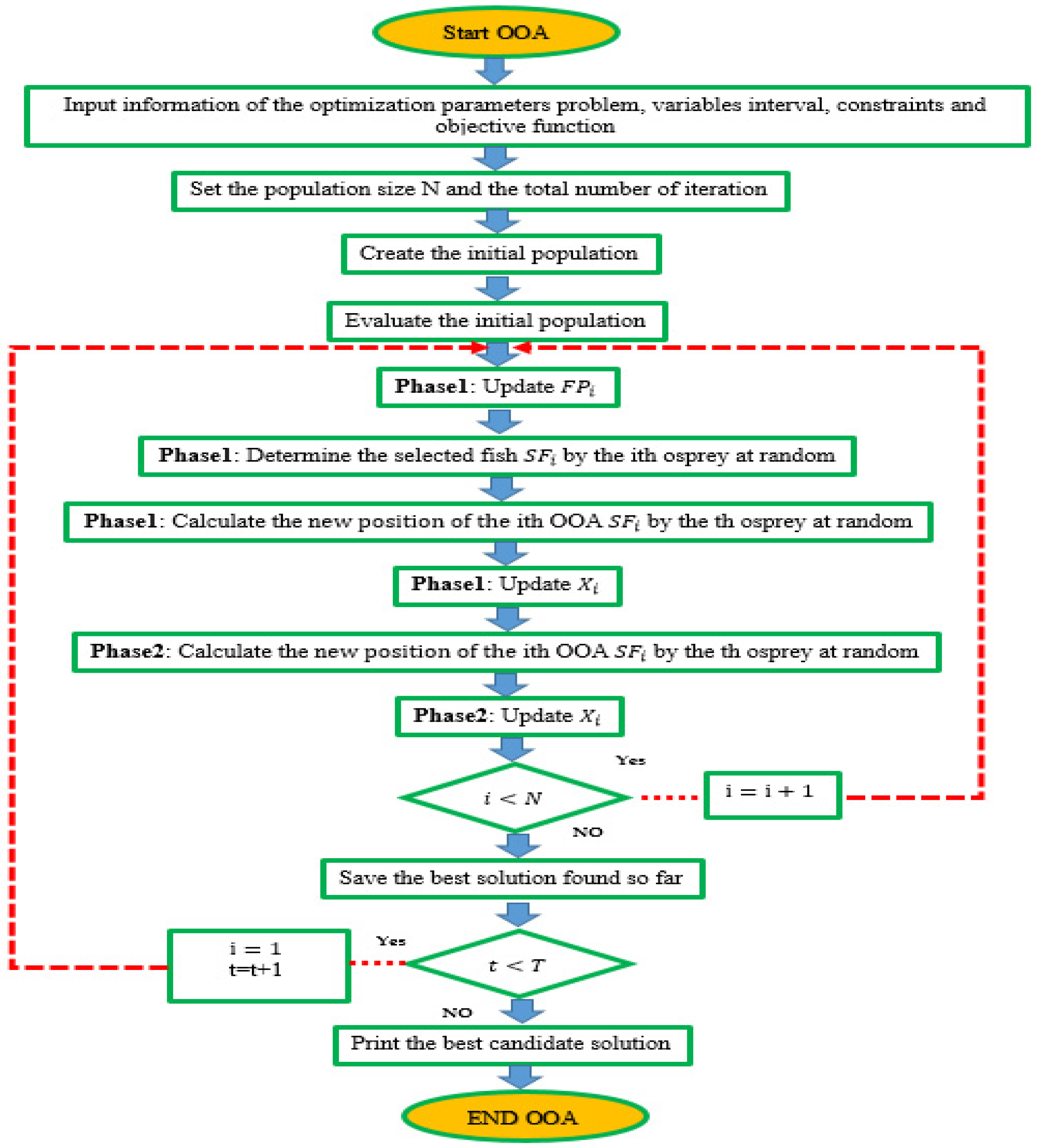
3.3. Repetition Process, Flowchart, and Pseudocode of OOA
4. Analysis and Discussion of Results
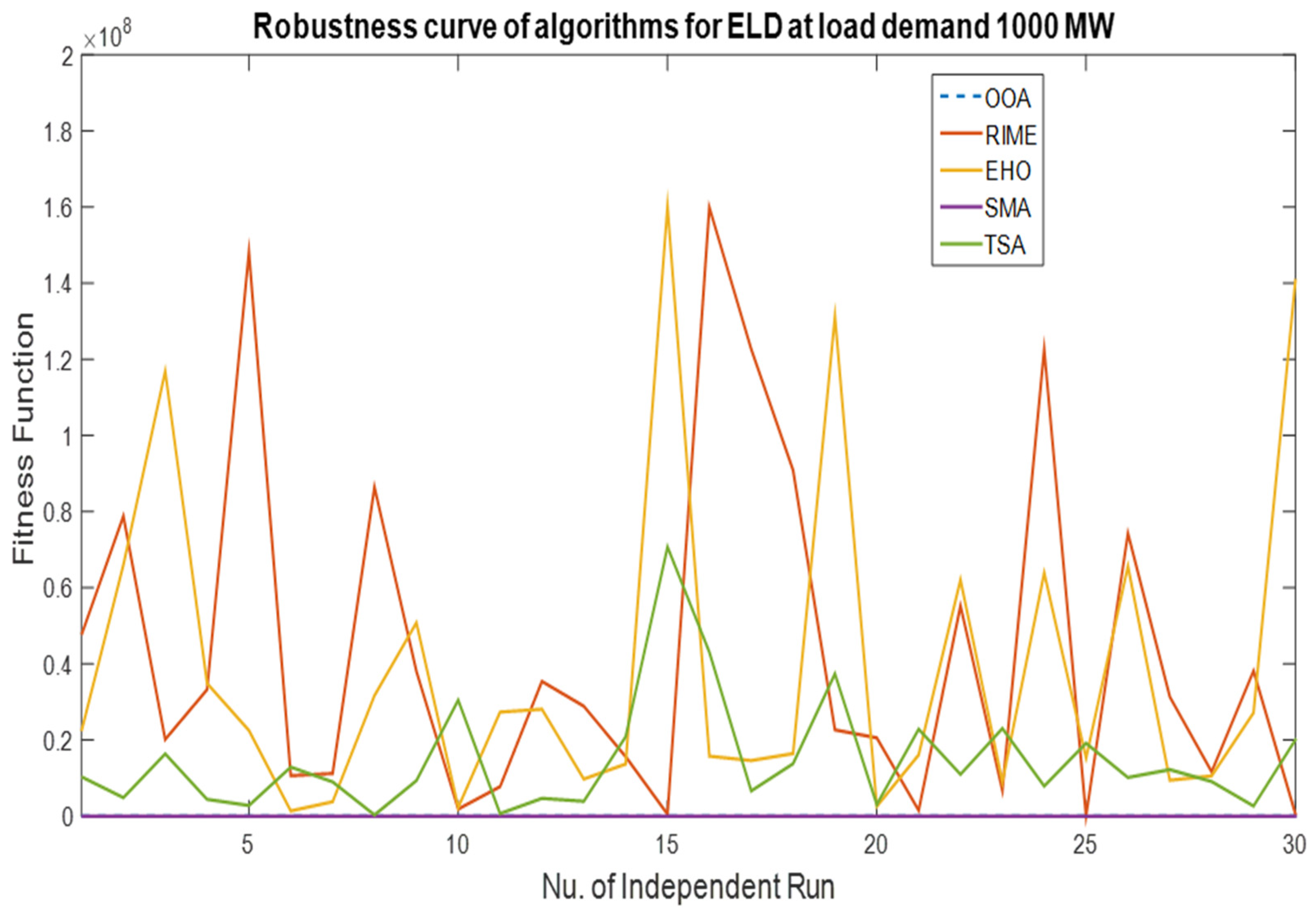
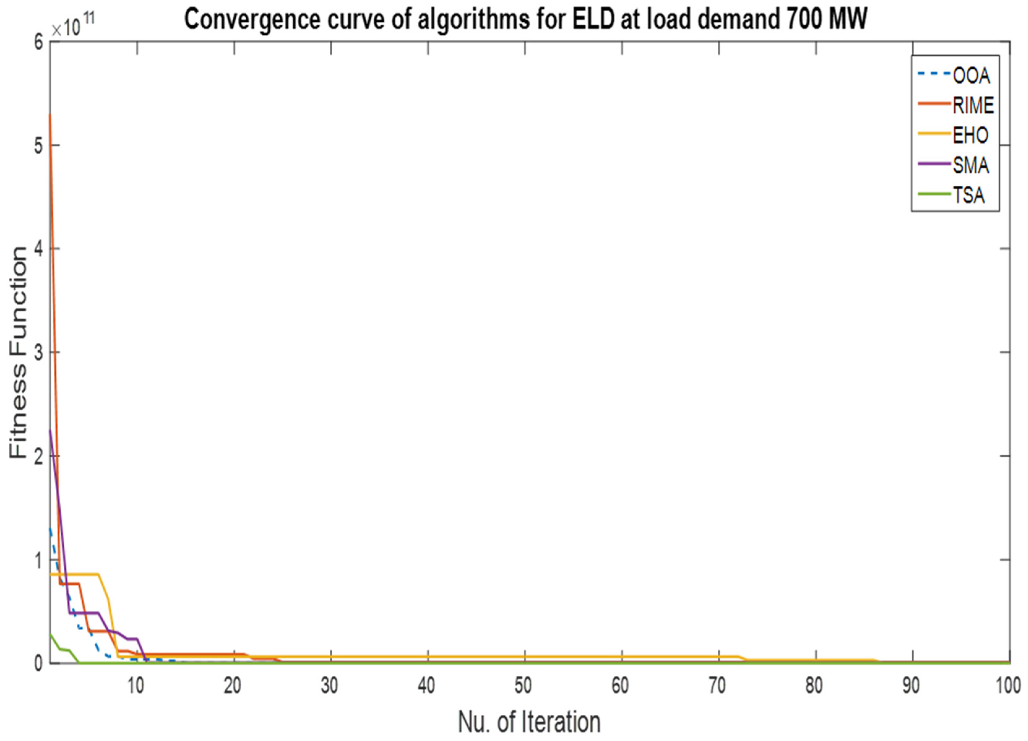
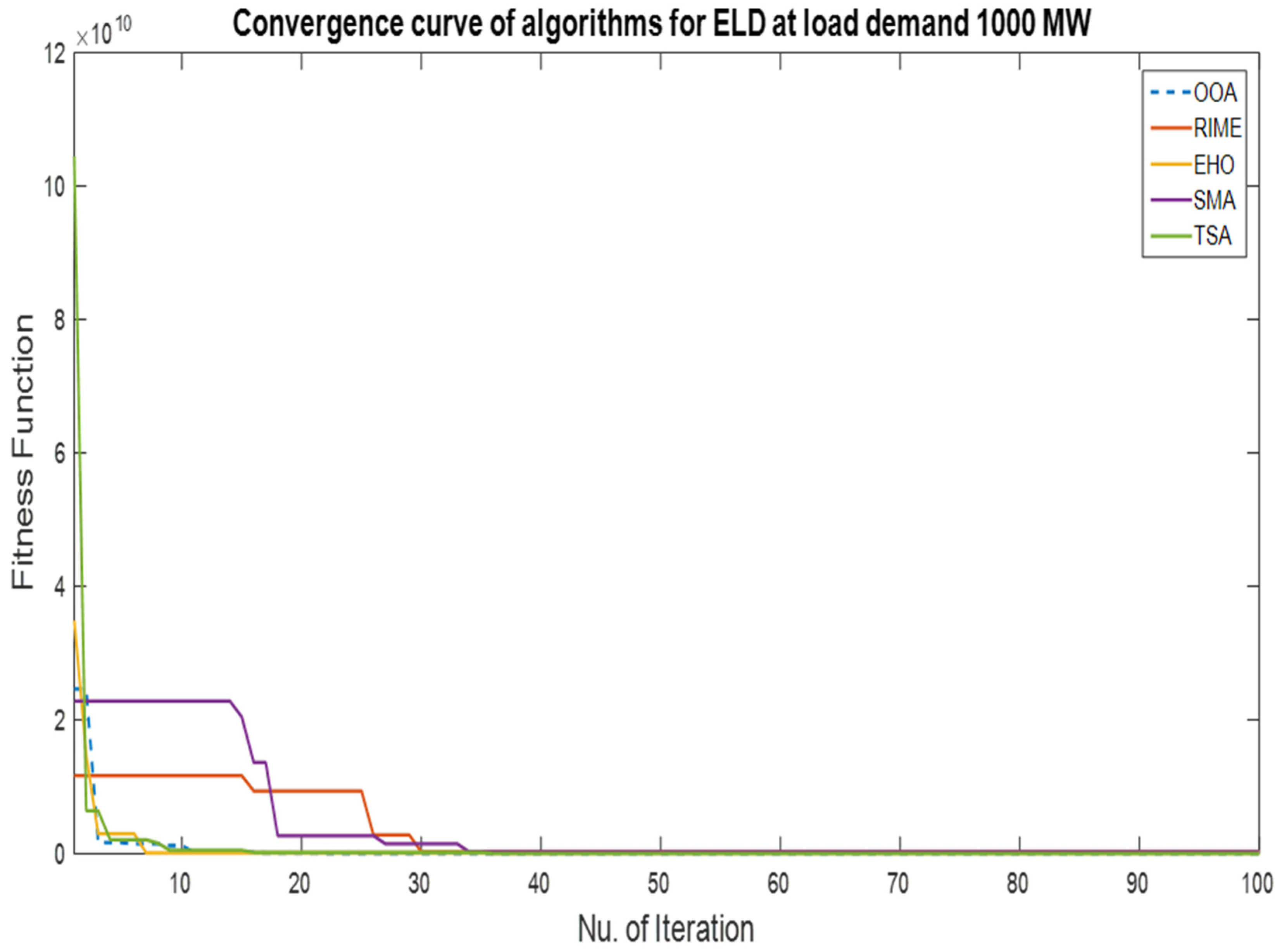
4.1. Results of ELD Issue
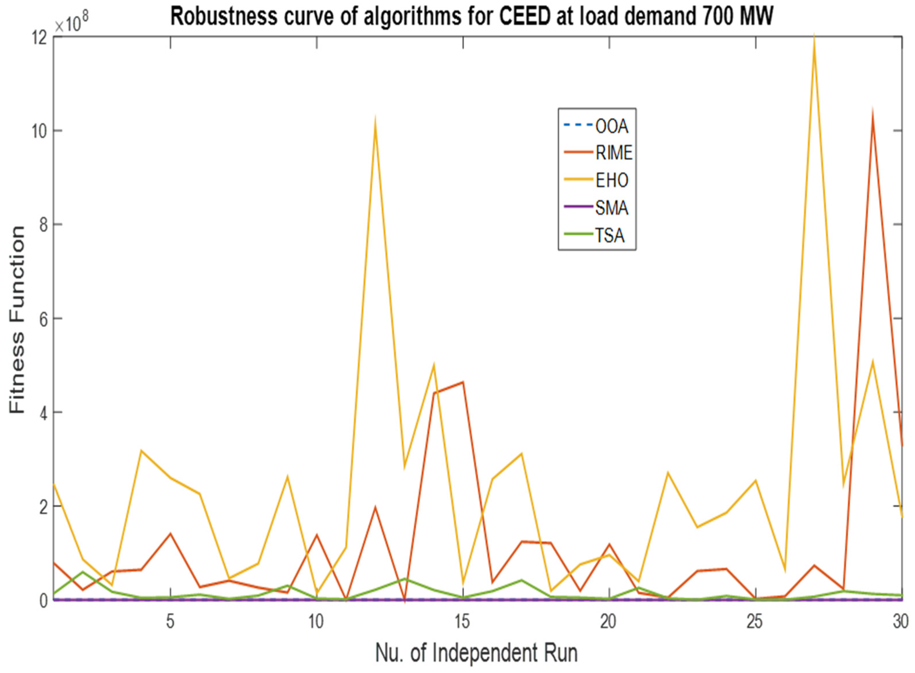
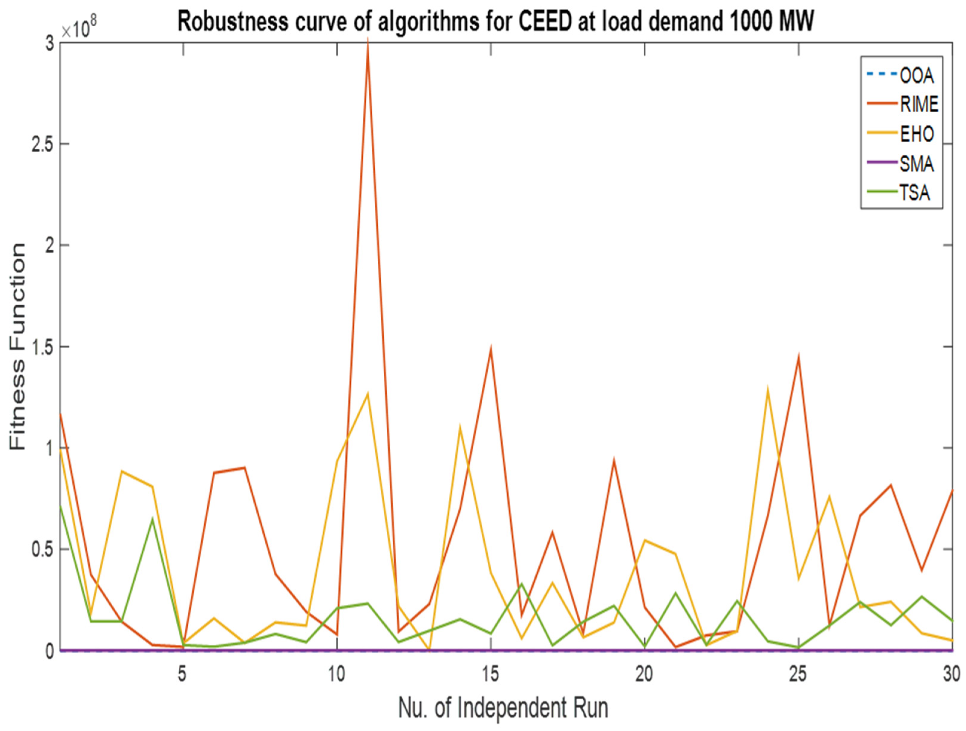
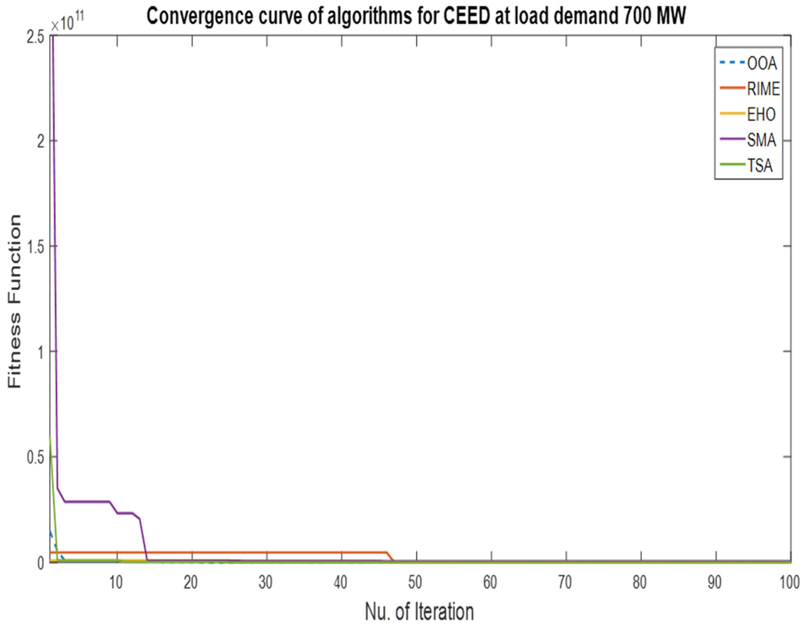
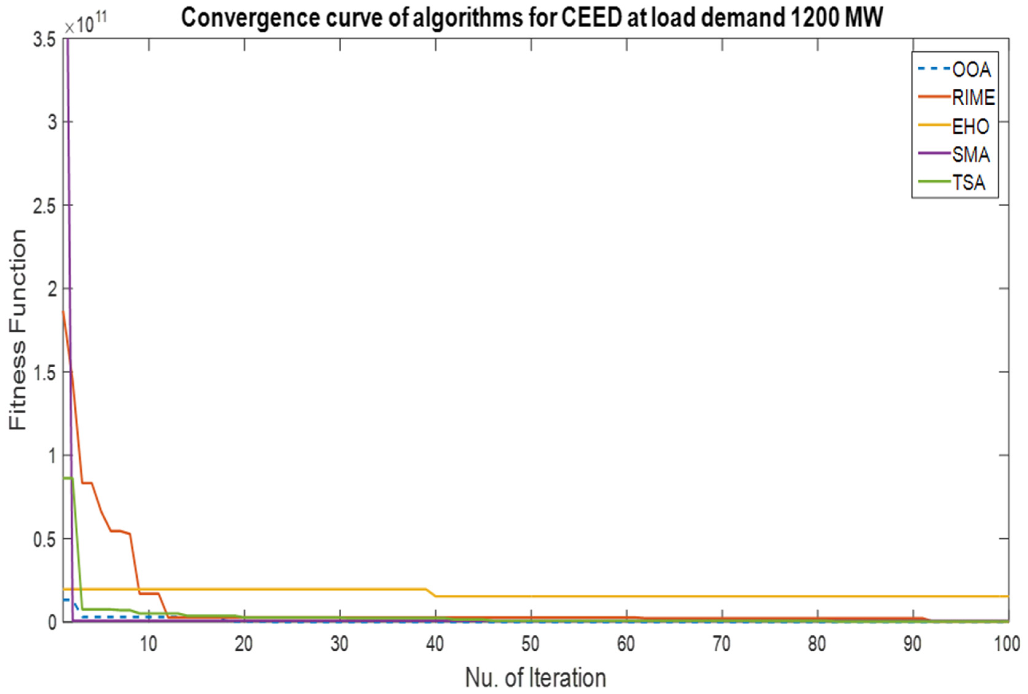
4.2. Results of CEED Problem
4.3. Discussion
5. Conclusions
Author Contributions
Funding
Data Availability Statement
Acknowledgments
Conflicts of Interest
References
- AbdElminaam, D.S.; Houssein, E.H.; Said, M.; Oliva, D.; Nabil, A. An efficient heap-based optimizer for parameters identification of modified photovoltaic models. Ain Shams Eng. J. 2022, 13, 101728. [Google Scholar] [CrossRef]
- Ismaeel, A.A.K.; Houssein, E.H.; Oliva, D.; Said, M. Gradient-based optimizer for parameter extraction in photovoltaic models. IEEE Access 2021, 9, 13403–13416. [Google Scholar] [CrossRef]
- Houssein, E.H.; Deb, S.; Oliva, D.; Rezk, H.; Alhumade, H.; Said, M. Performance of gradient-based optimizer on charging station placement problem. Mathematics 2021, 9, 2821. [Google Scholar] [CrossRef]
- Abdelminaam, D.S.; Said, M.; Houssein, E.H. Turbulent flow of water-based optimization using new objective function for parameter extraction of six photovoltaic models. IEEE Access 2021, 9, 35382–35398. [Google Scholar] [CrossRef]
- Said, M.; Houssein, E.H.; Deb, S.; Alhussan, A.A.; Ghoniem, R.M. A novel gradient-based optimizer for solving unit commitment problem. IEEE Access 2022, 10, 18081–18092. [Google Scholar] [CrossRef]
- Farag, A.; Al-Baiyat, S.; Cheng, T.C. Economic load dispatch multi-objective optimization procedures using linear programming techniques. IEEE Trans. Power Syst. 1995, 10, 731–738. [Google Scholar] [CrossRef]
- Al-Sumait, J.S.; Al-Othman, A.K.; Sykulski, J.K. Application of pattern search method to power system valve point economic load dispatch. Electr. Power Energy Syst. 2007, 29, 720–730. [Google Scholar] [CrossRef]
- Panigrahi, B.; Pandi, V.R.; Das, S. Adaptive particle swarm optimization approach for static and dynamic economic load dispatch. Energy Convers. Manag. 2008, 49, 1407–1415. [Google Scholar] [CrossRef]
- Aoki, K.; Satoh, T. Economic dispatch with network security constraints using parametric quadratic programming. IEEE Trans. Power Appar. Syst. 1982, 101, 4548–4556. [Google Scholar] [CrossRef]
- Braik, M.; Hammouri, A.; Atwan, J.; Al-Betar, M.A.; Awadallah, M.A. White shark optimizer: A novel bio-inspired metaheuristic algorithm for global optimization problems. Knowl. Based Syst. 2022, 243, 108457. [Google Scholar] [CrossRef]
- Said, M.; Houssein, E.H.; Deb, S.; Ghoniem, R.M.; Elsayed, A.G. Economic Load Dispatch Problem Based on Search and Rescue Optimization Algorithm. IEEE Access 2022, 10, 47109–47123. [Google Scholar] [CrossRef]
- Alghamdi, A.S. Greedy Sine-Cosine Non-Hierarchical Grey Wolf Optimizer for Solving Non-Convex Economic Load Dispatch Problems. Energies 2022, 15, 3904. [Google Scholar] [CrossRef]
- Said, M.; El-Rifaie, A.M.; Tolba, M.A.; Houssein, E.H.; Deb, S. An Efficient Chameleon Swarm Algorithm for Economic Load Dispatch Problem. Mathematics 2021, 9, 2770. [Google Scholar] [CrossRef]
- Al-Betar, M.A.; Awadallah, M.A.; Zitar, R.A.; Assaleh, K. Economic load dispatch using memetic sine cosine algorithm. J. Ambient. Intell. Humaniz. Comput. 2022, 14, 11685–11713. [Google Scholar] [CrossRef]
- Al-Betar, M.A.; Awadallah, M.A.; Makhadmeh, S.N.; Abu Doush, I.; Abu Zitar, R.; Alshathri, S.; Abd Elaziz, M. A hybrid Harris Hawks optimizer for economic load dispatch problems. Alex. Eng. J. 2023, 64, 365–389. [Google Scholar] [CrossRef]
- Ramalingam, R.; Karunanidy, D.; Alshamrani, S.S.; Rashid, M.; Mathumohan, S.; Dumka, A. Oppositional Pigeon-Inspired Optimizer for Solving the Non-Convex Economic Load Dispatch Problem in Power Systems. Mathematics 2022, 10, 3315. [Google Scholar] [CrossRef]
- Kaur, A.; Singh, L.; Dhillon, J.S. Modified Krill Herd Algorithm for constrained economic load dispatch problem. Int. J. Ambient. Energy 2022, 43, 4332–4342. [Google Scholar] [CrossRef]
- Andrade, G.L.; Schepke, C.; Lucca, N.; Neto, J.P.J. Modified Differential Evolution Algorithm Applied to Economic Load Dispatch Problems. In Computational Science and Its Applications ICCSA 2023; ICCSA 2023. Lecture Notes in Computer Science; Springer: Cham, Switzerland, 2023; Volume 13956. [Google Scholar]
- Bhattacharjee, K.; Shah, K.; Soni, J. Solving Economic Dispatch using Artificial Eco System-based Optimization. Electr. Power Compon. Syst. 2021, 49, 1034–1051. [Google Scholar] [CrossRef]
- Deb, S.; Houssein, E.H.; Said, M.; Abdelminaam, D.S. Performance of Turbulent Flow of Water Optimization on Economic Load Dispatch Problem. IEEE Access 2021, 9, 77882–77893. [Google Scholar] [CrossRef]
- Gaing, Z.-L. Particle swarm optimization to solving the economic dispatch considering the generator constraints. IEEE Trans. Power Syst. 2003, 18, 1187–1195. [Google Scholar] [CrossRef]
- Choi, K.; Jang, D.-H.; Kang, S.-I.; Lee, J.-H.; Chung, T.-K.; Kim, H.-S. Hybrid algorithm combing genetic algorithm with evolution strategy for antenna design. IEEE Trans. Magn. 2015, 52, 1–4. [Google Scholar] [CrossRef]
- Banerjee, S.; Maity, D.; Chanda, C.K. Teaching learning based optimization for economic load dispatch problem considering valve point loading effect. Int. J. Electr. Power Energy Syst. 2015, 73, 456–464. [Google Scholar] [CrossRef]
- Secui, D.C. A modified Symbiotic Organisms Search algorithm for large scale economic dispatch problem with valve-point effects. Energy 2016, 113, 366–384. [Google Scholar] [CrossRef]
- Selvakumar, A.I.; Thanushkodi, K. Optimization using civilized swarm: Solution to economic dispatch with multiple minima. Electr. Power Syst. Res. 2009, 79, 8–16. [Google Scholar] [CrossRef]
- Van, T.P.; Snasel, V.; Nguyen, T.T. Antlion optimization algorithm for optimal non-smooth economic load dispatch. Int. J. Electr. Comput. Eng. 2020, 10, 1187. [Google Scholar] [CrossRef]
- Cui, S.; Wang, Y.-W.; Lin, X.; Liu, X.-K. Distributed auction optimization algorithm for the nonconvex economic dispatch problem based on the gossip communication mechanism. Int. J. Electr. Power Energy Syst. 2018, 95, 417–426. [Google Scholar] [CrossRef]
- Jayabarathi, T.; Raghunathan, T.; Adarsh, B.R.; Suganthan, P.N. Economic dispatch using hybrid grey wolf optimizer. Energy 2016, 111, 630–641. [Google Scholar] [CrossRef]
- Chiang, C.-L. Improved Genetic Algorithm for Power Economic Dispatch of Units with Valve-Point Effects and Multiple Fuels. IEEE Trans. Power Syst. 2005, 20, 1690–1699. [Google Scholar] [CrossRef]
- Nguyen, T.T.; Quynh, N.V.; Van Dai, L. Improved Firefly Algorithm: A Novel Method for Optimal Operation of Thermal Generating Units. Complexity 2018, 2018, 7267593. [Google Scholar] [CrossRef]
- Bhattacharya, A.; Chattopadhyay, P.K. Biogeography-Based Optimization for Different Economic Load Dispatch Problems. IEEE Trans. Power Syst. 2010, 25, 1064–1077. [Google Scholar] [CrossRef]
- Hazra, A.; Das, S.; Laddha, A.; Basu, M. Economic Power Generation Strategy for Wind Integrated Large Power Network Using Heat Transfer Search Algorithm. J. Inst. Eng. Ser. B 2020, 101, 15–21. [Google Scholar] [CrossRef]
- Zakian, P.; Kaveh, A. Economic dispatch of power systems using an adaptive charged system search algorithm. Appl. Soft Comput. 2018, 73, 607–622. [Google Scholar] [CrossRef]
- Farhan Tabassum, M.; Saeed, M.; Ahmad Chaudhry, N.; Ali, J.; Farman, M.; Akram, S. Evolutionary simplex adaptive HookeJeeves algorithm for economic load dispatch problem considering valve point loading effects. Ain Shams Eng. J. 2021, 12, 1001–1015. [Google Scholar] [CrossRef]
- Elsakaan, A.A.; El-Sehiemy, R.A.; Kaddah, S.S.; Elsaid, M.I. An enhanced moth-flame optimizer for solving non-smooth economic dispatch problems with emissions. Energy 2018, 157, 1063–1078. [Google Scholar] [CrossRef]
- Xiong, G.; Shi, D.; Duan, X. Multi-strategy ensemble biogeography based optimization for economic dispatch problems. Appl. Energy 2013, 111, 801–811. [Google Scholar] [CrossRef]
- Vaisakh, K.; Reddy, A.S. MSFLA/GHS/SFLA-GHS/SDE algorithms for economic dispatch problem considering multiple fuels and valve point loadings. Appl. Soft Comput. 2013, 13, 4281–4291. [Google Scholar] [CrossRef]
- Elsayed, W.T.; El-Saadany, E.F. A Fully Decentralized Approach for Solving the Economic Dispatch Problem. IEEE Trans. Power Syst. 2015, 30, 2179–2189. [Google Scholar] [CrossRef]
- Ghorbani, N.; Babaei, E. Exchange market algorithm for economic load dispatch. Int. J. Electr. Power Energy Syst. 2016, 75, 19–27. [Google Scholar] [CrossRef]
- Panigrahi, B.K.; Ravikumar Pandi, V. Bacterial foraging optimisation: Nelder–Mead hybrid algorithm for economic load dispatch. IET Gener. Transm. Distrib. 2008, 2, 556. [Google Scholar] [CrossRef]
- Kaboli, S.H.A.; Alqallaf, A.K. Solving non-convex economic load dispatch problem via artificial cooperative search algorithm. Expert Syst. Appl. 2019, 128, 14–27. [Google Scholar] [CrossRef]
- Kapelinski, K.; Neto, J.P.J.; dos Santos, E.M. Firefly Algorithm with non-homogeneous population: A case study in economic load dispatch problem. J. Oper. Res. Soc. 2021, 72, 519–534. [Google Scholar] [CrossRef]
- Shayeghi, H.; Ghasemi, A. A modified artificial bee colony based on chaos theory for solving non-convex emission/economic dispatch. Energy Convers. Manag. 2014, 79, 344–354. [Google Scholar] [CrossRef]
- Binetti, G.; Davoudi, A.; Naso, D.; Turchiano, B.; Lewis, F.L. A Distributed Auction-Based Algorithm for the Nonconvex Economic Dispatch Problem. IEEE Trans. Ind. Inform. 2014, 10, 1124–1132. [Google Scholar] [CrossRef]
- Nguyen, T.T.; Vo, D.N. The application of one rank cuckoo search algorithm for solving economic load dispatch problems. Appl. Soft Comput. 2015, 37, 763–773. [Google Scholar] [CrossRef]
- Mohammadi, F.; Abdi, H.A. modified crow search algorithm (MCSA) for solving economic load dispatch problem. Appl. Soft Comput. 2018, 71, 51–65. [Google Scholar] [CrossRef]
- Ho, Y.C.; Pepyne, D.L. Simple explanation of the no-free-lunch theorem and its implications. J. Optim. Theory Appl. 2002, 115, 549–570. [Google Scholar] [CrossRef]
- Adam, S.P.; Alexandropoulos, S.A.N.; Pardalos, P.M.; Vrahatis, M.N. No free lunch theorem: A review. In Approximation and Optimization: Algorithms, Complexity and Applications; Springer: Berlin/Heidelberg, Germany, 2019; pp. 57–82. [Google Scholar]
- Whitley, D.; Watson, J.P. Complexity theory and the no free lunch theorem. In Search Methodologies; Springer: Berlin/Heidelberg, Germany, 2005; pp. 317–339. [Google Scholar]
- Dohmatob, E. Generalized no free lunch theorem for adversarial robustness. In Proceedings of the International Conference on Machine Learning, Long Beach, CA, USA, 9–15 June 2019; pp. 1646–1654. [Google Scholar]
- Hanneke, S.; Kpotufe, S. A no-free-lunch theorem for multitask learning. arXiv 2020, arXiv:2006.15785. [Google Scholar] [CrossRef]
- Dehghani, M.; Trojovský, P. Osprey optimization algorithm: A new bioinspired metaheuristic algorithm for solving engineering optimisation problems. Front. Mech. Eng. 2023, 8, 1126450. [Google Scholar] [CrossRef]
- Kaur, S.; Awasthi, L.K.; Sangal, A.L.; Dhiman, G. Tunicate Swarm Algorithm: A new bio-inspired based metaheuristic paradigm for global optimization. Eng. Appl. Artif. Intell. 2020, 90, 103541. [Google Scholar] [CrossRef]
- Hang, S.; Zhao, D.; Heidari, A.A.; Liu, L.; Zhang, X.; Mafarja, M.; Chen, H. RIME: A physics-based optimization. Neurocomputing 2023, 532, 183–214. [Google Scholar]
- Shimin, L.; Chen, H.; Wang, M.; Heidari, A.A.; Mirjalili, S. Slime mould algorithm: A new method for stochastic optimization. Future Gener. Comput. Syst. 2020, 111, 300–323. [Google Scholar]
- Wang, G.G.; Deb, S.; Coelho, L.D. Elephant herding optimization. In Proceedings of the 2015 3rd IEEE International Symposium on Computational and Business Intelligence (ISCBI), Bali, Indonesia, 7–9 December 2015; pp. 1–5. [Google Scholar]


| Year | Reference | Description |
|---|---|---|
| 2003 | [21] | The EED problem was solved using the PSO method while taking into account generator limitations such as ramp rate limits and prohibited operation zones. |
| 2005 | [29] | Power economic dispatch problems were solved using an IGA, and it was tested using three different scenarios: one that considered valve-point effects, one that considered various fuels, and one that addressed both valve-point effects and numerous fuels. |
| 2008 | [40] | Non-convex ED problems with a variety of restrictions may be solved with ease by the Nelder-Mead hybrid technique. Simulations of several standard test systems with variable numbers of generating units were run. |
| 2009 | [25] | A series of multi-minima economic dispatch problems were used to evaluate the performance of CSO. |
| 2010 | [31] | Convex and non-convex ELD problems facing thermal plants were solved using a BBO method. This approach was applied to four different test systems, both small and big, requiring differing degrees of complexity. |
| 2013 | [36] | For resolving ELD problems, the authors suggested a MSEBBO. The no free lunch theorem is used by the MEEBBO to enhance the three elements of BBO to maintain a good balance between exploration and exploitation. Additionally, a powerful repair method is suggested to address the various ELD problem constraints. |
| 2014 | [43] | The standard IEEE 30 bus with six generators, fourteen generators, and forty thermal generating units was subjected to the modified artificial bee colony approach for non-convex CEED problems. |
| 2014 | [44] | The non-convex ELD problem was solved using a distributed auction-based method and had many constraints, including the valve-point loading effect, numerous fuel alternatives, and restricted operating zones. |
| 2015 | [23] | To solve EPLD problems while considering transmission losses, the TLBO method was used. This method explores the solution space for the global optimal point. |
| 2015 | [38] | The non-convex formulation of the ED problem can be solved very efficiently using a DA method, and transmission losses can be precisely taken into consideration in a fully decentralized way. Three case studies were examined. |
| 2015 | [45] | ELD issues were solved with the ORCSA method. Additionally, complete testing on several systems with various restrictions and thermal unit characteristics was presented. |
| 2016 | [24] | Five systems—13-unit, 40-unit, 80-unit, 160-unit, and 320-unit systems—with various features, constraints, and dimensions were used to evaluate the performance of the MSOS. |
| 2016 | [28] | Using a HGWO, four economic dispatch problems with 6, 15, 40, and 80 generators were tested. |
| 2016 | [39] | The EMA is a reliable and effective technique for locating the global optimization’s best solution for ELD situations. Additionally, four test systems in four distinct dimensions—3, 6, 15, and 40 units—with both convex and non-convex cost functions—were used to develop it. |
| 2018 | [27] | The most effective approach for the ELD problem was discovered using the DAOA. |
| 2018 | [33] | Using an ACSS method, a variety of economic dispatch cases formed of 6-, 13-, 15-, 40-, 160-, and 640-unit generating systems were studied as benchmarks for small- and large-scale problems. |
| 2018 | [35] | The non-convex ELD problem with valve-point effects and emissions was solved using the EMFO method on three typical test systems comprising 6, 40, and a large-scale 80 generating units with non-convex fuel cost functions. |
| 2018 | [46] | The non-convex ELD problem was solved using the MCSA and applied to five well-known test systems. |
| 2019 | [41] | The ACS technique, based on a co-evolutionary technique, was offered as a potential solution to the challenging ELD problem. |
| 2020 | [26] | Problems involving the optimal ELD were handled using the ALO. The results of applying the ALO algorithm to all three cases revealed that it has greater potential than other techniques for the solution, stability, and convergence velocity. |
| 2020 | [32] | The HT method was used to resolve the complex ELD problem with the integration of wind generation. |
| 2021 | [13] | The ELD problem was resolved based on CSA’s effective operation with a six-unit system. |
| 2021 | [20] | To solve ELD and CEED issues, the authors created a TFWO method. |
| 2021 | [34] | On five generating systems with valve-point effects, the ESAHJ performance was evaluated. The test findings for the suggested approach showed high convergence features and low generation costs, making them extremely effective and encouraging. |
| 2021 | [42] | ELD problems were solved with the FA. A 15-unit ELD problem with many considerations for each generator was solved using ten benchmark functions, and a 13-unit non-convex system with a valve-point loading effect was solved. |
| 2022 | [11] | The SAR was used by the authors to get at the optimum approach for the CEED and ELD. The outcomes demonstrated that the SAR was the optimum option for ELD, integrated pollution control, and economic dispatch. |
| 2022 | [12] | To solve ELD problems, the authors proposed a GSCGWO. The power generators in these four power systems total 10, 15, 40, and 140, with various valuation times. |
| 2022 | [16] | The ELD problem of small-scale (13-unit, 40-unit), medium-scale (140-unit, 160-unit), and large-scale (320-unit, 640-unit) test systems was solved using the OPIO algorithm. |
| 2022 | [17] | The authors solved an ELD issue with the MKH method. In comparison to other metaheuristics, the MKH was found to perform rather well, and tweaking parameters in the MKH was also fairly simple. |
| 2023 | [14] | The ELD problem was solved by a memetic sine cosine algorithm that was applied to six real-world cases: 3, 6, 13, 13, 15, and 40 units of generator. |
| 2023 | [15] | ELD problems were solved using HHO methods in six generation units. |
| 2023 | [18] | The global minimum and other instances of the ELD were obtained by solving a series of test functions using the modified differential evolution method. |
| Algorithms | Parameter Setting |
|---|---|
| General setting | No. of iterations = 1000 Decision parameters = 6 Population size = 30 |
| OOA | ri,j are random numbers in the interval [0, 1], Ii,j are random numbers from the set {1, 2} |
| RIME | r1, and r3 are random numbers within (−1, 1) r2 is a random number in the range (0, 1) |
| EHO | alpha = 0.5, beta = 0.1 |
| SMA | Z = 0.03 |
| TSA | Pmin = 1 and Pmax = 4 |
| Demand (MW) | Algorithm | Min | SD | Mean | Max |
|---|---|---|---|---|---|
| 700 | OOA | 8489.71013 | 5,076,187.167 | 935,505.3799 | 27,812,146.81 |
| RIME | 157,119.6598 | 56,610,134.62 | 52,654,562.24 | 190,938,550.9 | |
| EHO | 323,503.0771 | 164,951,021.9 | 157,742,034.9 | 830,026,118.4 | |
| SMA | 8502.406541 | 898.1936009 | 9689.146486 | 12,698.30255 | |
| TSA | 161,424.5504 | 1.25 × 10⁷ | 11,045,846.26 | 43,283,357.63 | |
| 1000 | OOA | 12,145.56118 | 147.1792166 | 12,328.60609 | 12,769.69945 |
| RIME | 43,804.62747 | 45,918,517.41 | 44,117,668.43 | 159,925,064.1 | |
| EHO | 1,385,818.233 | 43,729,545 | 39,739,552.31 | 160,205,265 | |
| SMA | 12,310.85263 | 3167.418523 | 13,720.89249 | 29,123.65877 | |
| TSA | 338,416.1136 | 1.49 × 10⁷ | 14,797,087.09 | 70,710,421.98 | |
| 1200 | OOA | 14,844.17028 | 106,377.3814 | 34,559.66353 | 597,774.5881 |
| RIME | 647,657.0993 | 111,021,190.9 | 76,380,860.23 | 557,699,468.3 | |
| EHO | 66,594,721.86 | 2,050,678,201 | 2,246,833,875 | 8,220,483,497 | |
| SMA | 14,960.25669 | 2462.012063 | 16,065.99129 | 27,329.59533 | |
| TSA | 1,040,954.65 | 21,439,850.48 | 23,898,498.47 | 65,710,037.14 |
| Algorithm | 700 MW | 1000 MW | 1200 MW |
|---|---|---|---|
| OOA | 8489.71013 | 12,145.56118 | 14,844.17028 |
| RIME | 8930.126895 | 12,220.14976 | 14,929.15938 |
| EHO | 9201.247567 | 13,577.96384 | 17,159.01262 |
| SMA | 8502.406541 | 12,269.08288 | 14,890.22354 |
| TSA | 8719.411543 | 12,324.03706 | 15,043.25053 |
| OOA | RIME | EHO | SMA | TSA |
|---|---|---|---|---|
| 288.1936492 | 100 | 74.27685394 | 291.9724948 | 179.5604411 |
| 71.24189189 | 97.67174678 | 96.60780328 | 95.58202252 | 68.62630472 |
| 94.19305375 | 172.6253448 | 108.0508678 | 96.94958415 | 120.8437852 |
| 77.62559738 | 134.7024241 | 128.464386 | 66.84420361 | 133.2068048 |
| 101.6542888 | 112.6905922 | 151.8904691 | 97.50539107 | 161.4281797 |
| 78.76324794 | 96.46689215 | 153.8266087 | 62.48476668 | 50 |
| OOA | RIME | EHO | SMA | TSA |
|---|---|---|---|---|
| 400.5765793 | 416.3680247 | 89.88251423 | 413.3002088 | 499.1064857 |
| 184.3641601 | 58.65210153 | 115.9348269 | 199.8242953 | 56.13947257 |
| 198.9629992 | 247.8243991 | 136.9111861 | 186.8499139 | 144.1194586 |
| 60.51914068 | 107.9181452 | 145.4592182 | 51.97368989 | 138.9537992 |
| 124.4995504 | 95.19702846 | 208.9981201 | 50.99369441 | 114.1379038 |
| 54.35074684 | 98.1158557 | 327.7323289 | 119.9990952 | 70.12055135 |
| OOA | RIME | EHO | SMA | TSA |
|---|---|---|---|---|
| 468.1992937 | 500 | 76.71759497 | 415.970695 | 500 |
| 183.9250281 | 90.28209597 | 113.5295062 | 168.0667693 | 190.1559272 |
| 248.0430036 | 247.1131882 | 179.1731727 | 298.2491761 | 122.6292221 |
| 97.982237 | 123.8746742 | 181.4297643 | 104.1223325 | 128.515068 |
| 169.116858 | 157.7756826 | 192.5547606 | 199.9999955 | 173.3199231 |
| 67.2444517 | 115.9580053 | 491.0321006 | 50.06577066 | 120 |
| Demand (MW) | Algorithm | Min | SD | Mean | Max |
|---|---|---|---|---|---|
| 700 | OOA | 13,729.25276 | 451.5174275 | 14,516.06635 | 15,328.15021 |
| RIME | 192,447.3458 | 208,328,375.9 | 124,827,189.5 | 1,026,320,992 | |
| EHO | 14,201,636.42 | 266,068,058.3 | 245,161,496.9 | 1,180,743,975 | |
| SMA | 13,902.65065 | 1346.302672 | 16,232.30745 | 20,837.35633 | |
| TSA | 437,640.1904 | 14,454,883.71 | 13,696,680.57 | 59,328,593.81 | |
| 1000 | OOA | 21,615.36632 | 942.8912121 | 22,726.61646 | 24,636.02763 |
| RIME | 1,716,313.573 | 62,284,621.82 | 55,672,191.78 | 295,816,509.5 | |
| EHO | 37,048.65857 | 40,394,801.02 | 39,978,221.4 | 128,249,578.6 | |
| SMA | 21,825.35037 | 2359.444736 | 24,422.15373 | 32,181.52154 | |
| TSA | 1,527,919.533 | 16,727,355.69 | 16,432,066.87 | 71,410,265.4 | |
| 1200 | OOA | 27,973.14804 | 51,923.65941 | 38,269.17284 | 313,175.7045 |
| RIME | 867,550.5025 | 64,850,599.89 | 64,743,277.09 | 222,328,197.6 | |
| EHO | 48,039,881.34 | 2,312,392,376 | 1,919,239,905 | 8,618,622,585 | |
| SMA | 28,405.56152 | 1902.826273 | 30,216.01233 | 36,613.94417 | |
| TSA | 231,004.4218 | 18,455,252.22 | 22,333,023.46 | 68,956,768.4 |
| Algorithm | 700 MW | 1000 MW | 1200 MW | |||
|---|---|---|---|---|---|---|
| Fuel | Emission | Fuel | Emission | Fuel | Emission | |
| OOA | 8483.634452 | 5588.646691 | 12,161.84094 | 10,233.44274 | 14,866.11098 | 14,612.79425 |
| RIME | 8431.695806 | 5047.42326 | 12,307.94781 | 13,121.02468 | 14,861.21847 | 15,743.05095 |
| EHO | 9206.302521 | 10,616.02658 | 13,814.47332 | 27,920.96174 | 17,437.93278 | 50,362.10471 |
| SMA | 8507.728643 | 6105.614158 | 12,188.25965 | 9816.166095 | 14,862.5486 | 15,868.57055 |
| TSA | 8776.708178 | 7371.129746 | 12,381.47358 | 10,375.96202 | 14,920.81305 | 18,329.33556 |
| OOA | RIME | EHO | SMA | TSA |
|---|---|---|---|---|
| 269.767936 | 343.4755772 | 88.50987751 | 217.1592473 | 131.1911477 |
| 96.13075673 | 59.06883111 | 92.10828089 | 89.13670916 | 170.6718075 |
| 111.2458027 | 96.84808663 | 104.5033046 | 156.2882148 | 199.7174815 |
| 101.0842946 | 55.47194818 | 109.9641282 | 82.28373091 | 55.52645172 |
| 60.74111401 | 93.04112837 | 124.918835 | 96.78800842 | 72.68207485 |
| 72.43570158 | 63.01857975 | 192.5541969 | 70.63969799 | 83.47079715 |
| OOA | RIME | EHO | SMA | TSA |
|---|---|---|---|---|
| 365.8570453 | 346.5147003 | 87.1819096 | 357.847752 | 483.0745935 |
| 158.5402394 | 50 | 102.8530268 | 167.9022744 | 131.8231399 |
| 189.5613645 | 266.824565 | 102.8581958 | 202.5030352 | 101.8290821 |
| 110.3792318 | 85.95375207 | 134.8791731 | 50 | 146.1161231 |
| 115.2493189 | 200 | 247.0179056 | 166.607947 | 59.26627522 |
| 84.29429492 | 77.67398741 | 350.2591399 | 79.834013 | 99.95671992 |
| OOA | RIME | EHO | SMA | TSA |
|---|---|---|---|---|
| 449.6819234 | 494.9447771 | 52.0752919 | 494.283923 | 461.4678788 |
| 147.8653475 | 143.4837708 | 100.9132864 | 142.773607 | 104.8448432 |
| 243.9501883 | 278.0708989 | 131.3313064 | 270.2859306 | 300 |
| 99.5666135 | 107.0759198 | 177.0521457 | 135.9364431 | 100.5227517 |
| 195.2957655 | 155.8467164 | 290.5798172 | 139.9015771 | 149.014853 |
| 99.41554831 | 54.80297076 | 481.7029118 | 50.79427633 | 120 |
| Cases | Method | 700 MW | 1000 MW | 1200 MW |
|---|---|---|---|---|
| ELD | OOA | 7.64 × 10⁻¹³ | 7.50 × 10⁻¹³ | 4.26 × 10⁻¹³ |
| RIME | 1.48 × 10⁻⁵ | 3.16 × 10⁻⁶ | 6.33 × 10⁻⁵ | |
| EHO | 2.239431602 | 9.904979361 | 20.33855573 | |
| SMA | 5.61 × 10⁻⁹ | 4.18 × 10⁻⁹ | 7.00 × 10⁻⁹ | |
| TSA | 1.53 × 10⁻⁵ | 3.26 × 10⁻⁵ | 0.000102591 | |
| SCA [11] | 0.00076719 | 0.000182 | 0.00154 | |
| MBO [11] | 2.338728225 | 20.33553784 | 13.5932468 | |
| ABC [11] | 8.85 × 10⁻⁵ | 0.000172518 | 0.000464669 | |
| MSA [11] | 8.164408631 | 16.26317 | 22.86726197 | |
| ChOA [11] | 0.000284475 | 0.000476787 | 1.28 × 10⁻⁵ | |
| CEED | OOA | 1.10 × 10⁻¹³ | 1.07 × 10⁻¹³ | 9.32 × 10⁻¹⁰ |
| RIME | 1.79 × 10⁻⁵ | 0.000169392 | 8.39 × 10⁻⁵ | |
| EHO | 2.939436145 | 11.67444458 | 23.59139609 | |
| SMA | 2.52 × 10⁻⁸ | 5.57 × 10⁻⁹ | 2.29 × 10⁻⁸ | |
| TSA | 4.23 × 10⁻⁵ | 0.000150503 | 2.03 × 10⁻⁵ | |
| SCA [11] | 0.000128581 | 0.001259941 | 0.00153618 | |
| MBO [11] | 2.224948582 | 18.75789013 | 19.58822153 | |
| ABC [11] | 0.000176679 | 3.74 × 10⁻⁵ | 0.000402522 | |
| MSA [11] | 7.228241532 | 12.18295414 | 23.26274643 | |
| ChOA [11] | 0.000284475 | 0.000476787 | 6.47 × 10⁻⁵ |
Disclaimer/Publisher’s Note: The statements, opinions and data contained in all publications are solely those of the individual author(s) and contributor(s) and not of MDPI and/or the editor(s). MDPI and/or the editor(s) disclaim responsibility for any injury to people or property resulting from any ideas, methods, instructions or products referred to in the content. |
© 2023 by the authors. Licensee MDPI, Basel, Switzerland. This article is an open access article distributed under the terms and conditions of the Creative Commons Attribution (CC BY) license (https://creativecommons.org/licenses/by/4.0/).
Share and Cite
Ismaeel, A.A.K.; Houssein, E.H.; Khafaga, D.S.; Abdullah Aldakheel, E.; AbdElrazek, A.S.; Said, M. Performance of Osprey Optimization Algorithm for Solving Economic Load Dispatch Problem. Mathematics 2023, 11, 4107. https://doi.org/10.3390/math11194107
Ismaeel AAK, Houssein EH, Khafaga DS, Abdullah Aldakheel E, AbdElrazek AS, Said M. Performance of Osprey Optimization Algorithm for Solving Economic Load Dispatch Problem. Mathematics. 2023; 11(19):4107. https://doi.org/10.3390/math11194107
Chicago/Turabian StyleIsmaeel, Alaa A. K., Essam H. Houssein, Doaa Sami Khafaga, Eman Abdullah Aldakheel, Ahmed S. AbdElrazek, and Mokhtar Said. 2023. "Performance of Osprey Optimization Algorithm for Solving Economic Load Dispatch Problem" Mathematics 11, no. 19: 4107. https://doi.org/10.3390/math11194107
APA StyleIsmaeel, A. A. K., Houssein, E. H., Khafaga, D. S., Abdullah Aldakheel, E., AbdElrazek, A. S., & Said, M. (2023). Performance of Osprey Optimization Algorithm for Solving Economic Load Dispatch Problem. Mathematics, 11(19), 4107. https://doi.org/10.3390/math11194107