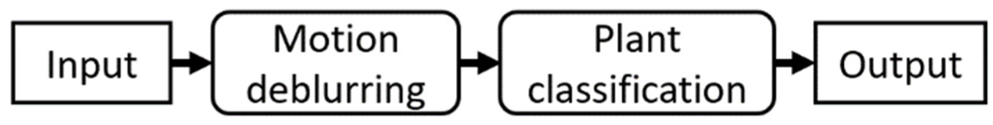
Figure 1.
Flowchart of the overall system.
Figure 1.
Flowchart of the overall system.
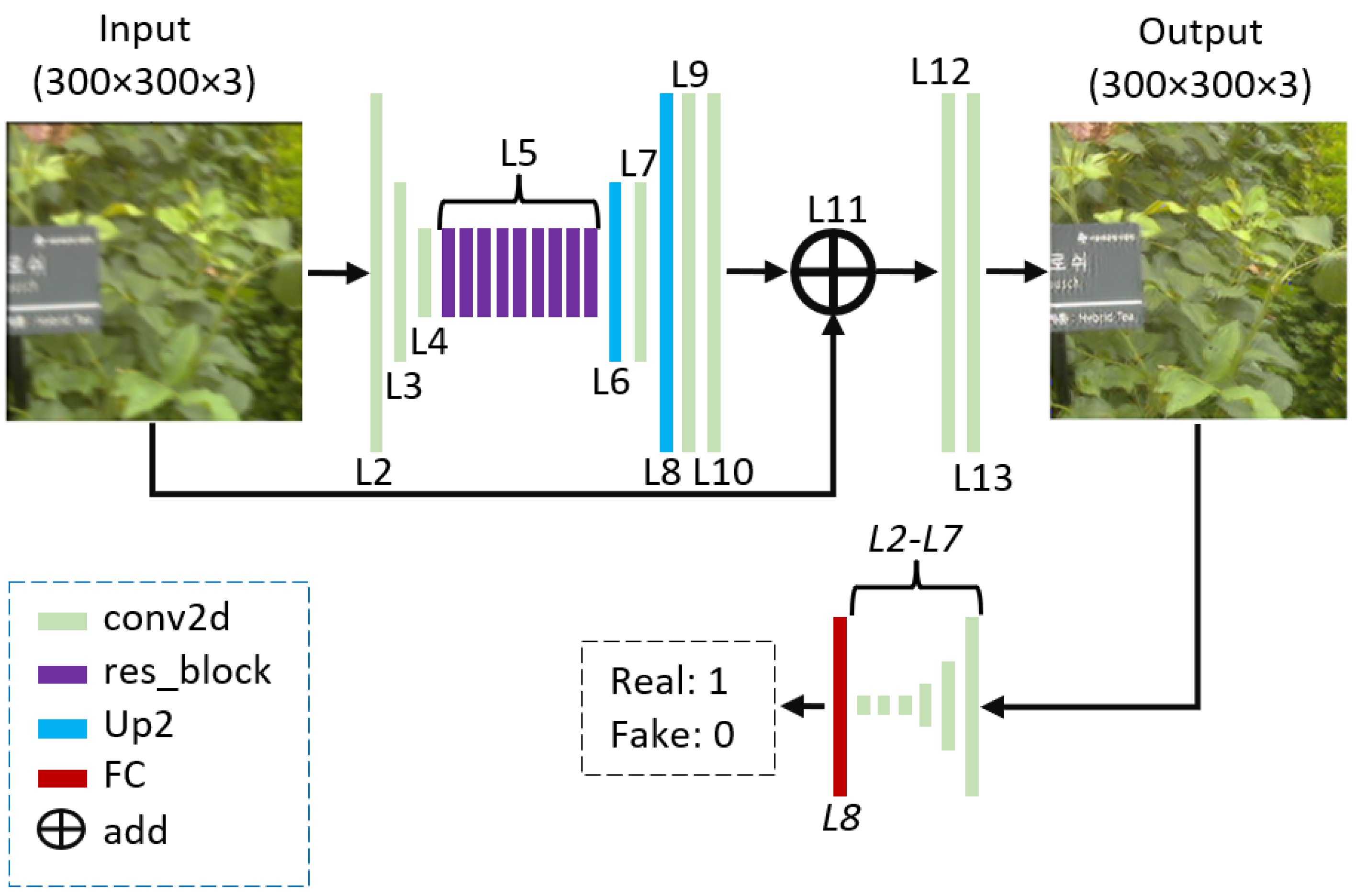
Figure 2.
Structure of the PI-NMD.
Figure 2.
Structure of the PI-NMD.
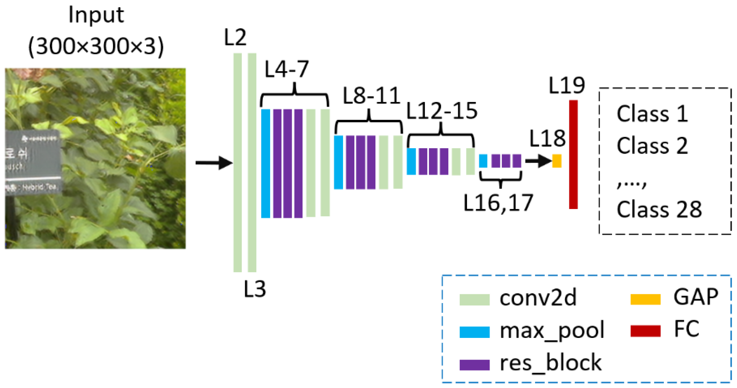
Figure 3.
Structure of the PI-Clas.
Figure 3.
Structure of the PI-Clas.
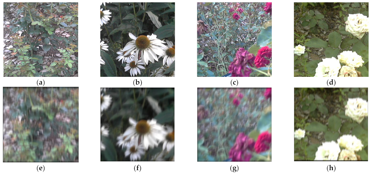
Figure 4.
Sample images of TherVisDb dataset: (a) Alexandra; (b) Echinacea Sunset; (c) Rosenau; (d) White Symphonie; (e–h) corresponding blurry images.
Figure 4.
Sample images of TherVisDb dataset: (a) Alexandra; (b) Echinacea Sunset; (c) Rosenau; (d) White Symphonie; (e–h) corresponding blurry images.
Figure 5.
Accuracy and loss curves of the PI-NMD and PI-Clas: (a) training losses of PI-NMD with an enlarged region in a red box; (b) validation losses of PI-NMD with an enlarged region in a red box; (c) validation and training losses of PI-Clas; (d) validation and training accuracies of PI-Clas.
Figure 5.
Accuracy and loss curves of the PI-NMD and PI-Clas: (a) training losses of PI-NMD with an enlarged region in a red box; (b) validation losses of PI-NMD with an enlarged region in a red box; (c) validation and training losses of PI-Clas; (d) validation and training accuracies of PI-Clas.
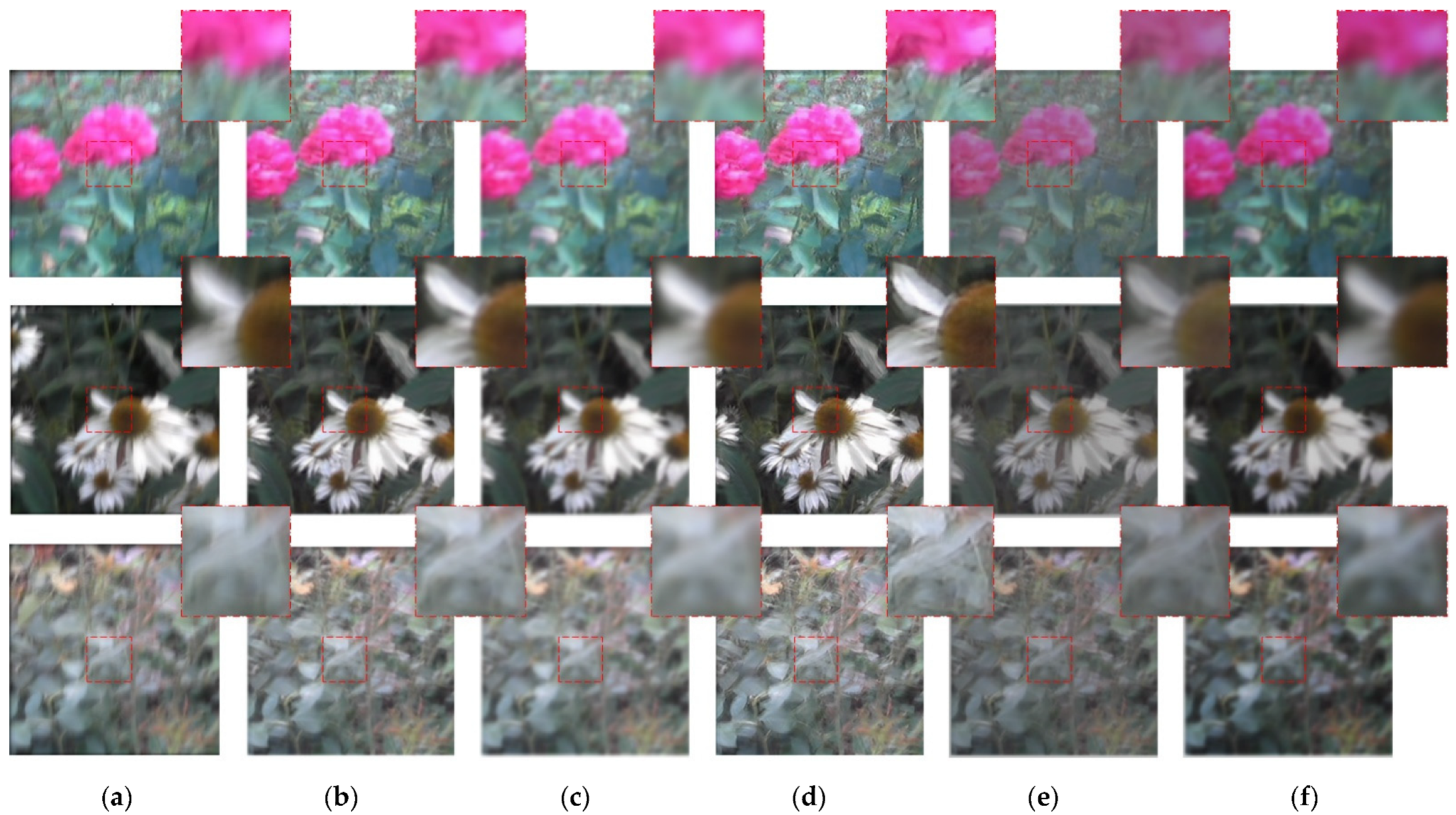
Figure 6.
Examples of images deblurred via PI-NMD. From top to bottom, images of Grand Classe, Echinacea Sunset, and Queen Elizabeth: (a) blurry images; deblurred images generated via (b) Method-1, (c) Method-2, (d) Method-3 (proposed), (e) Method-4, and (f) Method-5.
Figure 6.
Examples of images deblurred via PI-NMD. From top to bottom, images of Grand Classe, Echinacea Sunset, and Queen Elizabeth: (a) blurry images; deblurred images generated via (b) Method-1, (c) Method-2, (d) Method-3 (proposed), (e) Method-4, and (f) Method-5.
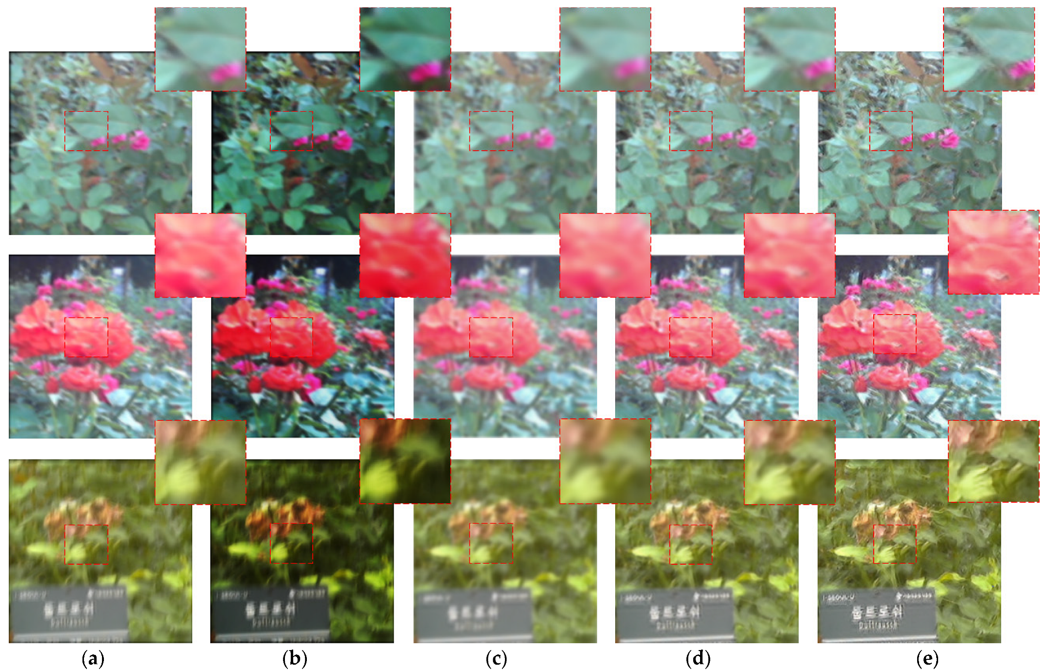
Figure 7.
Example of images deblurred via the PI-NMD and existing deblurring methods. From top to bottom, images of Duftrausch, Grand Classe, and Rose Gaujard. (a) Blurry images and deblurred images via (b) Blind-DeConV, (c) Deblur-NeRF, (d) DeblurGAN, and (e) the proposed PI-NMD.
Figure 7.
Example of images deblurred via the PI-NMD and existing deblurring methods. From top to bottom, images of Duftrausch, Grand Classe, and Rose Gaujard. (a) Blurry images and deblurred images via (b) Blind-DeConV, (c) Deblur-NeRF, (d) DeblurGAN, and (e) the proposed PI-NMD.
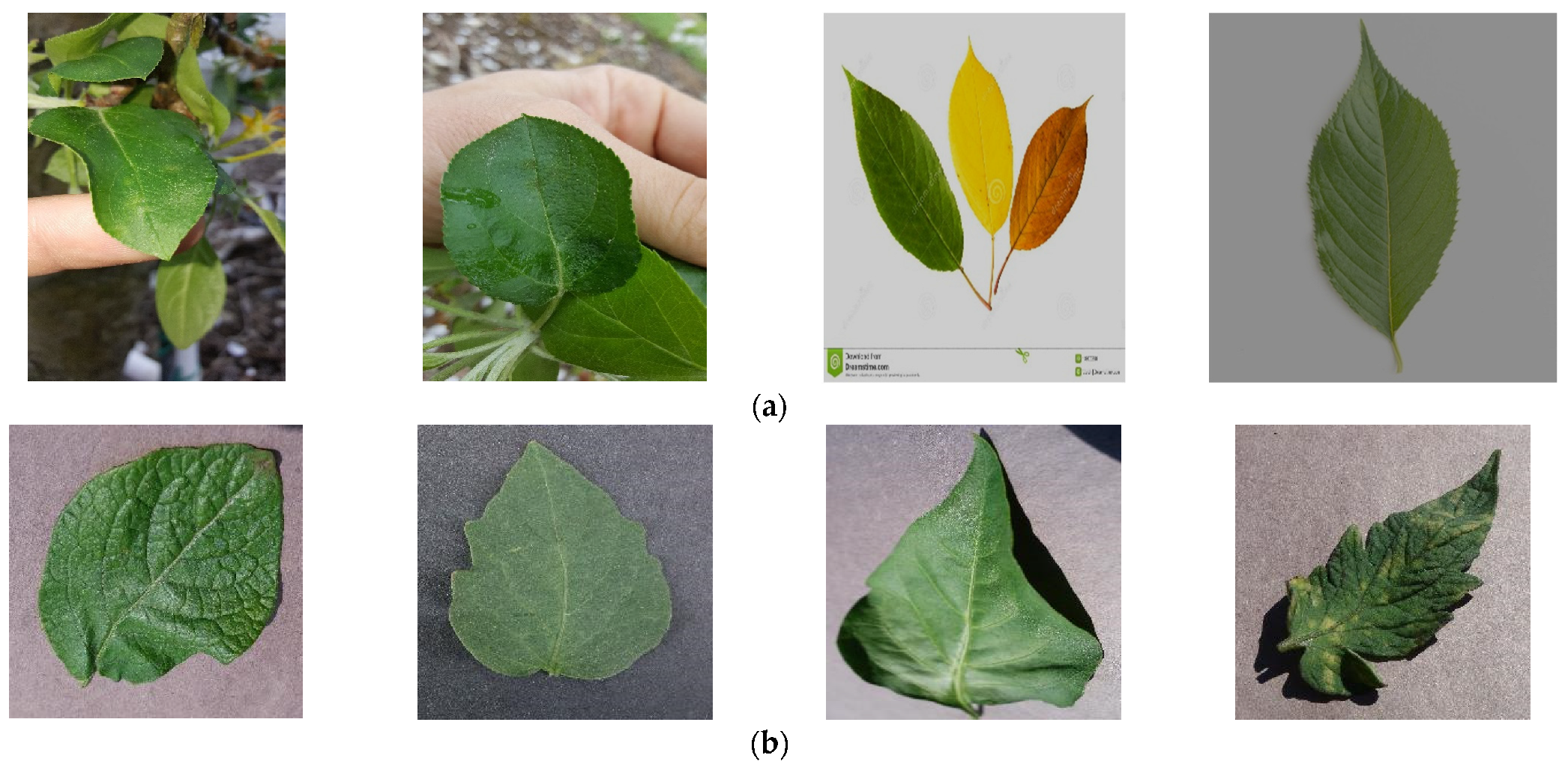
Figure 8.
Sample images of the open datasets: (a) PlantDoc and (b) PlantVillage.
Figure 8.
Sample images of the open datasets: (a) PlantDoc and (b) PlantVillage.
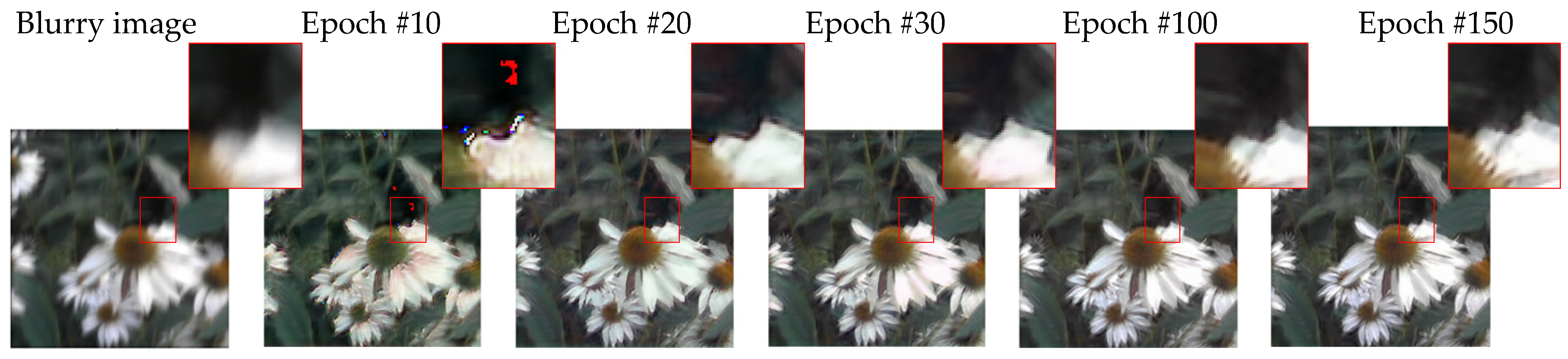
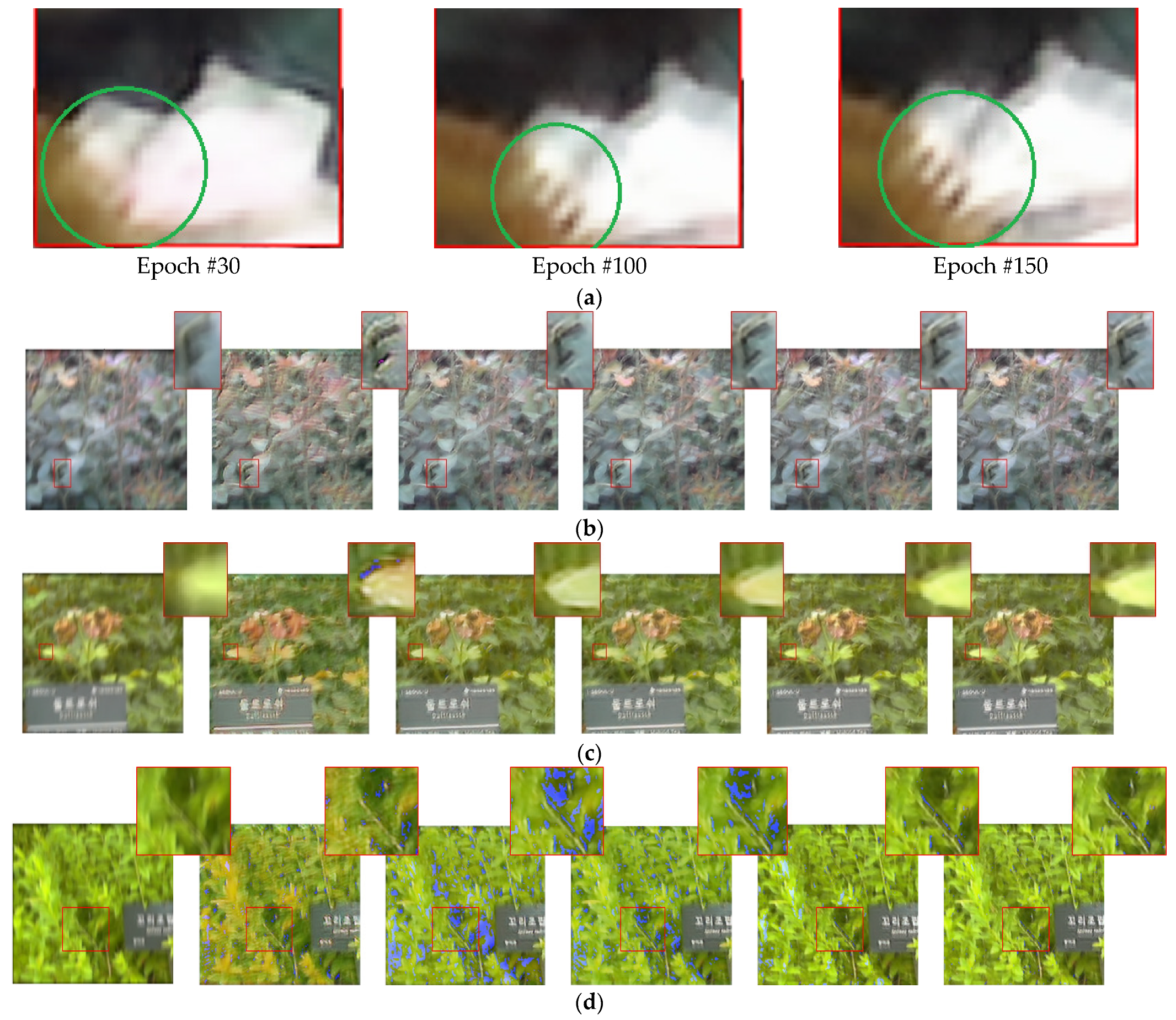
Figure 9.
Examples of error cases: (a) Echinacea Sunset; (b) Queen Elizabeth; (c) Rose Gaujard; (d) Spiraea salicifolia L. From left to right: blurred images; images deblurred at epoch numbers of 10, 20, 30, 100, and 150.
Figure 9.
Examples of error cases: (a) Echinacea Sunset; (b) Queen Elizabeth; (c) Rose Gaujard; (d) Spiraea salicifolia L. From left to right: blurred images; images deblurred at epoch numbers of 10, 20, 30, 100, and 150.
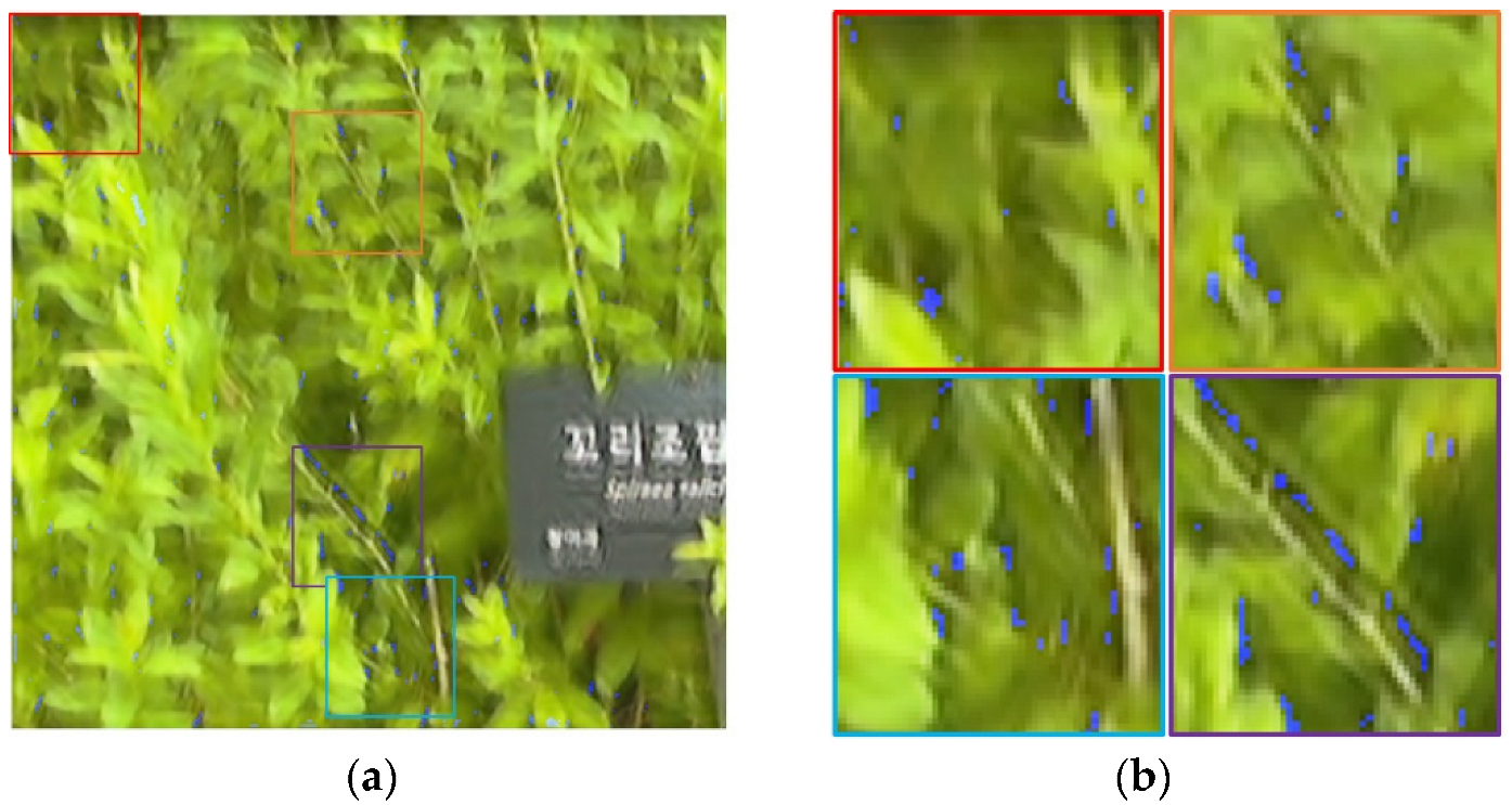
Figure 10.
Examples of the error case: (
a) deblurred image at epoch number 150 (
Figure 9d); (
b) regions enlarged from the image (
a).
Figure 10.
Examples of the error case: (
a) deblurred image at epoch number 150 (
Figure 9d); (
b) regions enlarged from the image (
a).
Figure 11.
Examples of correctly and incorrectly classified images: (
a) Image of Duftrausch correctly classified as Duftrausch image; (
b) image of
Spiraea salicifolia L. (
Figure 10) incorrectly classified as Duftrausch image.
Figure 11.
Examples of correctly and incorrectly classified images: (
a) Image of Duftrausch correctly classified as Duftrausch image; (
b) image of
Spiraea salicifolia L. (
Figure 10) incorrectly classified as Duftrausch image.
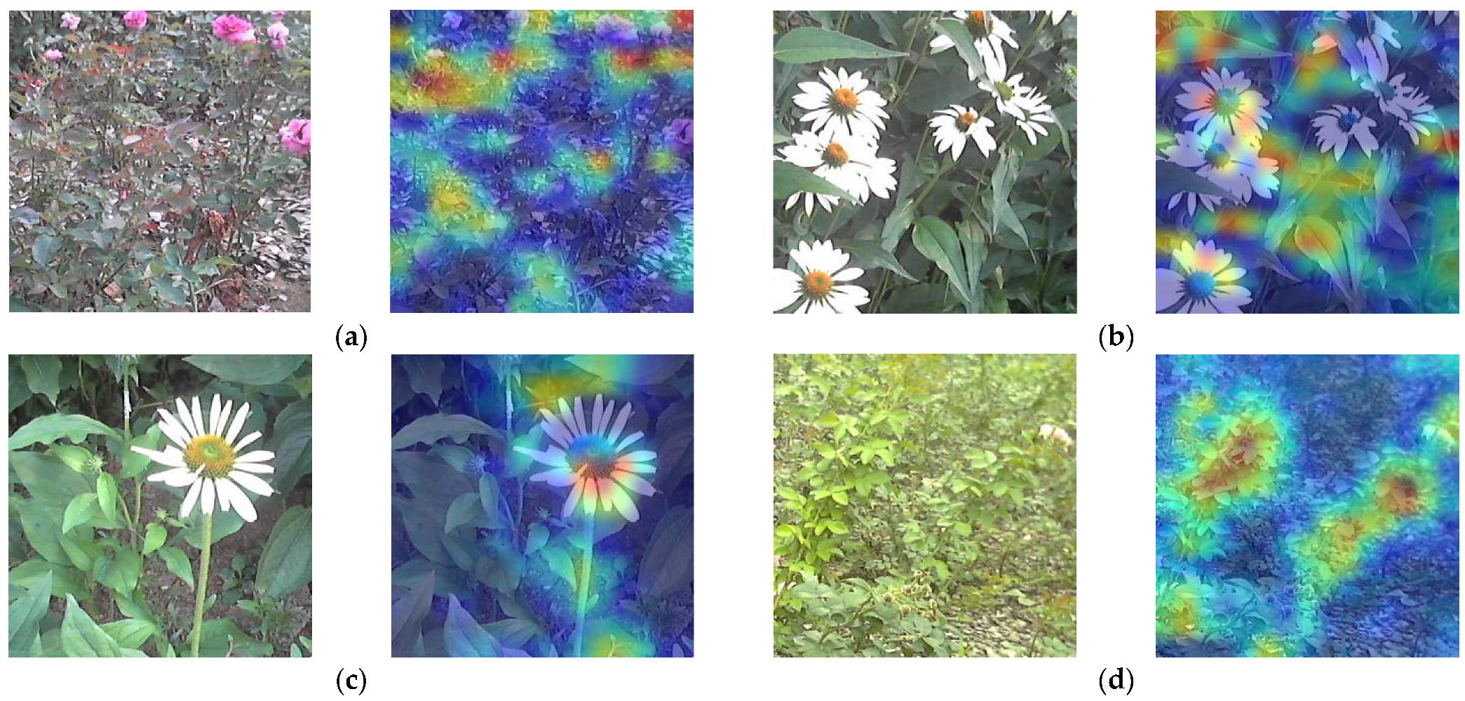
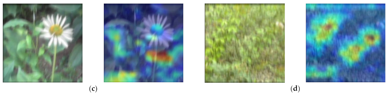
Figure 12.
Example of heatmaps obtained using original images: (a) Blue River; (b,c) Echinacea Sunset; (d) Alexandra.
Figure 12.
Example of heatmaps obtained using original images: (a) Blue River; (b,c) Echinacea Sunset; (d) Alexandra.
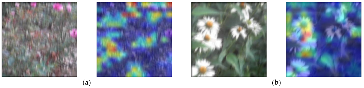
Figure 13.
Example of heatmaps obtained using blurred images: (a) Blue River; (b,c) Echinacea Sunset; (d) Alexandra.
Figure 13.
Example of heatmaps obtained using blurred images: (a) Blue River; (b,c) Echinacea Sunset; (d) Alexandra.
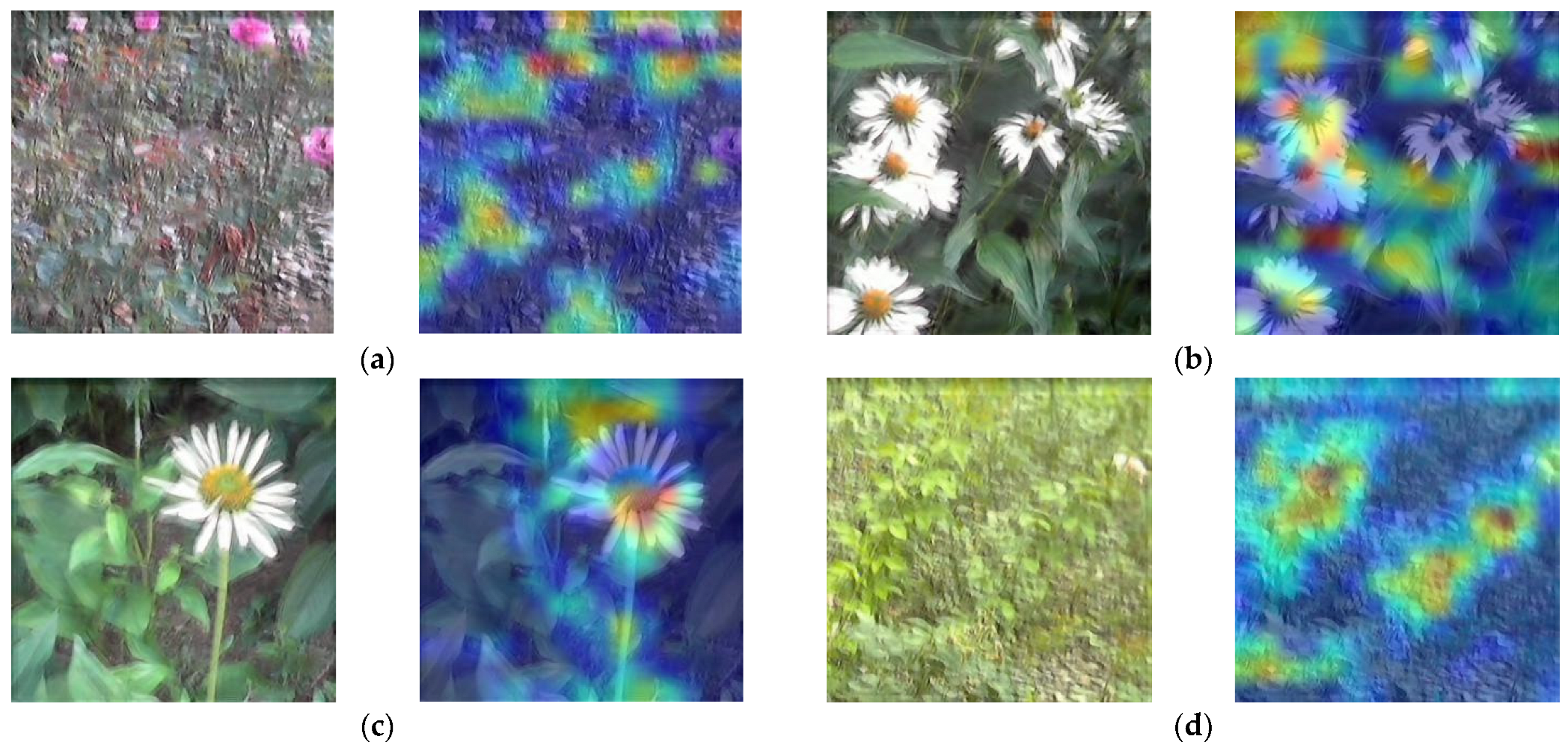
Figure 14.
Example of heatmaps obtained using deblurred images: (a) Blue River; (b,c) Echinacea Sunset; (d) Alexandra.
Figure 14.
Example of heatmaps obtained using deblurred images: (a) Blue River; (b,c) Echinacea Sunset; (d) Alexandra.
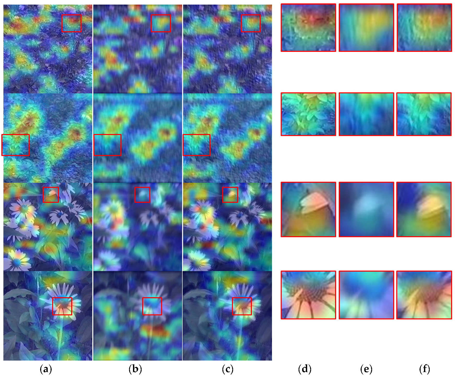
Figure 15.
Comparison of the heatmaps shown in
Figure 12,
Figure 13 and
Figure 14: heatmaps obtained from (
a) original images; (
b) blurred images; (
c) deblurred images. (
d–
f) are the magnified regions of (
a–
c), respectively.
Figure 15.
Comparison of the heatmaps shown in
Figure 12,
Figure 13 and
Figure 14: heatmaps obtained from (
a) original images; (
b) blurred images; (
c) deblurred images. (
d–
f) are the magnified regions of (
a–
c), respectively.
Table 1.
Summary of existing studies on plant image databases.
Table 1.
Summary of existing studies on plant image databases.
| Categories | Methods | Advantages | Disadvantages |
|---|
| Motion deblurring and segmentation | WRA-Net [15] | - -
Provides high-quality (HQ) image; - -
Considers nonlinear motion blur
| - -
Processing time is high; - -
Does not deal with plant image classification
|
| Classification | XGBoost [1], SVMR [2], AAR [3], DenseNet-121 [4], OMNCNN [5], 3-EnsCNNs and 5-EnsCNNs [6], T-CNN [7] | Processing time is low | Do not consider nonlinear motion blur |
| SRR and classification | SRCNN and AlexNet [8], GAN and CNNDiag [9] | Provides HR images | - -
Does not consider nonlinear motion blur; - -
Processing time is high
|
| Nonlinear motion deblurring and classification | PI-NMD and PI-Clas (proposed method) | - -
Provides HQ images; - -
Considers nonlinear motion blur
| Processing time is high |
Table 2.
Description of the generator network of PI-NMD.
Table 2.
Description of the generator network of PI-NMD.
| Layer# | Layer Type | #Filter | Filter Size | Stride Size | Padding Size | Connection |
|---|
| 1 | input_layer | 0 | 0 | 0 | 0 | input |
| 2 | conv2d_1 | 64 | 7 × 7 | 1 | 3 | input layer |
| 3 | conv2d_2 | 128 | 3 × 3 | 2 | 1 | conv2d_1 |
| 4 | conv2d_3 | 128 | 3 × 3 | 2 | 1 | conv2d_2 |
| 5 | res_block × 9 | 128 | 3 × 3 | 1 | 1 | conv2d_3 |
| 6 | Up2_1 | 0 | 0 | 0 | 0 | res_block × 9 |
| 7 | conv2d_4 | 64 | 3 × 3 | 1 | 1 | Up2_1 |
| 8 | Up2_2 | 0 | 0 | 0 | 0 | conv2d_4 |
| 9 | conv2d_5 | 64 | 3 × 3 | 1 | 1 | Up2_2 |
| 10 | conv2d_6 | 3 | 7 × 7 | 1 | 3 | conv2d_5 |
| 11 | add | 0 | 0 | 0 | 0 | conv2d_6 & input_layer |
| 12 | conv2d_7 | 64 | 4 × 4 | 1 | 1 | add |
| 13 | conv2d_8 | 3 | 3 × 3 | 1 | 1 | conv2d_7 |
Total number of parameters: 3,021,638
The number of trainable parameters: 3,017,030
The number of non-trainable parameters: 4608 |
Table 3.
Description of the discriminator network of PI-NMD.
Table 3.
Description of the discriminator network of PI-NMD.
| Layer# | Layer Type | #Filter | Filter Size | Stride Size | Padding Size | Connection |
|---|
| 1 | input_layer | 0 | 0 | 0 | 0 | input |
| 2 | conv2d_1 | 64 | 4 × 4 | 2 | 1 | input_layer |
| 3 | conv2d_2 | 64 | 4 × 4 | 2 | 1 | conv2d_1 |
| 4 | conv2d_3 | 64 | 4 × 4 | 2 | 1 | conv2d_2 |
| 5 | conv2d_4 | 64 | 4 × 4 | 2 | 1 | conv2d_3 |
| 6 | conv2d_5 | 64 | 4 × 4 | 1 | 1 | conv2d_4 |
| 7 | conv2d_6 | 64 | 4 × 4 | 1 | 1 | conv2d_5 |
| 8 | FC | 1 | 0 | 0 | 0 | conv2d_6 |
Total number of parameters: 3,369,601
The number of trainable parameters: 3,369,601
The number of non-trainable parameters: 0 |
Table 4.
Description of the residual block.
Table 4.
Description of the residual block.
| Layer# | Layer Type | #Filter | Filter Size | Stride Size | Padding Size | Connection |
|---|
| 1 | input_layer | 0 | 0 | 0 | 0 | input |
| 2 | conv2d_1 | 128 | 3 × 3 | 1 | 1 | input layer |
| 3 | conv2d_2 | 128 | 3 × 3 | 1 | 1 | conv2d_1 |
| 4 | add | 0 | 0 | 0 | 0 | conv2d_2 & input_layer |
Table 5.
Description of the proposed PI-Clas.
Table 5.
Description of the proposed PI-Clas.
| Layer# | Layer Type | #Filter | Filter Size | Stride Size | Padding Size | Connection |
|---|
| 1 | input_layer | 0 | 0 | 0 | 0 | input |
| 2 | conv2d_1 | 64 | 3 × 3 | 1 | 0 | input_layer |
| 3 | conv2d_2 | 64 | 3 × 3 | 1 | 0 | conv2d_1 |
| 4 | max_pool_1 | 0 | 2 | 0 | 0 | conv2d_2 |
| 5 | res_block × 3 | 64 | 3 × 3 | 1 | 1 | max_pool_1 |
| 6 | conv2d_3 | 128 | 3 × 3 | 1 | 0 | res_block × 3 |
| 7 | conv2d_4 | 128 | 3 × 3 | 1 | 0 | conv2d_3 |
| 8 | max_pool_2 | 0 | 2 | 0 | 0 | conv2d_4 |
| 9 | res_block × 3 | 128 | 3 × 3 | 1 | 1 | max_pool_2 |
| 10 | conv2d_5 | 128 | 3 × 3 | 1 | 0 | res_block × 3 |
| 11 | conv2d_6 | 128 | 3 × 3 | 1 | 0 | conv2d_5 |
| 12 | max_pool_3 | 0 | 2 | 0 | 0 | conv2d_6 |
| 13 | res_block × 3 | 128 | 3 × 3 | 1 | 1 | max_pool_3 |
| 14 | conv2d_7 | 128 | 3 × 3 | 1 | 0 | res_block × 3 |
| 15 | conv2d_8 | 128 | 3 × 3 | 1 | 0 | conv2d_7 |
| 16 | max_pool_4 | 0 | 2 | 0 | 0 | conv2d_8 |
| 17 | res_block × 3 | 128 | 3 × 3 | 1 | 1 | max_pool_4 |
| 18 | GAP | 0 | 0 | 0 | 0 | res_block × 3 |
| 19 | FC | class # | 0 | 0 | 0 | GAP |
| Total number of parameters: 3,733,532 |
Table 6.
Description of the residual block.
Table 6.
Description of the residual block.
| Layer# | Layer Type | #Filter | Filter Size | Stride Size | Padding Size | Connection |
|---|
| 1 | input_layer | 0 | 0 | 0 | 0 | input |
| 2 | conv2d_1 | 64/128 | 3 × 3 | 1 | 1 | input layer |
| 3 | conv2d_2 | 64/128 | 3 × 3 | 1 | 1 | conv2d_1 |
| 4 | add | 0 | 0 | 0 | 0 | conv2d_2 & input_layer |
Table 7.
Description of classes and dataset split.
Table 7.
Description of classes and dataset split.
| Class Index | Class Names | #Image | Set 1 | Set 2 | Validation Set |
|---|
| 1 | Alexandra | 120 | 54 | 54 | 12 |
| 2 | Belvedere | 48 | 21 | 21 | 6 |
| 3 | Blue river | 136 | 61 | 61 | 14 |
| 4 | Charm of paris | 136 | 61 | 61 | 14 |
| 5 | Cleopatra | 152 | 68 | 68 | 16 |
| 6 | Cocktail | 112 | 50 | 50 | 12 |
| 7 | Duftrausch | 176 | 79 | 79 | 18 |
| 8 | Echinacea sunset | 64 | 28 | 28 | 8 |
| 9 | Eleanor | 144 | 64 | 64 | 16 |
| 10 | Elvis | 224 | 100 | 100 | 24 |
| 11 | Fellowship | 208 | 93 | 93 | 22 |
| 12 | Goldeise | 144 | 64 | 64 | 16 |
| 13 | Goldfassade | 184 | 82 | 82 | 20 |
| 14 | Grand classe | 264 | 118 | 118 | 28 |
| 15 | Just joey | 72 | 32 | 32 | 8 |
| 16 | Kerria japonica | 104 | 46 | 46 | 12 |
| 17 | Margaret | 112 | 50 | 50 | 12 |
| 18 | Oklahoma | 312 | 140 | 140 | 32 |
| 19 | Pink perfume | 120 | 54 | 54 | 12 |
| 20 | Queen elizabeth | 120 | 54 | 54 | 12 |
| 21 | Rose gaujard | 312 | 140 | 140 | 32 |
| 22 | Rosenau | 304 | 136 | 136 | 32 |
| 23 | Roseraie du chatelet | 352 | 158 | 158 | 36 |
| 24 | Spiraea salicifolia l | 64 | 28 | 28 | 8 |
| 25 | Stella de oro | 48 | 21 | 21 | 6 |
| 26 | Twist | 288 | 129 | 129 | 30 |
| 27 | Ulrich brunner fils | 120 | 54 | 54 | 12 |
| 28 | White symphonie | 280 | 126 | 126 | 28 |
| Total | 4720 | 2111 | 2111 | 498 |
Table 8.
Comparison of deblurring accuracies via variants of PI-NMD on a blurred image dataset.
Table 8.
Comparison of deblurring accuracies via variants of PI-NMD on a blurred image dataset.
| Methods | #res_block | PSNR | SSIM |
|---|
| Method-1 | 10 | 20.08 | 72.90 |
| Method-2 | 11 | 19.35 | 72.81 |
Method-3
(proposed) | 9 | 21.55 | 73.10 |
| Method-4 | 8 | 18.98 | 72.76 |
| Method-5 | 7 | 18.61 | 72.71 |
Table 9.
Comparison of classification accuracies via variants of PI-Clas on an original HQ image dataset.
Table 9.
Comparison of classification accuracies via variants of PI-Clas on an original HQ image dataset.
| Methods | TPR | PPV | F1 |
|---|
| Method-1 | 84.73 | 89.40 | 87.35 |
| Method-2 | 87.47 | 90.66 | 89.22 |
| Method-3 | 91.12 | 92.33 | 91.71 |
| Method-4 | 92.03 | 92.75 | 92.33 |
| Method-5 | 89.29 | 91.50 | 90.46 |
| Method-6 (proposed) | 93.86 | 93.59 | 93.58 |
Table 10.
Comparison of classification accuracies via variants of PI-Clas on an original HQ image dataset.
Table 10.
Comparison of classification accuracies via variants of PI-Clas on an original HQ image dataset.
| | Top-1 | Top-5 | Top-10 |
|---|
| Method-1 | 84.73 | 95.19 | 97.88 |
| Method-2 | 87.47 | 96.46 | 98.51 |
| Method-3 | 91.12 | 98.15 | 99.36 |
| Method-4 | 92.03 | 98.57 | 99.58 |
| Method-5 | 89.29 | 97.30 | 98.94 |
| Method-6 (proposed) | 93.86 | 99.42 | 100 |
Table 11.
Comparison of classification accuracies via variants of PI-Clas on a blurred image dataset.
Table 11.
Comparison of classification accuracies via variants of PI-Clas on a blurred image dataset.
| Methods | TPR | PPV | F1 |
|---|
| Method-1 | 77.84 | 65.18 | 64.49 |
| Method-2 | 79.14 | 67.00 | 66.97 |
| Method-3 | 80.86 | 69.42 | 70.29 |
| Method-4 | 81.29 | 70.03 | 71.11 |
| Method-5 | 80.00 | 68.21 | 68.63 |
| Method-6 (proposed) | 82.15 | 71.24 | 72.77 |
Table 12.
Comparison of classification accuracies via variants of PI-Clas on a blurred image dataset.
Table 12.
Comparison of classification accuracies via variants of PI-Clas on a blurred image dataset.
| | Top-1 | Top-5 | Top-10 |
|---|
| Method-1 | 77.84 | 85.02 | 91.64 |
| Method-2 | 79.14 | 87.12 | 92.38 |
| Method-3 | 80.86 | 89.92 | 93.38 |
| Method-4 | 81.29 | 90.62 | 93.62 |
| Method-5 | 80.00 | 88.52 | 92.88 |
| Method-6 (proposed) | 82.15 | 92.02 | 94.12 |
Table 13.
Comparison of deblurring accuracies via PI-NMD on variants of the blurred image dataset.
Table 13.
Comparison of deblurring accuracies via PI-NMD on variants of the blurred image dataset.
| PSNR | SSIM |
|---|
| 60/0.01 | 16.34 | 64.81 |
| 60/0.005 | 18.55 | 68.37 |
| 30/0.01 | 20.76 | 72.18 |
| 30/0.005 | 21.55 | 73.10 |
Table 14.
Comparison of classification accuracies via PI-NMD + PI-Clas on blurred datasets blurred with variants of parameters.
Table 14.
Comparison of classification accuracies via PI-NMD + PI-Clas on blurred datasets blurred with variants of parameters.
| TPR | PPV | F1 |
|---|
| 60/0.01 | 83.10 | 87.97 | 91.40 |
| 60/0.005 | 85.80 | 90.24 | 93.75 |
| 30/0.01 | 88.66 | 93.12 | 96.45 |
| 30/0.005 | 90.09 | 78.64 | 84.84 |
Table 15.
Comparison of classification accuracies via PI-NMD + PI-Clas on blurred datasets blurred with variants of parameters.
Table 15.
Comparison of classification accuracies via PI-NMD + PI-Clas on blurred datasets blurred with variants of parameters.
| Top-1 | Top-5 | Top-10 |
|---|
| 60/0.01 | 84.03 | 72.84 | 78.98 |
| 60/0.005 | 86.86 | 75.07 | 81.01 |
| 30/0.01 | 88.97 | 77.47 | 83.36 |
| 30/0.005 | 90.09 | 94.71 | 97.60 |
Table 16.
Comparison of motion deblurring accuracies via the PI-NMD and existing methods.
Table 16.
Comparison of motion deblurring accuracies via the PI-NMD and existing methods.
| Methods | PSNR | SSIM |
|---|
| Blind-DeConV [33] | 17.83 | 67.87 |
| Deblur-NeRF [34] | 20.01 | 72.15 |
| DeblurGAN [22] | 20.89 | 72.41 |
| PI-NMD (proposed) | 21.55 | 73.10 |
Table 17.
Comparison of classification results via existing deblurring methods and PI-Clas.
Table 17.
Comparison of classification results via existing deblurring methods and PI-Clas.
| Methods | TPR | PPV | F1 | Top-5 | Top-10 |
|---|
| Blind-DeConV [33] + PI-Clas | 87.36 | 72.26 | 80.34 | 92.66 | 95.49 |
| Deblur-NeRF [34] + PI-Clas | 88.91 | 76.30 | 82.50 | 93.17 | 96.25 |
| DeblurGAN [22] + PI-Clas | 89.84 | 77.99 | 84.15 | 94.01 | 96.67 |
| PI-NMD + PI-Clas | 90.09 | 78.64 | 84.84 | 94.71 | 97.60 |
Table 18.
Comparison of classification results via existing methods and PI-Clas on the original HQ image dataset.
Table 18.
Comparison of classification results via existing methods and PI-Clas on the original HQ image dataset.
| Methods | TPR | PPV | F1 | Top-5 | Top-10 |
|---|
| AAR network [3] | 91.11 | 88.97 | 89.29 | 98.22 | 100 |
| OMNCNN [5] | 92.21 | 90.82 | 91.80 | 98.51 | 100 |
| T-CNN [7] | 93.03 | 92.20 | 92.69 | 98.71 | 100 |
| AlexNet [8] | 91.08 | 88.53 | 89.12 | 98.18 | 100 |
| CNNDiag [9] | 92.15 | 91.46 | 91.89 | 98.68 | 100 |
| PI-Clas | 93.86 | 93.59 | 93.58 | 99.42 | 100 |
Table 19.
Comparison of classification accuracies via existing methods and PI-Clas on the blurred image dataset.
Table 19.
Comparison of classification accuracies via existing methods and PI-Clas on the blurred image dataset.
| Methods | TPR | PPV | F1 | Top-5 | Top-10 |
|---|
| AAR network [3] | 78.78 | 64.14 | 71.84 | 87.67 | 90.72 |
| OMNCNN [5] | 80.13 | 66.98 | 72.21 | 89.23 | 92.81 |
| T-CNN [7] | 81.14 | 69.11 | 72.49 | 90.74 | 93.48 |
| AlexNet [8] | 78.64 | 63.05 | 71.24 | 87.41 | 90.35 |
| CNNDiag [9] | 81.01 | 67.22 | 72.35 | 90.05 | 93.15 |
| PI-Clas | 82.15 | 71.24 | 72.77 | 92.02 | 94.12 |
Table 20.
Comparison of classification accuracies via existing methods and PI-Clas on the deblurred image dataset via PI-NMD.
Table 20.
Comparison of classification accuracies via existing methods and PI-Clas on the deblurred image dataset via PI-NMD.
| Methods | TPR | PPV | F1 | Top-5 | Top-10 |
|---|
| PI-NMD + AAR network [3] | 85.75 | 70.40 | 78.22 | 90.46 | 94.38 |
| PI-NMD + OMNCNN [5] | 88.09 | 72.87 | 80.53 | 93.00 | 95.83 |
| PI-NMD + T-CNN [7] | 89.08 | 76.88 | 82.62 | 93.45 | 96.60 |
| PI-NMD + AlexNet [8] | 84.85 | 70.38 | 77.98 | 90.10 | 94.18 |
| PI-NMD + CNNDiag [9] | 88.43 | 73.41 | 81.02 | 93.41 | 96.00 |
| PI-NMD + PI-Clas | 90.09 | 78.64 | 84.84 | 94.71 | 97.60 |
Table 21.
Comparison of motion deblurring accuracies via the PI-NMD and existing methods on the open datasets.
Table 21.
Comparison of motion deblurring accuracies via the PI-NMD and existing methods on the open datasets.
| Methods | PlantVillage [14] | PlantDoc [13] |
|---|
| PSNR | SSIM | PSNR | SSIM |
|---|
| Blind-DeConV [33] | 17.46 | 67.02 | 17.56 | 67.43 |
| Deblur-NeRF [34] | 19.50 | 71.40 | 19.18 | 71.37 |
| DeblurGAN [22] | 20.63 | 71.85 | 20.54 | 71.52 |
| PI-NMD | 20.84 | 72.96 | 21.02 | 72.86 |
Table 22.
Comparison of classification accuracies via the PI-Clas on deblurred image datasets via PI-NMD and other methods on the open datasets.
Table 22.
Comparison of classification accuracies via the PI-Clas on deblurred image datasets via PI-NMD and other methods on the open datasets.
| Methods | PlantVillage [14] | PlantDoc [13] |
|---|
| TPR | PPV | F1 | TPR | PPV | F1 |
|---|
| Blind-DeConV [33] + PI-Clas | 86.39 | 71.96 | 80.21 | 79.24 | 64.21 | 71.52 |
| Deblur-NeRF [34] + PI-Clas | 88.21 | 75.80 | 82.48 | 80.78 | 67.60 | 73.98 |
| DeblurGAN [22] + PI-Clas | 89.30 | 77.05 | 83.94 | 81.64 | 69.70 | 75.57 |
| PI-NMD + PI-Clas | 89.79 | 78.48 | 84.00 | 82.21 | 69.78 | 76.52 |
Table 23.
Comparison of classification results via existing methods and PI-Clas on deblurred image datasets via the PI-NMD on the open datasets.
Table 23.
Comparison of classification results via existing methods and PI-Clas on deblurred image datasets via the PI-NMD on the open datasets.
| Methods | PlantVillage [10] | PlantDoc [5] |
|---|
| TPR | PPV | F1 | TPR | PPV | F1 |
|---|
| PI-NMD + AAR network [3] | 85.26 | 69.54 | 77.78 | 77.44 | 61.71 | 69.29 |
| PI-NMD + OMNCNN [5] | 87.46 | 72.24 | 79.74 | 79.59 | 64.57 | 72.06 |
| PI-NMD + T-CNN [7] | 88.30 | 76.30 | 82.54 | 80.54 | 68.25 | 73.85 |
| PI-NMD + AlexNet [8] | 85.10 | 69.21 | 77.13 | 77.12 | 61.15 | 69.02 |
| PI-NMD + CNNDiag [9] | 88.00 | 74.45 | 81.26 | 80.08 | 66.42 | 72.92 |
| PI-NMD + PI-Clas | 89.79 | 78.48 | 84.00 | 82.21 | 69.78 | 76.52 |
Table 24.
Computation time, GFLOPs, number of parameters, model size, and numbers of multiplication and addition per image of each model.
Table 24.
Computation time, GFLOPs, number of parameters, model size, and numbers of multiplication and addition per image of each model.
| Model | Processing Time (ms) | GFLOPs | #Parameters (M) | Model Size (MB) | #Multiplication-Addition
(Giga) |
|---|
| PI-NMD | 55.37 | 49.1 | 3.02 | 12.05 | 49.22 |
| PI-Clas | 51.62 | 40.8 | 3.73 | 44.13 | 40.78 |
| Total | 107.09 | 89.9 | 6.75 | 56.18 | 90.00 |


