Abstract
In the development of a digital twin (DT) for hydropower turbines, dynamic modeling of the system (e.g., penstock, turbine, speed control) is crucial, along with all the necessary data interface, virtualization, and dashboard designs. Since the DT must mimic the actual dynamics of the hydropower turbine accurately, adaptive learning is required to train these dynamic models online so that the models in the DT can effectively follow the representation of the actual hydropower turbine dynamics accurately and reliably. This study presents an adaptive learning method for obtaining the hydropower turbine models for DT development of hydropower systems using the recursive least squares algorithm. To simplify the formulation, the hydropower turbine under consideration was assumed to operate near a fixed operating point, where the system dynamics can be well represented by a set of linear differential equations with constant parameters. In this context, the well-known six-coefficient model for the Francis turbine was formulated as the starting point to obtain input and output models for the turbine. Then, an adaptive learning mechanism was developed to learn model parameters using real-time data from a hydropower turbine testing system. This led to semi-physical modeling, in which first principles and data-driven modeling are integrated to produce dynamic models for DT development. Applications to a pilot system at the Norwegian University of Science and Technology (NTNU) were made, and the models learned adaptively using the data collected from the university’s pilot system. Desired modeling and validation results were obtained.
Keywords:
hydropower systems; Francis turbine; synchronous generator; dynamic modeling; adaptive learning; simulations; MSC:
68Q32
1. Introduction
With an average machine age of more than 64 years, the US hydropower fleet requires smart modernization to reduce costs and enhance the overall reliability and value of the nation’s longest-serving renewable energy technology. Hydropower operations are becoming more complex and demanding as hydropower increasingly provides grid reliability and resiliency while variable renewable energy production, such as solar and wind installations, continues to expand. As the electric power grid prioritizes reliability, resiliency, and value amidst an evolving mix of variable renewable and baseload assets, hydropower technology will require the integration and full benefit of the best available and future advancements in sensors, data and control systems, analytics, simulation, optimization, and computing capabilities to remain competitive. We refer to this need as the hydropower digitalization challenge; the development of a digital twin (DT) would be an effective solution to address such a challenge.
A DT is a combination of a real system and its coupled computational model [1,2,3]. DTs are a hallmark of advanced digitalization within an industry. Data and feedback within a DT provide capacities for autonomy, memory, and embedded intelligence that learn and respond to an evolving environment. This digital embodiment of physical system behavior enables improvements in performance, resource mobilization, asset management, investment planning, and scenario analysis. DT adoption has grown rapidly since its inception in 2003 to address needs for design, production, prognostics, and health management [4,5]. DTs are used to design new products in a responsive, efficient, and informed manner, and to synchronize design and production. DTs are also used to monitor, control, and optimize production processes reliably and flexibly—DT-enabled production optimization has reduced material waste and prolonged machine lifetime [3,4,5,6,7,8,9,10]. However, DT market penetration is limited [6,7,8,9]; fewer than 15% of industries use DTs, and the rest have nascent or no plans to implement DTs in the next 5 years. DT development in the electric power sector, including hydropower, is nascent [10] but has been embraced by and benefited manufacturing. For example, the Turlough Hill hydroelectric plant in Ireland uses a DT to implement predictive maintenance, thereby improving reliability and reducing costs for an aging facility, but DT applications for hydropower systems are few [11].
In this context, Figure 1 shows the basic components of a DT for hydropower systems—an open platform framework, as described in [12]. It can be seen that the framework will collect data from real hydropower systems and continuously update its dynamic models for various components of hydropower systems. Thus, the DT can comprehensively represent the actual plant operation in digital form for use in operational optimization, condition monitoring, and workforce training. The framework also has a powerful user interface, including visualization and augmented reality, to allow user-friendly functionalities for the hydropower industry, hydropower system equipment manufacturers, and academia.
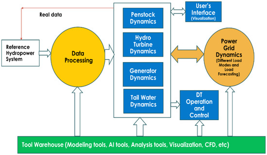
Figure 1.
Structure of a DT for hydropower systems.
Based on the described framework and requirements, in the development of a DT for hydropower systems, dynamic modeling of the system (such as the penstock, turbine, generator, and linkages to the power grid units) is important, in addition to all the necessary data interface, virtualization, and dashboard designs. Since the DT must mimic the actual dynamics of the hydropower system accurately, adaptive learning is required to train the dynamic models online so that the models in the DT can effectively and responsively follow the representation of the actual hydropower system dynamics accurately and reliably. This effectiveness requires the integration of physical modeling with data-driven approaches to enable the models in the DT to learn and update their parameters in real time when new sets of data are collected from the reference hydropower systems, as shown in Figure 1. In this context, adaptive learning methods such as the recursive least squares method [12,13] should be used together with the structure of the physical models [14,15] to learn the dynamics of the system. Indeed, parameter estimation and system identification have been used for hydropower systems for some time [16,17,18,19]. For example, a system identification method for estimating the relationship between the water level and generating power was developed in [16]. System identification has also been used to estimate the transfer functions of hydropower dynamics for frequency containment reserves [17]. For nonlinear feature estimation, in [18], a neural network-based method has been developed for the predictive control of hydropower plant operational efficiency. In this context, an adaptive fuzzy particle swarm optimization approach has been used to estimate parameters of the hydro-turbine regulation system [19].
In this work, we present an adaptive learning method to obtain the online models for hydropower turbines in the DT development of hydropower systems, as shown in Figure 1. We emphasize the establishment of adaptive modeling of water flow and turbine speed control systems. To simplify the formulation, we assumed that the system under consideration operates near a fixed operating point, where the system dynamics can be well represented by a set of linear differential equations with constant parameters [20]. In this context, the well-known six-coefficient model [21] for the Francis turbine was formulated as a starting point in the state space form. Once these state space physical models were established, a set of input and output models [13] were obtained, and an adaptive learning mechanism was developed to update input and output model parameters in real time using the data from the hydropower system [16]. This leads to semi-physical modeling, in which first principles and data-driven modeling are effectively integrated to produce dynamic turbine models. In comparison with the existing methods, the linearized six-coefficient models formulated in this paper define the correct model structure and number of parameters to be estimated using an online scheme, while data-driven modeling and learning are performed using the simple yet well-known recursive least squares algorithm. Such a combination provides a fast adaptive learning solution for online modeling and learning that is effective for the learning phase of the digital twin when it is connected to the actual hydropower plant. Applications to a pilot testing system in the Water Power Laboratory at the Norwegian University of Science and Technology (NTNU) were made, and the models were learned adaptively using the data collected from the test system with desired modeling and validation results.
The rest of the paper is organized as follows: Section 2 describes the formulation of the six-coefficient model for the Francis turbine in the state space form together with standard discretization. Section 3 describes the establishment of transfer function-based input and output models so that the hydropower turbine could be modeled by a set of transfer functions. Section 4 presents an adaptive learning algorithm using the recursive least squares learning principle in which the model parameters can be learned and updated using real-time data. Section 5 describes applications to the testing hydropower system at NTNU, showing the effectiveness of the proposed adaptive learning strategy. Section 6 presents conclusions and future work. The nomenclature is defined in Table 1.

Table 1.
Nomenclature.
2. Turbine System Model
The water system for realizing electricity generation should consider the features of the reservoir, penstock, turbine chamber, and discharge (tail water stream), all of which together comprise a complex nonlinear hydropower dynamic system that requires data-driven modeling and initial manufacturing data from turbine manufacturers. By using hydropower turbine-generator experimental data, we can construct a systematic model for simulating the hydropower generator system for DT development.
As shown in Figure 2, the operational system for hydropower turbine units consists of the penstock dynamics, turbine, speed sensor, speed controller, and a hydraulic servo that amplifies the control output to drive the guide vane opening for the control of the water flow to the turbine, where the transfer function reveals the relationship between the net torque and the shaft speed with being the Laplace variable.
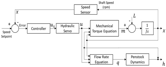
Figure 2.
Control flow of the hydropower turbine control system.
2.1. Turbine Speed (Frequency) Control System
The control structure of the turbine speed is shown in Figure 2; the closed-loop system consists of the dynamics of the turbine, hydraulic servo, and controller. For the hydropower turbine to be controlled, the input is the guide vane opening that controls the amount of water entering the turbine, and the output is the shaft speed (frequency) and the water head. The objective of such a closed-loop control is to maintain the required shaft speed (frequency) subjected to load changes, as denoted by , when the hydropower generation is connected to the power grid and, at the same time, minimize the water head variations.
2.2. Torque and Water Flow Module
Figure 2 also shows the torque and water flow rate modules when the generation unit operates. In the hydropower turbine dynamics for the mechanical torque and water flow rate, the inputs are the guide vane opening, the shaft speed, and the water head, respectively. The outputs are the turbine torque () and water flow rate ().
The following nonlinear functions are generally used:
where is the time-varying variable denoting the turbine speed (rad/s), which is related to the frequency through with being the turbine-generator frequency controlled around 50 Hz for the NTNU testing system when the hydropower generation unit is connected to the grid. In Equation (1), is the water head, and is the guide vane opening. are two unknown nonlinear functions that need to be learned using the operational real-time data from the actual plant.
Throughout this paper it is assumed that the turbine operates at a selected fixed operating point, , for the hydropower generation unit connected to the grid. Based on the fixed operating point , the relative (normalized) incremental values of turbine shaft speed, water head, water flow rate, guide vane opening, and torque are defined as follows.
where is the normalized incremental value for the shaft speed, is the normalized incremental water head, is the normalized incremental water flow rate, is the normalized incremental guide vane opening, and is the normalized incremental mechanical torque, with being the turbine operating torque that maintains the operating point . Since , , , m, and are all normalized incremental variables, they do not have physical units. In this context, the initial boundary conditions for the variables in Equation (2) are all set to zero, as in the modeling it is assumed that the system has the operating point as initial boundary conditions.
Using definitions in Equation (3), the nonlinear dynamics of the mechanical torque and water flow rate can be linearized to provide the following six-coefficient linearized dynamic model for the normalized incremental torque () and the normalized incremental water flow rate () of the turbine [21].
where , , and are the linearized coefficients for the torque generation calculated at a fixed operating point . , , and are the linearized coefficients for the water flow rate calculated at a fixed operating point . These six coefficients [21] are obtained from
These constants can be estimated based on experimental data. Using these definitions, the shaft rotation can be expressed by the following dynamics (i.e., the swing equation):
where is a load torque in normalized incremental sense and , with being the inertia.
2.3. State Space Model for Non-Elasticity Water System Dynamics
When the water in the penstock is incompressible, the system is regarded as nonelastic [22,23]. In this case, the relationship between the water head and the water flow rate is
In Equation (5), the input is the normalized incremental water flow rate (), and the output is the normalized incremental water head (), as defined in Equation (3), and is the water inertia time constant, which is defined as
where is the length of penstock pipeline, and and are from the operating point . For the NTNU testing system used in this study, 0.0415 m2·s. By integrating the linearized Equations (3)–(9) into a state space format, the following state space model can be readily obtained.
where , , , and are formulated using the six-coefficient linearized models in Equations (3)–(5) to give:
In the system, the input is the normalized incremental value of the guide vane opening and its rate of change, and the outputs are the shaft speed and the water head. Figure 3 shows such a state space model structure.
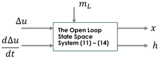
Figure 3.
Open-loop system structure.
The open-loop stability of the hydropower turbine can be ensured if all the eigenvalues of are inside the left-hand side of the complex plane. The turbine torque is used to balance the grid load, which can be generally expressed as
where is the damping ratio contributed by the power grid, and is the load, which is assumed here to be less than 10% of total load variations since large load changes would trigger the nonlinearities of the mechanical torque and water flow rate and make the linearized model unsuitable.
2.4. State Space Model for Elastic Water Flows
Again, for linearized modeling, nonelastic water flow was considered for large water head and long penstock. In this case, the following better approximated water system dynamics are used [23]:
This transfer function shows the second order dynamics between the water heads and the water flow rate. In Equation (10),
where is the wave travel time, “” is the Laplace variable, and = 1480 m/s is the velocity of the sound travelling in the water.
Thus, the following time-domain differential equation can be formulated, which links the water flow rate to the water head in the normalized incremental sense as defined in Equation (3) for the hydropower turbine.
In this case, the state vector for the penstock dynamics is denoted as
Then, the following penstock state space model can be obtained:
where is regarded as a kind of calculable input to the penstock system for elastic water flows. Further formulation of Equation (18) using the six-coefficient model and Equation (8) leads to:
Combining these two equations gives
At this stage, the extended state vector is denoted as
Then, the following state space model of the whole turbine dynamics for the elastic water flow can be obtained:
In this case, the state space form can be represented as
where system matrices in Equation (8) become
This format indicates that the system has third-order dynamics—again subjected to the inputs of the normalized incremental values of the guide vane opening and its rate of change, as shown in Figure 3.
These open-loop state space models can be further transferred into direct input and output models that help construct the adaptive learning algorithms that use available collected real-time data to learn the component models of the hydropower turbine and estimate relevant model parameters.
2.5. PID Controller for Shaft Speed
The open-loop system structure shown in Figure 3 can be integrated with the controller (speed governor) to form a typical closed-loop control system for the shaft speed, as shown in Figure 2. In this context, the controller should be designed so that the shaft speed is well controlled within its targeted set point ranges with minimal variation in the water head, and it should be subjected to the operational constraint on the rate of changes for the guide vane opening as well. In this context, the widely used PID controller has the following form [23]:
where is the tracking error of the normalized incremental shaft speed, is the output of the controller (i.e., the output of the speed governor of the hydropower turbine as shown in Figure 2), is the proportional gain, is the integral gain, is the derivative gain, and is the time. The selection of these control gains was determined from the test rig at NTNU during the test runs. In the real-time control set-up, the above PID controller is discretized in line with the following discretization procedure in the next subsection, where the PID control is represented as a second-order linear time-constant differential equation.
2.6. Discretization
The control design objective is to obtain the speed control signal, the governor’s output , so that optimally tracks zero with a required bounded rate of changes. Considering that the system in either Equation (12) or Equation (26) is linear time-invariant, this study uses the discretization equations as follows:
where is the sampling time interval for the discretization. By applying this discretization to the state space models, the discretized model can be obtained. For the NTNU test rig, 0.2 s, indicating that there are five sampled points per second.
2.7. Hydraulic Servo for the Guide Vane Opening
The output of the speed controller will normally be amplified by a hydraulic servo system that has enough power to operate the movement of the guide vane. The guide vane opening is denoted as .
In general, the hydraulic servo in the waterpower laboratory at NTNU can be modeled in a discretized format as second-order dynamics at sampling interval s.
where is the output of the hydraulic servo, which is also the guide vane opening, and is the output of the speed controller as shown in Figure 2.
3. Discretized Input and Output Models
To facilitate the estimation of the system parameters, the following transfer function models will be formulated using the state space model in Equations (12) and (26).
The objective was to obtain the relationship between the input (guide vane opening) and the outputs (the shaft speed and the water head). For this purpose, these input and output models were formulated in the Laplace transformation domain. Moreover, nonelastic and elastic water flows were both considered.
3.1. Input and Output Model for Nonelastic Water Flow
When the system is under nonelastic water flow with a constant load (, in the Laplace transform format, the following equations reveal the relationship between the shaft speed and the water head with respect to the guide vane opening.
where “” in Equations (38) and (39) denotes the Laplace variable.
Also, to simplify the representation, when variables such as are used together with the Laplace variable “s”, they are inherently in their Laplace transformed senses.
By solving the water head from Equation (39), the following can be obtained:
By substituting Equation (40) into Equation (38) and rearranging all the terms, the following can be obtained:
Thus, the relationship between and for nonelastic water flow is given as
where it has been denoted that
Accordingly, the transfer function between and is
To summarize, we have
Equations (46) and (47) reveal how the guide vane opening affects the shaft speed and water head during system operation under nonelastic water flow. In the next subsection, similar models for elastic water flow are formulated.
3.2. Input and Output Model for Elastic Water Flow
In cases where the water is compressible, simple second-order dynamics, as shown in Equation (16), can be used. Using this elastic water model for penstock, a similar formulation to Equations (38)–(47) can also be performed to obtain the input and output models for the guide vane opening, shaft speed, and water head. For example, Equation (38) stays the same, and the water head and flow rate dynamics become:
Re-arranging Equation (48) leads to the following model:
which reveals the relationship of the water head with respect to the speed and the guide vane opening as the control input.
Substituting Equation (49) into Equation (38) and eliminating leads to the following direct relationship between the shaft speed and the guide vane opening:
where it can be formulated that
which are third-order and second-order polynomials, respectively. As in general , the denominator in Equation (51) satisfies the necessary condition for the stability for the speed system.
Equation (50) shows that the dynamics between the shaft speed and guide vane opening follow a third-order differential equation when the water flow is elastic.
4. Least Squares Adaptive Learning Scheme Using Real-Time Data for Elastic Water Flows Case
Using the models developed in Section 3, relevant learning strategies can be obtained for estimating the input and output model parameters using the sampled data from the actual system. In this context, only the system with elastic water flow was examined since the nonelastic water flow has simpler equations for describing the dynamics among the guide vane opening, shaft speed, and water head.
Equation (50) shows that the system has third-order elastic water flow between the guide vane opening and the shaft speed. In this context, the discretization using Equation (32) would lead to the following discretized input and output model between the shaft speed and the guide vane opening [13].
where and are the sampled shaft speed and guide vane opening of the turbine in their normalized incremental senses, respectively. is the sampling index, is the sampling period as denoted before, and is related to the discretized and normalized incremental value of the load torque, with being a coefficient. , , , , , and are the coefficients to calibrate.
Assuming that the data are collected from the test runs in which the load is constant, then in most cases, and the estimation of is not necessary. Furthermore, are coefficients as a result of discretization, and they are complicated functions of the six coefficients defined in Equations (6) and (7) and other parameters in the state space model represented in Equations (24) and (25).
Assuming that the real-time data can be collected and denoted as the data sequence of , then the objective of parameter learning for the input and output model is to use these collected input and output data to estimate the model parameters in Equation (53). Of course, once these parameters are well estimated, the original six coefficients inside the state space model can be formulated using the inverse mapping between model parameters in Equation (53) and the six coefficients in the state space model. For this purpose, we denote:
Then, when the test runs for the data collection are under a fixed load condition, Equation (53) can be simply expressed by
Assuming that the current sample time is and the data are available from up to , the least squares algorithm can simply be used to recursively estimate the parameters as shown in the following form:
where is the estimate of at sample time , and is a variance matrix calculated from Equation (59). The initial values of (k) and are prespecified depending on prior knowledge of the parameter values. The structure of adaptive learning is shown in Figure 4, which is in line with the generic learning scheme in [24,25].
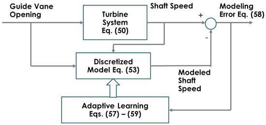
Figure 4.
Adaptive learning of parameters θ for elastic water flow.
Equations (57)–(59) constitute a learning strategy to estimate model parameters and ultimately the six coefficients. Once the parameters are estimated, they would constitute adaptive modeling for the hydropower turbine.
In the same way, the model for water head can also be learned adaptively. Equation (18) shows that the discretized model of the water head is of the following form:
Therefore, Equation (60) can be further expressed in the following vector form—Equation (61)—which is similar to that in Equation (56):
Thus, the similar recursive least squares algorithm to that in Equations (57)–(59) can be modified to estimate , where the adaptive learning structure is again similar to that in Figure 4.
5. Experimental and Data Processing
This section describes the hydropower experimental data collection at NTNU and the process for estimating the model parameters in Section 4. For this purpose, a hydropower system control experiment was conducted, and the data were collected by collaborators at NTNU. The system structure is shown in Figure 5, where the water head ranged from 12 to 30 m and the flow rate ranged from 0.1 to 0.4 m3/s during testing and data collection.
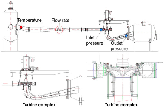
Figure 5.
Structure of the hydropower generator system.
The main variables measured and collected were the shaft speed, flow rate, pressure difference (i.e., water head) between inlet and outlet pressures, guide vane opening, mechanical torque, and load torque. The goal of processing the experimental data was to obtain the normalized values for these variables and ensure that they were uniformly sampled for the discretization models. The variables are summarized in Table 2. Six measurements of these variables were collected in the experiment in the waterpower laboratory at NTNU. Since the sampling interval for these variables was from different sensors, the sample frequency and total sample size from the sensors varied significantly. For example, the samples collected for the differential pressure were around 506 per 0.1 s, whereas the samples collected for the turbine speed were 4–7 per one second. Therefore, to consistently use the data, preprocessing was needed to clean up unnecessary information from the experimental data and unify the data sampling frequency to 5 Hz; this means that there are five sampled points per second with , which was then used for discretized models in Equations (53) and (60).
Table 2.
Experimental data summary.
Six groups of tests were conducted with changes in experiment conditions at the test rig at NTNU in June and July 2022. First, four open-loop tests (Tests 1–4) were conducted in which the guide vane opening () was directly changed while keeping other initial conditions fixed; the system load was fixed at 378 N·m, and the power generated was 14.9 kW. In this experiment, the maximum guide vane opening angle was 14°.
In Test 1, the guide vane opening went from 6.63° to 7.63°; in Test 2, it went from 7.60° to 6.60°; in Test 3, it went from 6.60° to 5.60°; in Test 4, it went from 5.60° to 6.60°. These changes reflect the open-loop tests in which the input was the guide vane opening and the outputs were the other variables in Table 2. In addition to the open-loop tests, two closed-loop tests (Tests 5 and 6) were conducted. Test 5 was carried out by changing the shaft speed set point from 342 to 360 rpm with speed control PI gains at = 7.5 and = 0.5. Test 6 was carried out by changing the shaft speed set point from 360 to 342 rpm at = 7.5 and = 0.15. The recursive least squares method in Equations (57)–(59) was used to learn the system parameters grouped in given by Equation (54), and the estimated outputs of the shaft speed, water head, and water flow rate were calculated using the estimated model parameters and compared with the actual system response data. The sampling frequency of turbine shaft speed (rpm) was used as a reference for unifying the data collection frequency. Therefore, the sample data were collected approximately every 0.2 s. For the measurements with sampling frequencies different from the sampling frequency of the turbine shaft speed (rpm), the value of the sample at the same time as the turbine shaft speed (rpm) sample was obtained through interpolation.
Also, all the responses of shaft speed, guide vane opening, water flow, and water head were in the normalized incremental sense as defined in Equation (3) except the shaft speed in the following figures, which are the true values. The operating point in the test runs was selected as follows:
In the test runs, the magnitudes of perturbations of the guide vane opening for the open-loop tests and the set point of the shaft speed were less than ±1° and ±18 rpm, respectively. These values are of sufficiently small magnitudes to ensure that the assumption of linearization is satisfied. With such small magnitudes of input changes, the formulation of the models in Section 2, Section 3 and Section 4 is valid in representing the linearized dynamics of the system.
5.1. Learning of Input and Output Models for Elastic Case
During learning, the first two open-loop testing data sets were combined in the data preprocessing stage. Figure 6 shows the responses of the six variables in a normalized incremental sense, where the light-green curve is the guide-vane opening, the read curve stands for the torque, the light-blue line displays the shaft speed, the split red line around zero is the water flow, and the blue curve describes the water pressure.
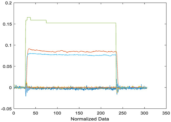
Figure 6.
Data of normalized incremental responses of shaft speed, water flow rate, water head, torque, and guide vane opening collected for Tests 1 and 2.
In applying the adaptive learning algorithm in Equations (57)–(59), the initial and the variance matrix were selected, with being the 5 × 5 identity matrix.
Figure 7 shows the two responses of the shaft speed in the top diagram; the blue line represents the original actual speed response , and the red line represents the estimated shaft speed (k) in the progress of the adaptive learning using the recursive least squares algorithm in Equations (57)–(59). This has clearly demonstrated the desired adaptive learning effect, as these two variables are very close to each other. In this case, the estimated shaft speed was calculated from the following model.
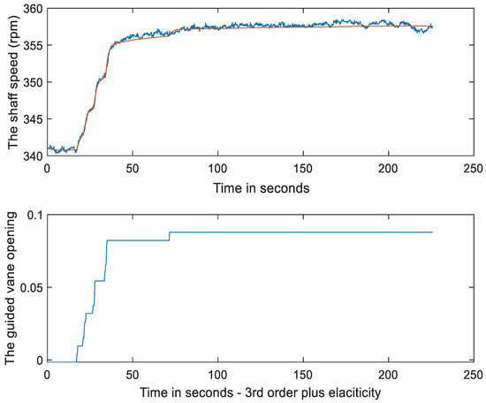
Figure 7.
Shaft speed in rmp, its estimated value , and the guide vane opening in its normalized incremental value.
Equation (37) shows the learned model, and the modeling error for the shaft speed is thus defined as
This modeling error is different from the residual signal in the adaptive learning algorithm Equations (57)–(59) because is different in the two equations. The model uses the same guide vane opening as presented in Figure 4. In Figure 7, the bottom diagram provides the actual system input—the guide vane opening in its normalized incremental values.
Figure 8 shows the modeling error reflected by the calculation in Equation (64) when the adaptive learning phase in Equations (57)–(59) is progressing. As shown in Figure 8, the modeling error was less than 1% in general. The maximum absolute modeling error was 0.84%. On the other hand, for the water head, the learned model is given by
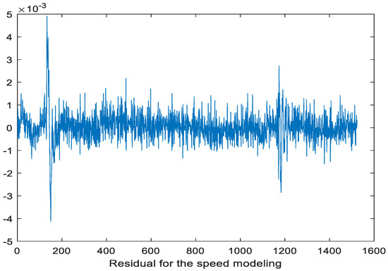
Figure 8.
Response of the shaft speed modeling error when the adaptive learning Equations (57)–(59) is progressing for Tests 1 and 2.
Accordingly, Figure 9 and Figure 10 show the responses of the actual and estimated water flow rate and water head, with the blue-colored curve as the real data and the red-colored curve as the model outputs. The figures confirm that the desired learning effect was obtained.
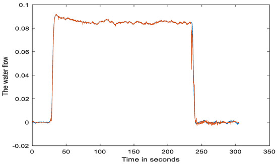
Figure 9.
Actual and estimated water flow rates in normalized incremental values.
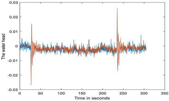
Figure 10.
Actual and estimated water heads in normalized incremental values.
At the end of the run for Tests 1 and 2, the estimated has the following value:
Therefore, since for Tests 1 and 2, the discretized model for the shaft speed and the guide vane open is given by
Similarly, after the test runs and adaptive learning application, the estimated parameters for the water head model are given by , which indicates that the model for the water head is
Since the water starting constant is at a constant 0.0415 in the NTNU test rig, Equation (67) becomes
For Test 5, the actual system responses are shown in Figure 11, all in the normalized incremental sense.
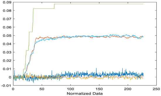
Figure 11.
Actual system responses of shaft speed, water flow rate, pressure, guide vane opening, and torque all in the normalized incremental sense as in Equation (3).
Again, using the adaptive learning algorithm in Equations (57) and (59), the estimated values of the shaft speed, water flow rate, and pressure were obtained. The estimated variables were calculated using Equation (66), which resulted in the responses in Figure 12, Figure 13 and Figure 14.

Figure 12.
Top: actual and estimated shaft speeds in rpm. Bottom: actual guide vane opening in its normalized incremental values in the closed loop shaft speed control mode.
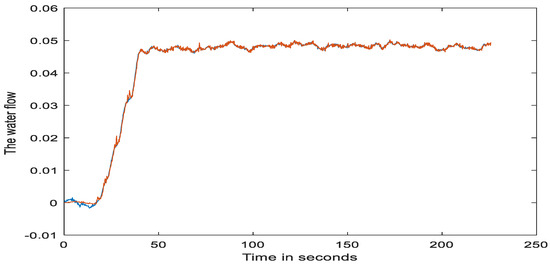
Figure 13.
Actual and estimated water flow rate in the normalized incremental values. The blue line stands for real data and the red line for the model output.
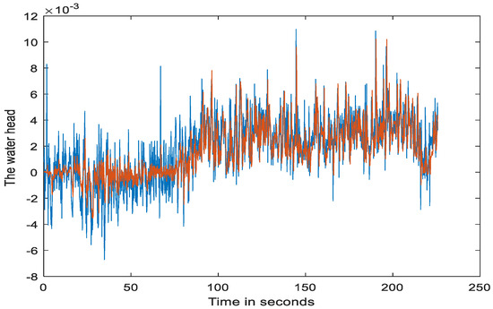
Figure 14.
Actual (blue) and estimated (red) water heads in their normalized incremental values.
Again, all the actual and estimated system responses were very close to each other, demonstrating the desired learning and estimation effects. These responses can be regarded as a side-by-side simulation when the DT is linked in parallel to the actual hydropower turbine unit in a synchronous manner. In this case, the DT must generate synchronized, close-to-actual system responses to ensure that it can accurately learn the dynamics of the system.
5.2. Direct Estimate of the Six Coefficients
Since for the NTNU hydropower testing rig the mechanical torque and the water flow rate can be directly measured together with the shaft speed, water head, and guide vane opening, we can also use Equations (4) and (5) to obtain the least squares estimate of the six coefficients [21] at the operating point defined by
In this context, the matrix form of the least squares method for calculating these six coefficients through the batched data is shown as follows:
where is the column of the normalized incremental values of the turbine speed, is the column of the normalized incremental values of the water head, is the column of the normalized incremental values of the guide vane opening, is the column of the normalized incremental values of the turbine mechanical torque, and, finally, is the column of the normalized values of the water flow rate.
Thus, for test runs 1 and 2, the six-coefficient {, , , , , } is estimated using Equations (69) and (70) to be {−0.1438, 0.1513, 0.1178, −0.0222, 0.0646, 0.0026}.
6. Conclusions
In this study, an adaptive learning model was developed for hydropower turbines using the recursive least squares approach as the learning strategy for the initial development of a DT for hydropower systems. Under the assumption that the system operates near a fixed operating point defined by the shaft speed, water flow rate, water head, and guide vane opening, a set of linearized models was formulated in the state space and input and output forms using six-coefficient modeling in hydropower turbine modeling. Recursive least squares learning was then established to estimate the model parameters of the input and output models for the shaft speed and water head. The desired modeling results were obtained through a set of experiments on a Francis turbine in the Waterpower Laboratory test rig at NTNU. The model outputs closely tracked the actual system outputs effectively, with very small tracking errors, demonstrating the potential of using the developed adaptive learning for DT development in the near future. Moreover, since the NTNU test rig can directly measure the mechanical torque and water flow rate, a direct estimation of the six coefficients was also made using the least squares algorithm.
The work reported here focused on adaptive learning models for hydropower turbines alone for digital twin development. Future efforts will be needed to include a synchronous generator in the modeling so that adaptive learning modeling for the whole hydropower generating unit can be obtained. In addition, considering the large variation in dynamics, nonlinear system modeling using integrated physical modeling and data-driven approaches (such as neural networks [24,25]) is also needed to capture the nonlinearities of the system.
It can be seen that once the digital twin is established, as shown in Figure 1, it can be used to generate comprehensive operational scenarios for the operators to optimize the plant operation. It can also simulate and generate faulty scenario data that can be used to validate various fault diagnosis and prediction strategies, making it a key tool for predictive maintenance in the hydropower industry.
Author Contributions
Conceptualization, H.W.; methodology, H.W.; software, S.O.; validation, H.W. and S.O.; formal analysis, H.W. and S.O.; investigation, H.W. and S.O.; resources, P.-T.S., O.G.D., H.I.S. and I.V.; data curation, P.-T.S. and O.G.D.; writing—original draft preparation, H.W. and S.O.; writing—review and editing, H.W. and S.O.; visualization, H.W. and S.O.; supervision, H.W.; project administration, H.W.; funding acquisition, H.W. All authors have read and agreed to the published version of the manuscript.
Funding
The work reported here is funded by the US Department of Energy’s Water Power Technologies Office with the grant titled “Digital Twin for Hydropower Systems—an Open Platform Framework” under Contract DE AC05 76RL01830.
Data Availability Statement
The data used to generate the results belong to the project use only and cannot therefore be made available to the public.
Acknowledgments
This work was also supported by the resources at the National Transportation Research Center at Oak Ridge National Laboratory (a User Facility of DOE’s Office of Energy Efficiency and Renewable Energy), and is in line with the MOU between the U.S. Department of Energy (DOE) and Norway’s Royal Ministry of Petroleum and Energy to collaborate on hydropower research and development. In the project phase, we have also received suggestions and comments from DoE technical managers, Colin Sasthav and Kyle Desomber. These are gratefully acknowledged.
This manuscript has been authored by UT-Battelle, LLC, under contract DE-AC05-00OR22725 with the US Department of Energy (DOE). The US government retains and the publisher, by accepting the article for publication, acknowledges that the US government retains a nonexclusive, paid-up, irrevocable, worldwide license to publish or reproduce the published form of this manuscript, or allow others to do so, for US government purposes. DOE will provide public access to these results of federally sponsored research in accordance with the DOE Public Access Plan (http://energy.gov/downloads/doepublic-access-plan (accessed on 20 August 2023).
Conflicts of Interest
The authors declare no conflict of interest.
References
- ARUP. Digital Twin: Towards a Meaningful Framework; ARUP: London, UK, 2019. [Google Scholar]
- Parrott, A.; Warshaw, L. Industry 4.0 and the Digital Twin: Manufacturing Meets Its Match; Deloitte: Olathe, KS, USA, 2017. [Google Scholar]
- Tao, F.; Zhang, H.; Liu, A.; Nee, A.Y.C. Digital Twin in Industry: State-of-the-Art. IEEE Trans. Ind. Inform. 2019, 15, 2405–2415. [Google Scholar] [CrossRef]
- Vachálek, J.; Bartalský, L.; Rovný, O.; Šišmišová, D.; Morháč, M.; Lokšík, M. The digital twin of an industrial production line within the industry 4.0 concept. In Proceedings of the 2017 21st International Conference on Process Control (PC), Štrbské Pleso, Slovakia, 6–9 June 2017; pp. 258–262. [Google Scholar]
- Knapp, G.L.; Mukherjee, T.; Zuback, J.S.; Wei, H.L.; Palmer, T.A.; De, A.; DebRoy, T. Building blocks for a digital twin of additive manufacturing. Acta Mater. 2017, 135, 390–399. [Google Scholar] [CrossRef]
- Costello, K.; Omale, G. Gartner Survey Reveals Digital Twins Are Entering Mainstream Use. Available online: https://www.gartner.com/en/newsroom/press-releases/2019-02-20-gartner-survey-reveals-digital-twins-are-entering-mai (accessed on 13 October 2022).
- Goasduff, L. Confront Key Challenges to Boost Digital Twin Success. Available online: https://www.gartner.com/smarterwithgartner/confront-key-challenges-to-boost-digital-twin-success (accessed on 13 October 2022).
- Kosan, L. Digital Twin Technology: Where Are We Now? Available online: https://www.iotworldtoday.com/2019/05/08/digital-twin-technology-where-are-we-now/ (accessed on 13 October 2022).
- Martynova, O. Digital Twin Technology: A Guide for Innovative Technology. Available online: https://intellias.com/digital-twin-technology-guide/ (accessed on 13 October 2022).
- Lund, A.M.; Mochel, K.; Lin, J.-W.; Onetto, R.; Srinivasan, J.; Gregg, P.; Bergman, J.E.; Hartling, K.D.; Ahmed, J.A.; Chotai, S. Digital Wind Farm System. US Patent No. US20160333855A1, 17 November 2016. [Google Scholar]
- Water Power Technologies Office. Water Power Technologies Office Releases First Multi-Year Program Plan; Water Power Technologies Office: Washington, DC, USA, 2022.
- Wang, H.; Ahmed, O.; Smith, B.T.; Bellgraph, B. Developing a digital twin for hydropower systems—An open platform framework. Int. Water Power Dam Constr. Mag. 2021, 81, 24–25. [Google Scholar]
- Wang, H.; Liu, Y.Q.; You, D.H. Application of a Nonlinear Self-tuning Controller for Regulating the Speed of a Hydraulic Turbine. J. Dyn. Syst. Meas. Control 1991, 113, 541–544. [Google Scholar] [CrossRef]
- Giosio, D.R.; Henderson, A.D.; Walker, J.M.; Brandner, P.A. Physics-Based Hydraulic Turbine Model for System Dynamic Studies. IEEE Trans. Power Syst. 2017, 32, 1161–1168. [Google Scholar] [CrossRef]
- Pennacchi, P.; Chatterton, S.; Vania, A. Modeling of the dynamic response of a Francis turbine. Mech. Syst. Signal Process. 2012, 29, 107–119. [Google Scholar] [CrossRef]
- Gracino, R.; Hansen, V.; Goia, L.; Campo, A.; Campos, B. System Identification of a Small Hydropower Plant. In Proceedings of the 2021 14th IEEE International Conference on Industry Applications (INDUSCON), São Paulo, Brazil, 15–18 August 2021; pp. 1430–1434. [Google Scholar]
- Jakobsen, S.H.; Bombois, X.; Uhlen, K. Non-intrusive identification of hydro power plants’ dynamics using control system measurements. Int. J. Electr. Power Energy Syst. 2020, 122, 106180. [Google Scholar] [CrossRef]
- Adedayo, O.O.; Gbadamosi, S.L.; Ale, D.T. Neural Network Predictive Controller for Improved Operational Efficiency of Shiroro Hydropower Plant. Int. J. Sci. Eng. Res. 2015, 6, 1454–1459. [Google Scholar]
- Liu, D.; Xiao, Z.; Li, H.; Liu, D.; Hu, X.; Malik, O.P. Accurate Parameter Estimation of a Hydro-Turbine Regulation System Using Adaptive Fuzzy Particle Swarm Optimization. Energies 2019, 12, 3903. [Google Scholar] [CrossRef]
- Zeng, Y.; Zhang, L.X.; Qian, J.; Guo, Y.K.; Xu, T.M. Additional Mechanical Torque Coefficients of Hydro Turbine and Governor System. Adv. Mater. Res. 2012, 443–444, 954–961. [Google Scholar] [CrossRef]
- Li, H.; Chen, D.; Zhang, H.; Wang, F.; Ba, D. Nonlinear modeling and dynamic analysis of a hydro-turbine governing system in the process of sudden load increase transient. Mech. Syst. Signal Process. 2016, 80, 414–428. [Google Scholar] [CrossRef]
- Fang, H.; Shen, Z. Modeling and Simulation of Hydraulic Transients for Hydropower Plants. In Proceedings of the 2005 IEEE/PES Transmission & Distribution Conference & Exposition: Asia and Pacific, Dalian, China, 18 August 2005; pp. 1–4. [Google Scholar]
- Yang, W. Hydropower Plants and Power Systems: Dynamic Processes and Control for Stable and Efficient Operation. Doctoral Dissertation, Electricity, Department of Engineering Sciences, Technology, Disciplinary Domain of Science and Technology, Uppsala University, Uppsala, Sweden, 2017. [Google Scholar]
- Mu, C.; Wang, K.; Ni, Z. Adaptive learning and sampled-control for nonlinear game system using dynamic event-triggering strategy. IEEE Trans. Neural Netw. Learn. Syst. 2022, 33, 4437–4450. [Google Scholar] [CrossRef] [PubMed]
- Wang, Q.; Psillakis, H.E.; Sun, C.; Lewis, F.L. Adaptive NN distributed control for time-varying networks of nonlinear agents with antagonistic interactions. IEEE Trans. Neural Netw. Learn. Syst. 2021, 32, 2573–2583. [Google Scholar] [CrossRef] [PubMed]
Disclaimer/Publisher’s Note: The statements, opinions and data contained in all publications are solely those of the individual author(s) and contributor(s) and not of MDPI and/or the editor(s). MDPI and/or the editor(s) disclaim responsibility for any injury to people or property resulting from any ideas, methods, instructions or products referred to in the content. |
© 2023 by the authors. Licensee MDPI, Basel, Switzerland. This article is an open access article distributed under the terms and conditions of the Creative Commons Attribution (CC BY) license (https://creativecommons.org/licenses/by/4.0/).