Project Group Program Generation and Decision Making Method Integrating Coupling Network and Hesitant Fuzzy

Abstract

Modern urban construction relies on a large number of projects. Project groups are an effective way to manage a large number of projects. In view of the current lack of scientific methods for constructing and evaluating project group programs, which are mainly based on subjective experience, this article proposes a scientific method for project group program generation and decision-making. The method proposed in this article applies a multi-layer coupling network to the modeling of project groups and divides projects into planning projects and execution projects to form a heterogeneous coupling network. Then, starting from the principle of project information dissemination, the evaluation indicators of the project group program were defined, and finally, the hesitant fuzzy decision-making method was used to assist in decision making. This article can provide a new method for project group construction and management, and provide strong support for the construction of smart cities and digital governments.

1. Introduction

In the current era of rapid economic development, how the government can quickly carry out urban construction and development is an important topic of this era. The current urban construction and management are transforming towards digitalization and intelligence, and the corresponding urban construction and development methods are also improving in this direction [1]. Currently, various types of engineering projects are the main means for the government to carry out urban construction. Therefore, using scientific and digital means to carry out and manage projects is an important part of realizing the construction of smart cities and digital governments [2].

A project is the basic organizational form of current major engineering construction. It refers to activities carried out to achieve a specific purpose, obtain a certain result, and integrate various resources to solve a certain problem. With the improvement of productivity and the increase in construction demand in various fields, the number of projects being approved has increased significantly. In order to facilitate the management of a large number of projects, the concept of the program was proposed. All projects in the project group serve the core goals of the project group. Due to the long implementation period and large resource consumption, such goals are broken down into more detailed goals and requirements, and each project assumes the corresponding part.

In project groups, since projects are often closely connected, project risks are often spread due to project-undertaking relationships, resulting in the entire project group being unable to achieve the expected goals. The failure of large-scale project groups will also bring immeasurable losses to society, cause serious emergencies, and threaten the development process of society. Therefore, effective management of the project group will be related to the success of the entire project program. In order to manage the project group, an effective project group management method must be proposed. Project group management plays an important role in the construction of smart cities and digital governments. It can help organize and coordinate multiple related projects and ensure synergy between projects to achieve the goals of smart cities and digital government. Through project group management, the overall planning and management efficiency of the project can be improved, and the development of smart cities and digital governments can be promoted.

There is currently sufficient research on individual project management, but there is a lack of research on project group management. In the management of a large number of projects and project groups, the following two problems still exist: Firstly, the management of project groups still lacks reasonable theoretical methods, and the relationship allocation of projects within the project group still relies mainly on experience. Secondly, there is a lack of understanding of project groups in overall evaluation systems and methods.

Therefore, the research questions of this article are mainly as follows:

• How are project groups modeled and represented? There are multiple projects in the project group, and the project types and project attributes are different. Which method should be used to reasonably describe the project group and be displayed using mathematical means?
• The management of project groups still lacks reasonable theoretical methods, and the relationship allocation of projects within the project group still relies mainly on experience.
• There is a lack of understanding of project groups in overall evaluation systems and methods.

Aiming at the above problems, this paper carried out the modeling and evaluation research of the program group. The novel works studied in this paper are mainly as follows:

• The structure of the project group was analyzed, based on which a Planning Execution Network (PEN) was proposed. A multi-layer coupling network is used to model the PEN, and a mathematical model of the project group is obtained.
• Starting from the mechanism of information interaction, the logic of project group management is analyzed. Based on this, two indicators, management performance and execution performance, are proposed as standards for evaluating project group programs.
• The hesitant fuzzy decision-making method is combined with the problem background of project group program evaluation to provide theoretical scientific assistance for the selection and decision-making of project group programs.

2. Related Works

2.1. Project and Project Group Management

Project management is a complex discipline including team building, time arrangement, planning process, project cost estimation, project interface management, risk management, avoiding potential risks to accomplish project goals, and other stages [3]. Modern project management can be traced back to around World War II. The Gantt chart, invented by Henry L. Gantt in the 1930s, is considered an early tool and method for project management. After that, Critical Path Method (CPM) [4,5], Program Evaluation and Review Technique (PERT) [6,7], Graphic Evaluation and Review Technique (GERT) [8,9], Work Breakdown Structure (WBS) [10,11,12] and Earned Value Management (EVM) [13,14,15] methods in the field of project management were born.

In recent years, the research on project management has made new progress and methods. Reusch [16] extends project management processes according to PMBOK to improve project management and project control. A new knowledge area for sustainability management in projects is introduced with a base set of new processes. Loehr [17] extends the PMI standards on project management and defines processes for project finance management. The literature [18] focuses on the extension of project procurement concepts and processes with the aim of integrating sustainable procurement into the project management methodology provided by the PMBOK framework. Boonstra [19] examines how project complexity influences the choice of a project management strategy and presents a framework that facilitates managers in selecting a suitable project management strategy. The work by Wu et al. [20] is based on the project portfolio management technology to introduce a new energy projects management system.

Project group management refers to the overall control and coordination of multiple projects on the basis of individual project management to achieve the organization’s strategic goals and benefits [21]. According to the International Project Management Association (IPMA), “Project group management is the coordination and management of multiple projects with the aim of enabling barrier-free communication between projects to achieve a set of business objectives” [22]. The concept of the current project group was only proposed recently. Although project group management has great potential in managing multiple projects at the same time, its application is not very widespread. The Philips Petroleum Company built a large number of service stations in the United States to seek sales for products that increase production. This is a relatively successful case of the implementation of project group management ideas [23]. In addition, leading electronic product manufacturing companies such as IBM, HP, and Northern Telecom also recognize the effectiveness of project group management, which can be used to improve the quality, efficiency, and reliability of products and services, and shorten product development time [24].

Keller [25] predicts the performance of project groups in R & D organizations. Chevrier [26] aims at better understanding the dynamics of international project groups by grasping the strategies project leaders set up to cope with cultural diversity. Gevers et al. [27] addresses this issue that many project groups have a hard time meeting their deadlines.

2.2. Coupling Network

Multi-layer networks use layers to highlight the differences in nodes and connections between different levels. A coupling network refers to a network composed of nodes at different levels generating shared connections to achieve coupling. Since coupling networks are suitable for describing the internal operating mechanisms of complex systems, there has been much research on the mechanisms and characteristics of coupling networks in recent years. Murata [28] conducted an in-depth study of the coupling mechanism of coupling networks, proposed a generalization method for inter-layer coupling in multi-layer networks, and tried to use it to detect communities in multi-layer networks. The literature [29] studies the impact of inter-layer coupling on the centrality measurement of multi-layer networks, and discusses the effects of two popular inter-layer coupling methods: diagonal coupling and diagonal coupling with cross-coupling between adjacent layers. The literature [30] studies the synchronization of multi-layer fully coupled networks and their simplest equivalent networks, and discusses the important factors affecting synchronization. In terms of application, it is often used to explore issues such as information dissemination and material dissemination, and is used in fields such as public health, transportation, and public opinion monitoring. The specific application research is shown in

Table 1. Summary of coupling network applications.

Research Problem	Field of Application	Research Content	Literature
Information dissemination	Public opinion monitoring	The propagation law of the public opinion coupled double-layer network is studied	[31]
		Focuses on coupling mechanism of online public opinion events	[32]
		Research on the spread speed of public opinion	[33]
	Rumors spread	Study the principle of rumor spreading with reference to the rumor spreading mechanism of infectious diseases	[34]
		Rumor diffusion mechanism in coupling network	[35]
		The law of opinion dissemination and evolution of individual opinions	[36]
	Social contagion	Social contagion dynamics of non-redundant information memory	[37]
		credit risk contagion	[38]
Material transmission	Transportation	Learn the multi-aspect traffic data couplings	[39]
	Energy transmission	Study the scenario of multi-energy complementary system accessing medium-voltage distribution network	[40]
		Provides the constraints of network balance and system energy security	[41]
	Public health	Numerical identification of prevalence thresholds for the susceptibility-infection-recovery model on finite-sized networks	[42]
		Properties of epidemic thresholds for susceptibility-infection-susceptibility dynamics in networks	[43]
		Threshold of epidemic spread in the network	[44]
		Velocity and Hierarchical Spread of Outbreaks in Scale-Free Networks	[45]
		Susceptible infection transmission dynamics with adjustable power-law response time distributions	[46]
		Contagion processes on the static and activity-driven coupling networks	[47]
	Ecosystem	species migration spread	[48]

. Therefore, due to the coupling network’s better explanation and restoration of the information propagation mechanism and its similarity to the tree structure of the project group organization, this article decided to use the coupling network to model and describe the project group organization plan.

2.3. Fuzzy Decision Theory

In decision theory, in order to more appropriately represent the situation that is difficult to discretely determine in decision-making, the concept of fuzzy mathematics has been introduced into decision theory by academic circles. In 1965, Zadeh [49] proposed the concept of fuzzy sets for the first time. In 2009, Spanish scholar Torra [50] proposed the concept of hesitant fuzzy sets. In 2011, Xu Zeshui [51] formally gave the mathematical expression of hesitant fuzzy sets, and then the concept of hesitant fuzzy has been widely used in decision-making problems in various fields. Ref. [52] utilizes binary connection number theory to obtain the hesitant fuzzy center and decision-making suggestions about the alternative ranking under different hesitant fuzzy conditions. Ref. [53] proposed a hesitant fuzzy hypergraph model based on hesitant fuzzy sets and fuzzy hypergraphs. Ref. [54] defines a new kind of hesitant fuzzy set, namely the time-sequential hesitant fuzzy set, to perfect the description of such hesitant situations and obtain more reasonable results of decision making.

In terms of application, decision-making theory based on hesitant fuzzy theory is widely used in social [55], political [56], economic [55,57] and other fields. Qian et al. [58] apply hesitant fuzzy theory to a decision support system. Liu [59] presents a new representation of the hesitant fuzzy linguistic term sets by means of a fuzzy envelope to carry out the computing with words processes. Liao [60] shows the efficiency of the proposed correlation coefficients; they are implemented in medical diagnosis and cluster analysis.

2.4. Literature Summary

In summary, the existing coupling network theory effectively describes the mechanism of information transmission in some social application scenarios and conducts modeling analysis; hesitant fuzzy decision-making theory is also applied to important program decisions for social construction and people’s livelihood.

However, the above-mentioned research still has many shortcomings. There are many research contents on project management, but there are few studies on forming a large number of projects into project groups. The theory of coupled networks is often used in fields such as energy, health, and public safety, but it is rarely used in project management and program management. In addition, research on combining methods such as project management, coupled network modeling, and hesitant fuzzy methods is still lacking.

This paper combines the characteristics of the project group decision-making problem with a strong structure, many participants, and high decision-making risks, and describes the project group structure based on the transmission of accusation information through the coupling network. On this basis, it evaluates the capability efficacy of the projects in the project group network using the hesitant fuzzy decision-making method to rank the overall execution capabilities based on the effectiveness of the capabilities, thereby achieving decision support.

3. Preliminaries

3.1. Hesitation Fuzzy Theory

Assuming a fixed set X, a hesitant set X is a function that maps each element to a subset of [0, 1]. The mathematical expression for the hesitant fuzzy set is [51]:

$$A=\{<x,h_A\left(x\right)>|x\in X\}$$

(1)

where $h_A\left(x\right)$ is the set of some values in [0, 1] representing some possible degrees of affiliation of the element x with respect to the set A. $h=h_A\left(x\right)$ is called a hesitant fuzzy element, and $\mathsf{\Theta }$ is used to represent the set of all hesitant fuzzy elements [61].

For fuzzy element h, its score $s\left(h\right)$ is [51]:

$$s\left(h\right)=\frac{1}{l_h}\sum _{\gamma \in h}\gamma$$

(2)

where $l_h$ is the number of elements in h and $\gamma$ is the elements in the set h.

Then, the deviation degree $\overline{\sigma }\left(h\right)$ of h is [51]:

$$\overline{\sigma }\left(h\right)={\left[\frac{1}{l_h}\sum _{\gamma \in h}{(\gamma -s(h\left)\right)}^2\right]}^{\frac{1}{2}}$$

(3)

where $s\left(h\right)$ is defined similarly to the mean in statistics, $\overline{\sigma }\left(h\right)$ is similarly to the standard deviation, reflecting the degree of deviation of all the values in the hesitant fuzzy element h from their mean.

Let $h_1$ and $h_2$ be two hesitant fuzzy elements, $s\left(h_1\right)$ and $s\left(h_2\right)$ be the result of $h_1$ and $h_2$ score; $\overline{\sigma }\left(h_1\right)$ and $\overline{\sigma }\left(h_2\right)$ are the deviations of $h_1$ and $h_2$, respectively. $h_1$ is better than $h_2$; it is recorded as $h_1>h_2$. $h_1$ and $h_2$ has no difference; it is recorded as $h_1\sim h_2$. Then, the hesitant and fuzzy sorting method is [62]:

If $s\left(h_1\right)<s\left(h_2\right)$, then $h_1<h_2$;

If $s\left(h_1\right)=s\left(h_2\right)$, then:

• If $\overline{\sigma }\left(h_1\right)=\overline{\sigma }\left(h_2\right)$, then $h_1\sim h_2$,
• If $\overline{\sigma }\left(h_1\right)<\overline{\sigma }\left(h_2\right)$, then $h_1<h_2$,
• If $\overline{\sigma }\left(h_1\right)>\overline{\sigma }\left(h_2\right)$, then $h_1>h_2$.

Suppose $A=\{h_1,h_2,\cdots ,h_n\}$ is a n dimensional hesitant fuzzy element set, and denote $\theta$ as the integration function defined on the set of hesitant fuzzy elements, $\theta :{[0,1]}^n\to [0,1]$, then [63]:

$${\theta }_A=\bigcup _{\gamma \in \{h_1\times h_2\times \cdots \times h_n\}}\left\{\theta \right(\gamma \left)\right\}$$

(4)

This paper uses the Hesitant Fuzzy Weighted Average (HFWA) operator, which is a mapping ${\mathsf{\Theta }}^n\to \mathsf{\Theta }$, whose form is [63]:

$$HFWA(h_1,h_2,\cdots ,h_n)=\underset{i=1}{\overset{n}{\oplus }}{w}_i{h}_i=\bigcup _{{\gamma }_1\in h_1,{\gamma }_2\in h_2,\cdots ,{\gamma }_n\in h_n}\left\{1-\prod _{i=1}^n{(1-{\gamma }_i)}^{w_i}\right\}$$

(5)

where $w={(w_1,w_2,\cdots ,w_n)}^T$ is the weight vector of $h_i(i=1,2,\cdots ,n)$, $w_i\in [0,1]$, $i=1,2,\cdots ,n$, and ${\displaystyle \sum _{i=1}^n}{w}_i=1$.

In particular, if the weights are equal, i.e., $w={(\frac{1}{n},\frac{1}{n},\cdots ,\frac{1}{n})}^T$, then the HFWA operator degenerates into a hesitant fuzzy average (HFA) operator [63]:

$$HFA(h_1,h_2,\cdots ,h_n)=\frac{1}{n}\underset{i=1}{\overset{n}{\oplus }}{h}_i=\bigcup _{{\gamma }_1\in h_1,{\gamma }_2\in h_2,\cdots ,{\gamma }_n\in h_n}\left\{1-\prod _{i=1}^n{(1-{\gamma }_i)}^{\frac{1}{n}}\right\}$$

(6)

3.2. Planning Execution Network (PEN)

We define two types of projects within a project group: planning projects and execution projects.

Planning project: The planning project is the project responsible for resource scheduling and schedule management of other projects. Achieve the ultimate goal of the planning project through other projects.

Execution project: The execution project carries out the actual main business, which is responsible for participating in various research, construction and business activities, and forming a supporting role for the planning project.

The internal organization of the program depends on the connection between different projects. The connection between projects represents the jurisdiction support relationship between different projects and also includes the transmission of project information. The set of all projects is $P=\{p_1,p_2,\cdots ,p_m\}$, and the formed jurisdiction relationship constitutes the edge set of the network $E=\{e_1,e_2,\cdots ,e_s\}$, so the Planning-Execution Network (PEN) is obtained $G= <P,E>$.

The project group network is divided into two types of projects, planning projects and execution projects. Planning projects are recorded as $p^a$, and their collections are recorded as $P^a$; various execution projects are recorded as $p^b$, and its set is recorded as $P^b$. The distribution of the two types of programs is as follows:

$$P=\{\underset{P^a}{\underbrace{p_1,\cdots ,p_{m_1}}},\underset{P^b}{\underbrace{\cdots ,p_{m_{}}}}\}$$

(7)

The PEN is a two-layer coupling network, which has multiple planning project layers and one execution project layer.

Nodes in the network represent individual projects within the project group. This kind of project is a fully demonstrated project entity. Projects include planning projects and executing projects. A planning project is a management project with multiple goals and long-term plans, and it is an overall project with a general direction; an implementation project is a project that executes specific development and research content. The project goal is single and clear, and the execution time is generally short-term, and used to support planning projects governing it.

Each project has a capability criteria set $X=\{x_1,x_2,\cdots ,x_k\}$. Among them, the criteria set contains two major categories of criteria: management capability and execution capabilities. The distribution of the two major categories of capabilities is as follows:

$$X=\{\underset{X^M}{\underbrace{x_1}},\underset{X^B}{\underbrace{x_2,\cdots ,x_k}}\}$$

(8)

Each node in the network is a project, including the planning project and the execution project, and the edges represent the jurisdictional relationship between the programs, and the nodes and edges are used in the network to represent the project and the jurisdictional relationship between the projects. The possible jurisdiction relationship between project $p_i$ and project $p_j$ is recorded as $e_{ij}=\{p_i,p_j\}=\{p_j,p_i\}=e_{ji}$. The PEN G of this paper only discusses whether there is a jurisdictional relationship between projects. The network G is an undirected network.

The adjacency matrix W of the program network is defined as follows:

$$W={\left(w_{ij}\right)}_{m\times m}=\left\{\begin{array}{cc}1& i\ne jand\{p_i,p_j\}\in E\\ 0& other\end{array}\right.$$

(9)

where matrix element $w_{ij}=1$ implies that there is a jurisdictional relationship between projects $p_i$ and $p_j$; matrix element $w_{ij}=0$ implies that there is no jurisdictional relationship between projects $p_i$ and $p_j$.

4. Project Group Program Generation Method

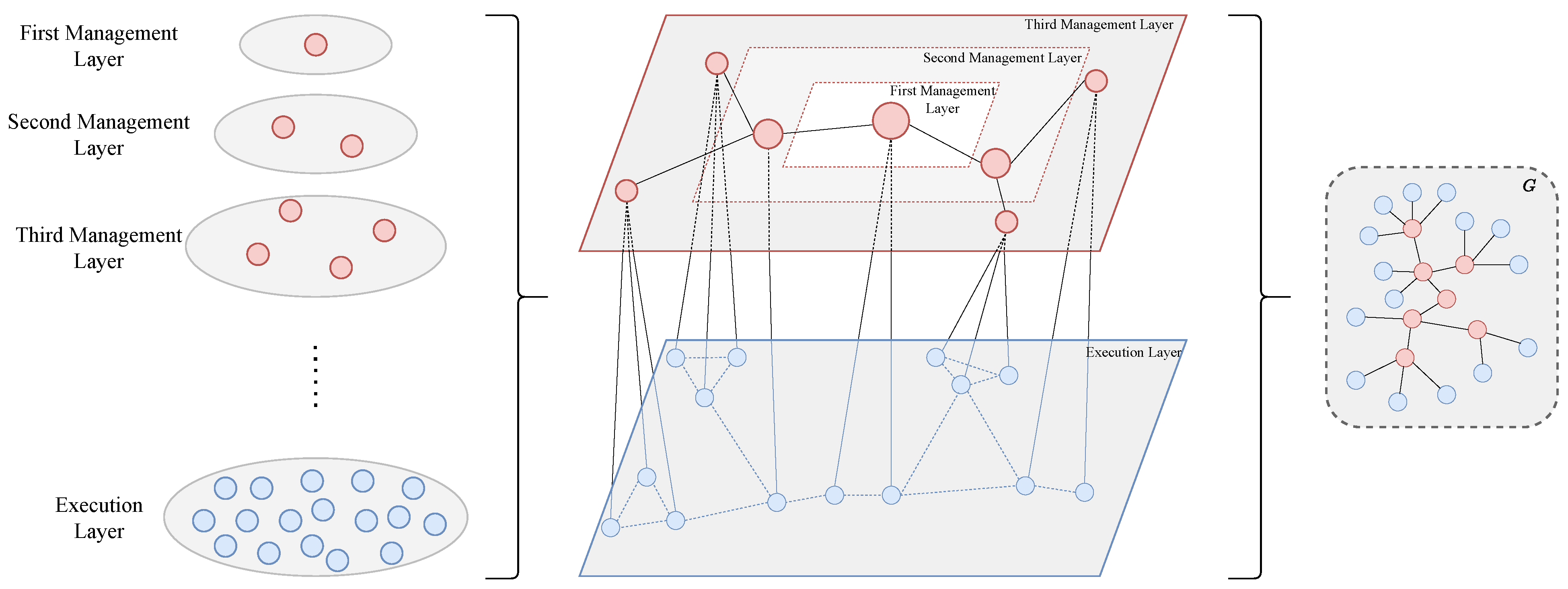
The network structure of the planning–execution network is shown in Figure 1.

The PEN has multiple management layers and an execution layer. Each node in the network is a project, including the planning project and the execution project, and there is a jurisdictional relationship between the edge representative units. Each management layer contains a series of planning projects, and the execution projects all belong to the execution layer. Projects in the management layer are arranged from top to bottom in the PEN according to their levels, and the execution layer is at the bottom.

We studied the characteristics of project group structure and found similarities with research on organizational structure. We constructed the PEN after drawing on the literature research on organizational structures [64,65,66,67] and incorporating experience in program management [68,69,70,71,72,73]. Therefore, the characteristics and construction methods of PEN are similar to those of organizational structure models. The PEN should have the following characteristics:

• The topmost management layer has only one planning project. In the management of a project group, there is generally only one top-level project. If there are multiple planning projects at the same level at the topmost level, there will be cases where the goals of the project group are not clear and specific. Therefore, all management orders should ultimately originate from the topmost planning project.
• Planning projects can manage lower-level planning projects, or manage execution projects. In the PEN, the planning project only has the functions of target planning and management, and does not undertake specific behaviors. A planning project may manage several lower-level planning projects, and may also manage several execution projects.
• The execution project can only accept the management of the planning project, and has no management function itself. An execution project is a project that is positioned to execute various specific activities and does not have the function of managing other projects, so it can only accept the management of planning projects from all levels.
• Except for the topmost planning project, each project is connected to only one superior planning project. Each planning project can be connected to multiple subordinate planning projects or execution projects. In general, a project cannot be managed by multiple projects at the same time in principle.
• There are a limited number of project layers. The management level of a project group cannot be unlimited; otherwise, the management chain will be too long, and the cycle of information transmission and feedback will be greatly lengthened. Therefore, the number of project levels in the planning–execution network needs to be limited.
• There is no mutual management relationship between planning projects at the same level. Management at the same level is likely to lead to overlapping or unclear goals among planning projects, resulting in confusion in project group management.

According to the characteristics of the above-mentioned program group, the generation rules of the planning–execution network are stipulated under the given circumstances of the planning project and the execution project.

• The topmost management layer has only one planning project, which has the highest priority.
• The number of planning projects at the lower level is higher than that at the upper level.
• A planning project must be connected to at least one adjacent planning project of a different layer.
• An upper-level planning project can be connected to multiple lower-level planning projects, and a lower-level planning project is only connected to one upper-level planning project.
• An execution project can only be connected to one planning project, and a planning project can be connected to multiple execution projects.
• Each planning project must manage at least one planning project or execution project.
• There is no management relationship between planning projects at the same level.
• The number of planning project layers is limited.

The number l of planning project levels should satisfy:

$$2\le l\le \left|P^a\right|$$

(10)

The management layer has at least 2 levels because it has been stipulated that the first level $L_1$ has only one planning project, and the rest of the planning projects are concentrated in the second level $L_2$.

The most extreme case is that each level has only one planning project, and the number of levels is equal to the number of planning items, namely $l=\left|P^a\right|$.

When generating a PEN, the number of management layers l can artificially define a range.

The representation method of PEN is an adjacency matrix. According to the definition, when the element $w_{ij}=1$ of the adjacency matrix, it means that there is a connection between two projects (there is a jurisdictional relationship); when the element $w_{ij}=0$ of the adjacency matrix, it indicates that there is no connection between the two projects (there is no jurisdictional relationship). The generated adjacency matrix W has the following form:

$$W=\left[\begin{array}{cc}C& D\\ D^T& O\end{array}\right]=\begin{array}{cc}& \begin{array}{cc}\stackrel{P^a}{\overbrace{\begin{array}{cccc}{p}_1& p_2& \cdots & p_{m_1}\end{array}}}& \stackrel{P^b}{\overbrace{\begin{array}{ccc}{p}_{m_1+1}& \cdots & p_m\end{array}}}\end{array}\\ \begin{array}{c}{P}^a\left\{\begin{array}{c}{p}_1\\ p_2\\ ⋮\\ p_{m_1}\end{array}\right.\\ P^b\left\{\begin{array}{c}{p}_{m_1+1}\\ ⋮\\ p_m\end{array}\right.\end{array}& \left[\begin{array}{cccccccc}0& 1& \cdots & 0& & 0& \cdots & 0\\ 1& 0& \cdots & 0& & 0& \cdots & 0\\ ⋮& ⋮& \ddots & ⋮& & ⋮& \ddots & ⋮\\ 0& 0& \cdots & 0& & 0& \cdots & 1\\ 0& 0& \cdots & 0& & 0& \cdots & 0\\ ⋮& ⋮& \ddots & ⋮& & ⋮& \ddots & ⋮\\ 0& 0& \cdots & 1& & 0& \cdots & 0\end{array}\right]\end{array}$$

(11)

The adjacency matrix W is a symmetric matrix which satisfies $W=W^T$. In addition, W is also a block matrix. Matrix $C_{\left|P^a\right|\times \left|P^b\right|}$ represents the adjacency relationship between planning projects, satisfying $C=C^T$; matrix $D_{\left|P^a\right|\times \left|P^b\right|}$ represents the connection relationship between planning projects and execution projects. There is no jurisdictional relationship between the execution projects, so their adjacency matrix is a zero matrix.

The program generation studied in this paper refers to various types of network structures that can be generated according to the rules of the PEN under the existing resources. Therefore, the input of the program generation stage is each project that has been determined, and the corresponding capability value of each project. The value of the project’s capability is the inherent attribute of each project, which is mainly used for program evaluation and does not affect the generation of the project group itself. The set of network programs is defined as $\mathsf{\Psi }$.

The project group network generation steps are as follows:

• Divide planning projects into different management layers, among which the highest management layer has only one planning project, and the number of planning projects in the upper layer is not higher than the number of planning projects in the lower layer.
• All planning projects are assigned a jurisdictional relationship, and all planning projects form a network. During the assignment of relationships, the network generation rules of the program need to be followed.
• Allocate the execution projects under the jurisdiction of the planning projects.

5. Network Capability Performance Indicators

5.1. Management Performance

Management capability $x_1$ is the core capability of a planning project, and the management ability of a planning project can be obtained through various methods such as project review, achievements, and expert evaluation. But this capability is only the management capability of the planning project itself, and it is the absolute planning capability of this project. When this project is put into the PEN, its management capability will be greatly reduced by the influence of the network structure. For example, when a planning project manages many other projects at the same time, especially when the number of projects managed is large, its management efficiency will be greatly reduced, because the projects it manages may have exceeded its own management capabilities; therefore, this paper proposes relative management capability indicators to measure this management capability.

First of all, from the analysis of the mechanism of project management operation, managers give instructions to the managed by sending messages and communications, and convey their own intentions to the managed projects. Therefore, the operating mechanism of management is actually a process of information interaction. The manager communicates the information to the managed, and the managed feeds back the information to the manager. Management is effective when information is delivered in a timely and effective manner. Conversely, when the information is not communicated in a timely manner and the reliability is insufficient, the ability and effect of management will be greatly reduced. When the number of projects managed by the planning project is too large, it will bear a large amount of information load. This can result in information not being communicated in a timely manner, and the reliability of information delivery will also be reduced. The result is a decline in the actual performance of the management capabilities of the PEN. Therefore, from this point of view, the ultimate cause of the insufficient level of planning and project management capability is the sharp increase in information load. We use a relative management capability to measure and evaluate this phenomenon.

In complex networks, betweenness centrality is an indicator that measures the information load of a node in a network. Betweenness centrality refers to the number of shortest paths through a network node. Using betweenness centrality, it is possible to measure the information load of a planning project. The greater the information load, the stronger the weakening of management capability; therefore, we define the relative management capability of each planning project and name this indicator as management performance.

Management performance is the relative management capability of a planning project in a PEN program. The management performance depends on the original management capability $x_1$ of the planning project itself, and also depends on the PEN structure, i.e., the amount of information carried by the planning project in this network measured by betweenness centrality.

Therefore, for the planning project $p_i\in P^a$, its betweenness centrality $B{C}_i$ in a certain network program $G_r$ is defined as [74]:

$$B{C}_i^r=\sum _{p_s\ne p_i\ne p_t}\frac{n_{st}^i}{g_{st}}$$

(12)

where $g_{st}$ denotes the total number of shortest paths from node s to node t, and $n_{st}^i$ denotes the number of paths passing through node $p_i$ among the above shortest paths.

For the planning project $p_i$, under the capability criterion $x_1$, the management capability is ${\varphi }_{i1}$ without distinguishing the decision maker. Then, management performance $M{P}_i^r$ is defined as follows:

$$M{P}_i^r=\frac{{\varphi }_{i1}}{{\left({\varphi }_{i1}\right)}^{{\overline{BC}}_i^r}}$$

(13)

Among them, ${\overline{BC}}_i^r$ is the normalized betweenness centrality, and the value range is $[0,1]$. If the betweenness centrality of the planning project is low, the value is close to 0, and the management performance of the planning project is close to the management ability; if the betweenness centrality of the planning project is high, the value of the management performance is close to 1.

5.2. Execution Performance

Execution capability is the main capability of the entire PEN, and it is also the basis for final program evaluation. Execution capability is a collection of various measurement capabilities, and the execution capability criterion set $X^B=\{x_2,\cdots ,x_k\}$.

In Section 5.1, the principle of management has been analyzed from the mechanism of information transmission, and how management performance depends on management capability and information load (measured by betweenness centrality) is discussed. Therefore, this part will continue to define the execution capability from the perspective of information transmission.

In the PEN mentioned in this paper, since the execution project is managed by the planning project, the execution capability of the execution project is affected by the planning project that manages it. That is, the management performance of the planning project linked to the execution project has an impact on the performance of the execution capability of the execution project.

In terms of information transfer, since there is only one top-level planning project in the PEN, and all instructions are essentially issued from this project, the distance between the execution project and the top-level planning project (the number of edges included in the path between two nodes in the network) also affects the capability to execute projects.

Therefore, due to the loss of timeliness and reliability caused by the transmission of instruction information from the top-level planning project downwards, as the information transmission path increases, the performance of execution capabilities will also bring about a decline. Therefore, an attenuation coefficient $\alpha \in [0,1]$ is specified to measure the attenuation of the execution capability as the information transmission path increases.

When considering attenuation, also note that not all orders originate from the topmost planning project. Some lower-level planning projects on other paths may also spontaneously generate a series of instruction information, and the link generated by this information dissemination is shorter, and the attenuation of the ability is also less.

Therefore, the executive capability of each executive project is defined, and this indicator is named executive performance. Execution performance is a demonstration of the capability to execute projects in a PEN program.

For the execution project $p_i\in P^b$ in the network program $G_r$, its execution capability performance $B{P}_{ij}^r$ on the execution capability criterion $x_j$ is defined as follows:

$$B{P}_{ij}^r={\varphi }_{ij}·M{P}_u^r·{\mathsf{\Omega }}_i$$

(14)

Among them, ${\varphi }_{ij}$ is the value of the execution project $p_i$ under a certain execution capability criterion $x_j$ without considering the decision maker. $M{P}_u^r$ is the management performance of the planning project $p_u$ that manages the execution project in the network program $G_r$. The execution project $p_u$ manages the execution project $v_i$, i.e., $w_{iu}=1$. ${\mathsf{\Omega }}_i$ is the retained amount of execution item $p_i$ after the attenuation of execution ability caused by the loss of instruction information on the path.

The decay retention ${\mathsf{\Omega }}_i$ is related to the path from the execution item $p_i$ to the topmost planning project, so it is defined as follows:

$${\mathsf{\Omega }}_i=\frac{1}{di{s}_i}\alpha +\frac{1}{di{s}_i}{\alpha }^2+\cdots +\frac{1}{di{s}_i}{\alpha }^{di{s}_i}=\frac{1}{di{s}_i}\sum _{s=1}^{di{s}_i}{\alpha }^s$$

(15)

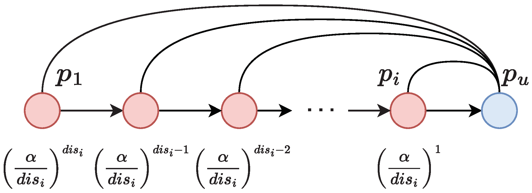
$di{s}_i$ refers to the length of the shortest path from project $p_i$ to top-level planning project $p_1$, i.e., the number of edges in the path, and this shortest path is unique. The meaning of Equation (15) refers to the attenuation of data sent by multiple nodes. Figure 2 is an information transmission path, and the information attenuation of each path is shown in Figure 2.

When the information is transmitted, every time it passes through a project, the information will decay at the decay rate of $\alpha$. Therefore, the decay degree of the planning project $p_u$ with the shortest distance from the execution project $p_u$ is $\alpha$, indicating the ratio of retained information after attenuation. When extending upward to the top-level planning project $p_1$, the path length is $di{s}_i$ after $di{s}_i$ attenuation times, so the attenuation degree is ${\alpha }^{di{s}_i}$. Assume that the probability of issuing instructions for each planning item in the upper layer is the same, so all attenuation degrees are $\{\frac{{\alpha }^1}{di{s}_i},\frac{{\alpha }^2}{di{s}_i}\cdots \frac{{\alpha }^{di{s}_i}}{di{s}_i}\}$. The summation yields Equation (15).

Under different attenuation rate values, the changing trend of the attenuation retention amount ${\mathsf{\Omega }}_i$ with the path length $di{s}_i$ is as shown in Figure 3.

Finally, the overall execution of the entire scheme $G_r$ is as follows:

$$TB{P}_j^r=\sum _{p_i\in P^b}B{P}_{ij}^r$$

(16)

6. PEN Program Evaluation Method

In Section 5, two evaluation indicators for nodes in the PEN were specified, namely management performance and execution performance. The final program evaluation will be calculated based on these two indicators. Specific PEN solution evaluation is divided into three steps: input processing, capability performance calculation, and solution evaluation ranking.

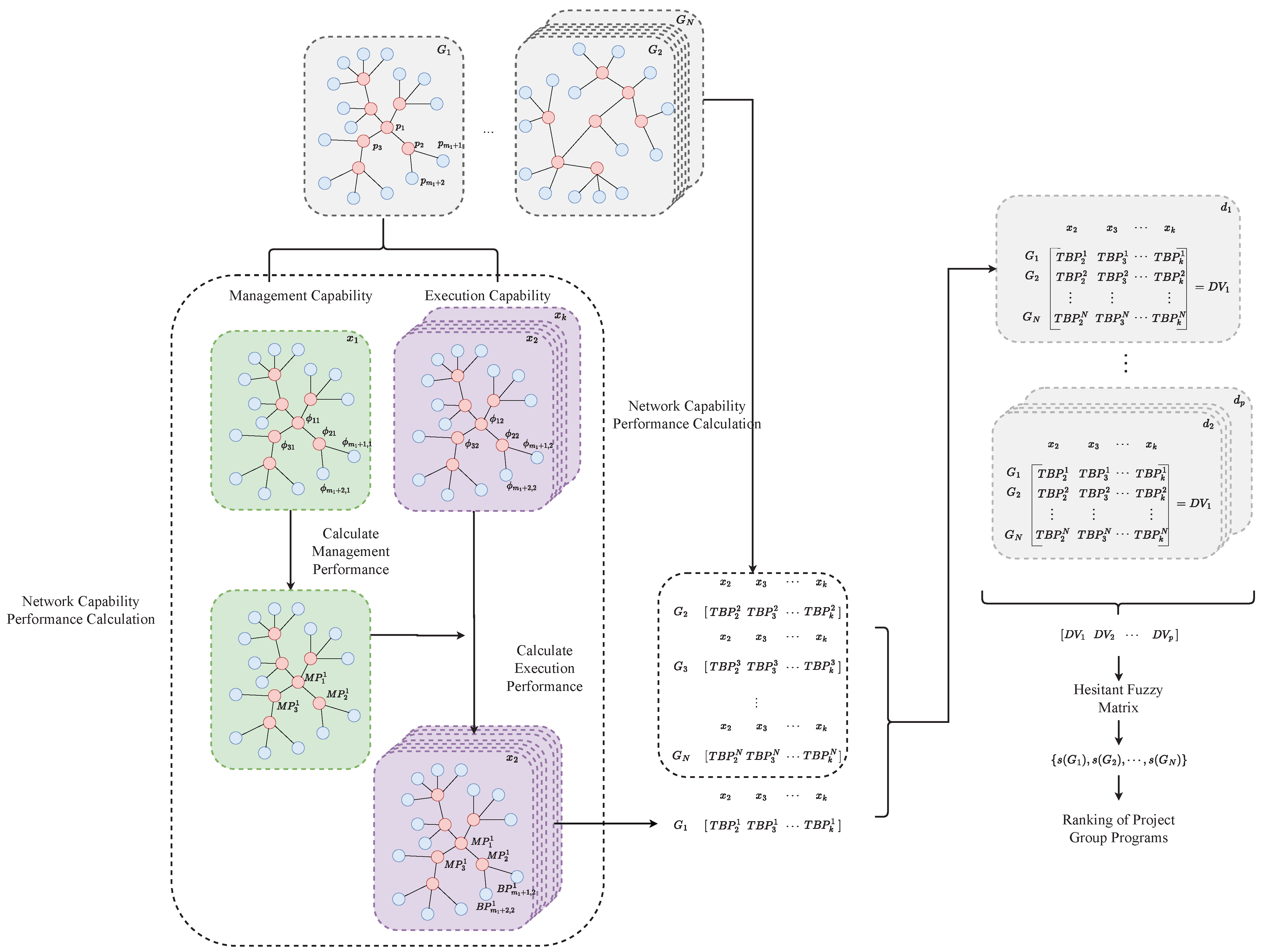
This chapter will describe the program evaluation method in detail. The main process is shown in Figure 4.

Figure 4 shows the entire process of project group program evaluation. First, the network is sliced according to capability types to obtain the management capability network and a series of execution capability networks. Then the management capability is calculated, and on this basis the execution capability is calculated. After obtaining the total execution capabilities of a series of project group network programs, an evaluation matrix is formed to rank the programs.

6.1. Input Processing

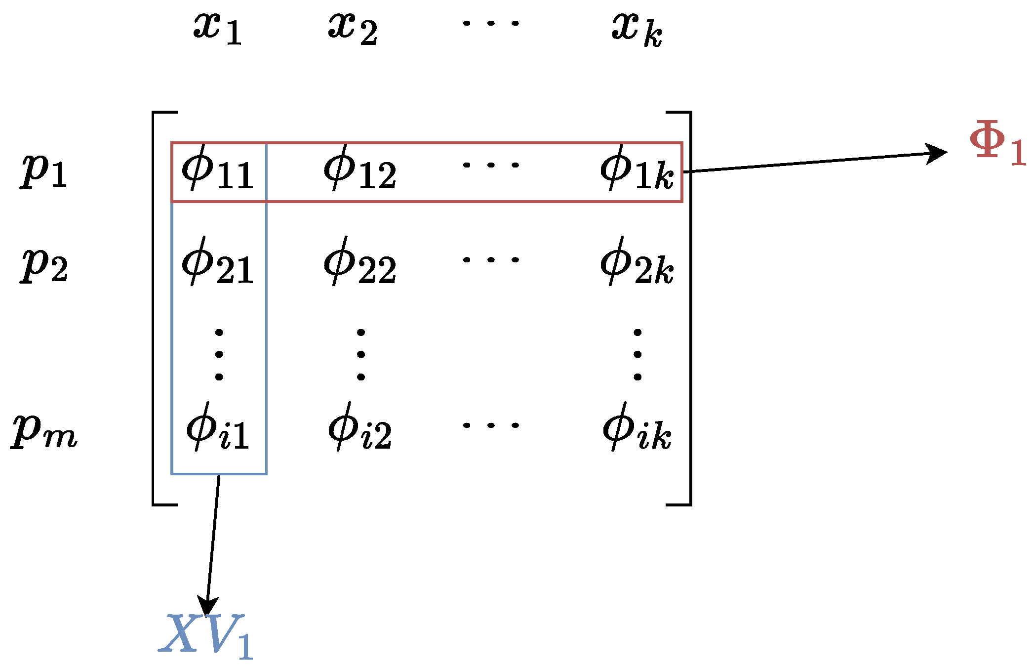
For a project $p_i$, its capability value set under the criterion X is ${\Phi }_i=\{{\varphi }_{i1},{\varphi }_{i2},cdots,{\varphi }_{ik}\}$. This is a collection of values based on the capabilities of each project. In order to facilitate subsequent index calculations, the capability values are now combined into a set with reference to each capability criterion. Then, under the ability $x_j$, the ability value set of each project is $X{V}_j=\{{\varphi }_{1j},{\varphi }_{2j},\cdots ,{\varphi }_{mj}\}$.

In particular, $X{V}_1$ represents the value set of management capabilities of all projects. $X{V}_2,\cdots X{V}_k$ is the set of values of all projects in execution capability.

The decomposition process of the input data is shown in Figure 5.

6.2. Management Performance Calculation

In the process of input decomposition in Section 6.1, the management capability value set $X{V}_1$ of all projects is obtained. Taking $X{V}_1=\{{\varphi }_{11},{\varphi }_{21},\cdots ,{\varphi }_{m1}\}$ as input according to Equations (12) and (13), we can calculate the management performance of all planning projects under the project group network program $G_r$. Since the value of the management capability of the execution project in $X{V}_1$ is 0, there is no need to calculate the management performance of the execution project. All planning projects $P^a=\{p_1,p_2,\cdots ,p_{m_1}\}$ management performance value set is $\{M{P}_1^r,M{P}_2^r,\cdots ,M{P}_{m_1}^r\}$.

6.3. Execution Performance Calculation

According to the obtained management performance and the capability value sets $X{V}_2,\cdots ,X{V}_k$ of all projects under each criterion set, each execution project under the project group network program can be calculated separately from the set of execution performance, $\{B{P}_{m_1+1,2}^r$, $B{P}_{m_1+2,2}^r$, ⋯, $B{P}_{m,2}^r\}$, $\{B{P}_{m_1+1,3}^r$, $B{P}_{m_1+2,3}^r$, ⋯, $B{P}_{m,3}^r\}$, $\{B{P}_{m_1+1,k}^r$, $B{P}_{m_1+2,k}^r$, ⋯, $B{P}_{m,k}^r\}$.

Finally, according to the above execution performance set, under the project group network program, the followng execution performance set of the entire network can be obtained: $\{TB{P}_2^r,TB{P}_3^r,\cdots ,TB{P}_k^r\}$.

The execution performance of each network program constructed in the previous section constitutes an evaluation matrix $DV$:

$$DV={\left({\overline{TBP}}_j^r\right)}_{N\times k}=\left[\begin{array}{cccc}\overline{TB{P}_2^1}& \overline{TB{P}_3^1}& \cdots & \overline{TB{P}_k^1}\\ \overline{TB{P}_2^2}& \overline{TB{P}_3^2}& \cdots & \overline{TB{P}_k^2}\\ ⋮& ⋮& & ⋮\\ \overline{TB{P}_2^N}& \overline{TB{P}_3^N}& \cdots & \overline{TB{P}_k^N}\end{array}\right]$$

(17)

where ${\overline{TBP}}_j^r$ is the value normalized by each column of the matrix, representing the normalized value of the network program $G_r$ execution performance under the execution capability criterion $x_j$.

Since decision makers have different evaluation values for the capabilities of each project, each decision maker under the decision maker set $D=\{d_1,d_2,\cdots ,d_p\}$ will generate an evaluation matrix eventually, and the final evaluation matrix set is $\{D{V}_1$, $D{V}_2$, ⋯, $D{V}_p\}$.

The elements in the evaluation matrix are the degrees of affiliation when the hesitant fuzzy method is finally used for program evaluation. Finally, using the hesitant fuzzy method, the score set $\{s\left(G_1\right),s\left(G_2\right),\cdots ,s\left(G_{N^{\prime }}\right)\}$ of each network program can be obtained and completely evaluated.

7. Case Study

7.1. Case Description

In order to study the effectiveness of program generation and hesitant fuzzy program evaluation method based on project group network, a case study of project group is proposed.

In the case of our research project group, there are 17 different projects, of which 6 are planning projects and the rest are execution projects. The project group plans to set up three management layers. Referring to the practice in the field of project management, we use seven capability criteria $X=\{x_1,x_2,x_3,x_4,x_5,x_6,x_7\}$ for each project measured. The seven main capabilities are as follows: management capability $x_1$, advancing progress capability $x_2$, communication and coordination capability $x_3$, risk prevention and control capability $x_4$, quality supervision capability $x_5$, market research capability $x_6$, and staff training capability $x_7$. See

Table 2. Introduction to project capabilities.

Capability Name	Meaning
Management Capability	It refers to the capability of planning projects to reasonably convey various information and notices to subordinate projects, rationally dispatch resources, and guide the normal progress of subordinate projects.
Advancing Progress Capability	According to the project content of the planning project, the capability to gradually complete the relevant tasks within the specified time period and steadily promote the progress of the project.
Communication and Coordination Capability	The capability to communicate and cooperate with other project participants and project external collaborators to solve problems.
Risk Prevention and Control Capability	The capability to execute projects against possible hazards brought about by various emergencies, ensure the normal operation of project funds, and the steady development of various tasks.
Quality Supervision Capability	The capability to complete the task content of the project in accordance with the quality standards of the planning project.
Market Research Capability	The execution project is based on the current market and field status, understands the field dynamics, adjusts the technical details accordingly, and updates the ability of the development method.
Staff Training Capability	Train new members for the project team and enrich the capabilities of project team members.

for specific explanations and meanings.

By inviting experts in relevant fields and practitioners who have been involved in project management for a long time, the performance of each project under each capability criterion is evaluated. The evaluation results of three decision-making experts $D=\{d_1,d_2,d_3\}$ with high reference value are selected as the basis for subsequent program evaluation. Under the evaluation of the three experts, the values of the capability indicators of each unit are shown in

Table 3. Table of capability values for each project.

		Capability Criteria
Project Type and Number		${\mathit{x}}_{\mathbf{1}}$	${\mathit{x}}_{\mathbf{2}}$	${\mathit{x}}_{\mathbf{3}}$	${\mathit{x}}_{\mathbf{4}}$	${\mathit{x}}_{\mathbf{5}}$	${\mathit{x}}_{\mathbf{6}}$	${\mathit{x}}_{\mathbf{7}}$
Planning Project	$p_1$	10, 12, 9	0, 0, 0	0, 0, 0	0, 0, 0	0, 0, 0	0, 0, 0	0, 0, 0
	$p_2$	6, 6, 8	0, 0, 0	0, 0, 0	0, 0, 0	0, 0, 0	0, 0, 0	0, 0, 0
	$p_3$	6, 6, 8	0, 0, 0	0, 0, 0	0, 0, 0	0, 0, 0	0, 0, 0	0, 0, 0
	$p_4$	4, 3, 3	0, 0, 0	0, 0, 0	0, 0, 0	0, 0, 0	0, 0, 0	0, 0, 0
	$p_5$	4, 3, 3	0, 0, 0	0, 0, 0	0, 0, 0	0, 0, 0	0, 0, 0	0, 0, 0
	$p_6$	4, 3, 3	0, 0, 0	0, 0, 0	0, 0, 0	0, 0, 0	0, 0, 0	0, 0, 0
Execution Project	$p_7$∼$p_{14}$	0, 0, 0	10, 12, 8	10, 9, 12	10, 7, 8	5, 3, 7	2, 3, 4	1, 2, 3
	$p_{15}$	0, 0, 0	5, 8, 3	15, 12, 18	5, 4, 3	20, 25, 30	0, 3, 0	0, 1, 0
	$p_{16}$	0, 0, 0	5, 5, 5	5, 3, 6	10, 12, 8	10, 7, 3	20, 25, 30	5, 3, 8
	$p_{17}$	0, 0, 0	0, 1, 1	10, 8, 10	5, 5, 3	0, 1, 2	0, 1, 2	20, 15, 25

.

Table 3 shows an evaluation by experts of the performance of each project under each capability. The evaluation value of each expert does not set a range of values, which are all subjective judgments based on experience, so there is no comparison between the absolute values of evaluations by different experts. Subsequently, by normalizing the scores of each expert, relative values with research significance can be obtained for comparison.

There are two types of execution projects: basic execution projects ($p_7$∼$p_{14}$) and special execution projects ($p_{15},p_{16},p_{17}$). The number of basic execution projects is relatively large, and they are the main body of the execution projects. The special execution projects are mainly used to complete some guarantee tasks with little demand.

The basic execution project is the most common execution project in the project group. Basic execution projects are used to complete the most important and large requirements in the project group. In the case of this paper, the most prominent capability item of the basic execution project is capability $x_2$ “Advancing Progress Capability”. This is also the most important and basic capability of a project group. The capabilities of the basic execution projects are not particularly outstanding in other aspects, so they need to be supplemented by other execution projects.

Special execution projects are mainly used to meet some special capabilities that are necessary but not in high demand. These projects are more outstanding in a certain capability. For example, project $p_{15}$ has a higher value on capability $x_5$ “Quality Supervision Capability”.

7.2. Program Evaluation

7.2.1. Generate Network Program

We generate all possible program according to the project group network generation method. There are three management layers. The first management layer assigns a planning project with the highest management capability, which is determined as $p_1$. The latter two management layers randomly assign planning projects, and according to the second rule, ensure that the number of planning projects in the third layer is greater than that in the second layer.

According to rules 5 and 8, basic execution projects cannot subsequently be assigned to the highest management level, nor can special professional execution projects be assigned to the lowest management level. You cannot have a planning project without a subordinate planning project or execution project. During the allocation process, execution projects of the same type and with exactly the same attributes can be regarded as the same repeated projects; without distinction in allocation, they can be regarded as the same “puzzle” in the ”mosaic”.

According to the above rules, after the allocation of 6 planning projects, there are 10 allocation programs in total. Subsequently, the management relationship between planning projects is generated, and finally 60 kinds of planning project structure programs are generated. Then the basic execution projects are allocated, and the eight execution projects are allocated to the planning projects on the second and third levels for management. There is no difference between the 8 execution projects when allocating, so there are 495 allocation programs in total. Finally, the three special execution projects are allocated to the planning projects on the first and second management layers, and there are 27 allocation programs in total. Therefore, a total of 60 × 495 × 27 = 801,900 network programs are finally generated, and the program numbers are $G_1$∼$G_{801900}$.

7.2.2. Manage Performance and Execution Performance Calculation

According to the calculation methods in Section 5.1 and Section 5.2, the evaluation matrix composed of three experts is obtained as follows:

$$D{V}_1=\begin{array}{cc}& \begin{array}{cccccc}{\overline{TBP}}_2& {\overline{TBP}}_3& {\overline{TBP}}_4& {\overline{TBP}}_5& {\overline{TBP}}_6& {\overline{TBP}}_7\end{array}\\ \begin{array}{c}{G}_1\\ G_2\\ G_3\\ \cdots \\ G_{801899}\\ G_{801900}\end{array}& \left[\begin{array}{cccccc}0.497& 0.578& 0.547& 0.587& 0.540& 0.566\\ 0.502& 0.607& 0.565& 0.607& 0.562& 0.666\\ 0.517& 0.599& 0.568& 0.660& 0.620& 0.521\\ \cdots & \cdots & \cdots & \cdots & \cdots & \cdots \\ 0.538& 0.612& 0.585& 0.748& 0.718& 0.424\\ 0.557& 0.663& 0.622& 0.685& 0.637& 0.677\end{array}\right]\end{array}$$

$$D{V}_2=\begin{array}{cc}& \begin{array}{cccccc}{\overline{TBP}}_2& {\overline{TBP}}_3& {\overline{TBP}}_4& {\overline{TBP}}_5& {\overline{TBP}}_6& {\overline{TBP}}_7\end{array}\\ \begin{array}{c}{G}_1\\ G_2\\ G_3\\ \cdots \\ G_{801899}\\ G_{801900}\end{array}& \left[\begin{array}{cccccc}0.506& 0.565& 0.573& 0.583& 0.565& 0.577\\ 0.514& 0.592& 0.598& 0.611& 0.591& 0.659\\ 0.526& 0.583& 0.602& 0.668& 0.643& 0.541\\ \cdots & \cdots & \cdots & \cdots & \cdots & \cdots \\ 0.546& 0.592& 0.629& 0.770& 0.736& 0.462\\ 0.569& 0.647& 0.657& 0.689& 0.666& 0.680\end{array}\right]\end{array}$$

$$D{V}_3=\begin{array}{cc}& \begin{array}{cccccc}{\overline{TBP}}_2& {\overline{TBP}}_3& {\overline{TBP}}_4& {\overline{TBP}}_5& {\overline{TBP}}_6& {\overline{TBP}}_7\end{array}\\ \begin{array}{c}{G}_1\\ G_2\\ G_3\\ \cdots \\ G_{801899}\\ G_{801900}\end{array}& \left[\begin{array}{cccccc}0.504& 0.572& 0.536& 0.554& 0.548& 0.581\\ 0.512& 0.599& 0.551& 0.575& 0.574& 0.664\\ 0.522& 0.595& 0.556& 0.611& 0.616& 0.548\\ \cdots & \cdots & \cdots & \cdots & \cdots & \cdots \\ 0.538& 0.613& 0.574& 0.677& 0.695& 0.473\\ 0.565& 0.655& 0.607& 0.643& 0.644& 0.686\end{array}\right]\end{array}$$

7.2.3. Synthesizing the Hesitant Fuzzy Matrix and Ranking the Programs

It is determined that the importance of the three experts is the same, and the above evaluation matrix is synthesized into a hesitant fuzzy matrix, as shown in

Table 4. Hesitation fuzzy matrix.

	${\overline{\mathit{TBP}}}_2$	${\overline{\mathit{TBP}}}_3$	${\overline{\mathit{TBP}}}_4$	${\overline{\mathit{TBP}}}_5$	${\overline{\mathit{TBP}}}_6$	${\overline{\mathit{TBP}}}_7$
$G_1$	0.497, 0.506, 0.504	0.578, 0.565, 0.572	0.547, 0.573, 0.536	0.587, 0.583, 0.554	0.540, 0.565, 0.548	0.566, 0.577, 0.581
$G_2$	0.502, 0.514, 0.512	0.607, 0.592, 0.599	0.565, 0.598, 0.551	0.607, 0.611, 0.575	0.562, 0.591, 0.574	0.666, 0.659, 0.664
$G_3$	0.517, 0.526, 0.522	0.599, 0.583, 0.595	0.568, 0.602, 0.556	0.660, 0.668, 0.611	0.620, 0.643, 0.616	0.521, 0.541, 0.548
…	…	…	…	…	…	…
$G_{801899}$	0.538, 0.546, 0.538	0.612, 0.592, 0.613	0.585, 0.629, 0.574	0.748, 0.770, 0.677	0.718, 0.736, 0.695	0.424, 0.462, 0.473
$G_1$	0.557, 0.569, 0.565	0.663, 0.647, 0.655	0.622, 0.657, 0.607	0.685, 0.687, 0.643	0.637, 0.666, 0.644	0.677, 0.680, 0.686

.

Each row represents a network program, each column represents the overall performance of the entire network program under a certain criterion, and ${\overline{TBP}}_2$ represents the entire project group of each program under the criterion $x_2$, which is the normalized value of execution performance. The three values in the cell correspond to the normalized execution performance calculated from the initial assessments of three experts.

In this case, it is considered that the weight of each criterion is the same, so the weight vector is $w={(\frac{1}{6},\frac{1}{6},\frac{1}{6},\frac{1}{6},\frac{1}{6},\frac{1}{6})}^T$. According to Formula (5), the HFWA operator is used to calculate the hesitant fuzzy element $h_i(i=1,2,3,\cdots$, 801,900) of the program $G_i(i=1,2,3,\cdots$, 801,900):

$$\begin{array}{c}{h}_1=HFWA(h_{11},h_{12},h_{13},h_{14},h_{15},h_{16})\\ =HFA(h_{11},h_{12},h_{13},h_{14},h_{15},h_{16})\\ =\{0.497,0.506,0.504\},\{0.578,0.565,0.572\},\\ \{0.547,0.573,0.536\},\{0.578,0.583,0.554\},\\ \{0.540,0.565,0.548\},\{0.566,0.577,0.581\}\\ =\frac{1}{6}\oplus h_{1i}={\displaystyle \bigcup _{{\gamma }_{11}\in h_{11},{\gamma }_{12}\in h_{12},{\gamma }_{13}\in h_{13},{\gamma }_{14}\in h_{14},{\gamma }_{15}\in h_{15},{\gamma }_{16}\in h_{16}}}\left\{1-{\displaystyle \prod _{i=1}^6}{(1-{\gamma }_{1i})}^{\frac{1}{4}}\right\}\\ =\{\underset{l_h=729}{\underbrace{0.553,0.555,0.556,\cdots ,0.550}}\}\end{array}$$

The same can be said of

$$h_2=\{\underset{l_h=729}{\underbrace{0.588,0.587,0.588,\cdots ,0.582}}\}$$

$$h_3=\{\underset{l_h=729}{\underbrace{0.584,0.587,0.588,\cdots ,0.576}}\}$$

$$\cdots$$

$$h_{801899}=\{\underset{l_h=729}{\underbrace{0.619,0.623,0.625,\cdots ,0.603}}\}$$

$$h_{801900}=\{\underset{l_h=729}{\underbrace{0.643,0.643,0.644,\cdots ,0.635}}\}$$

Subsequently, the score s and deviation degree $\overline{\sigma }$ of each program solution are calculated according to Formula (6), and we obtain:

$$s\left(h_1\right)=0.5552,s\left(h_2\right)=0.5890,s\left(h_3\right)=0.5859,\cdots ,s\left(h_{801899}\right)=0.6204,s\left(h_{801900}\right)=0.6438$$

$\begin{array}{c}\overline{\sigma }\left(h_1\right)=1.88\times {10}^{-5},\overline{\sigma }\left(h_2\right)=2.30\times {10}^{-5},\overline{\sigma }\left(h_3\right)=4.34\times {10}^{-5},\cdots ,\hfill \\ \overline{\sigma }\left(h_{801899}\right)=1.20\times {10}^{-4},\overline{\sigma }\left(h_{801900}\right)=3.25\times {10}^{-5},\hfill \end{array}$

According to the scores of the above programs, the final set of programs with the highest score ($s=1$) is as follows:

$$\begin{array}{c}\{G_{570780},G_{572292},G_{584718},G_{585270},G_{585657},G_{591303},G_{594954},G_{597591},G_{604425},G_{608211},G_{610875},G_{625056},\hfill \\ G_{625473},G_{625833},G_{637686},G_{639198},G_{664935},G_{665514},G_{671574},G_{675225},G_{677835},G_{684642},G_{688455},G_{705327},\hfill \\ G_{705744},G_{706077},G_{717930},G_{719442},G_{745449},G_{745947},G_{751845},G_{755550},G_{765156},G_{768888},G_{785598},G_{786069}\}\hfill \end{array}$$

There are a total of 37 programs in the above program collection. These 37 programs are all the best ones selected by the hesitant fuzzy method. These optimal programs represent the optimal project group network structure under the evaluation method proposed in this article. We will explain this structure in detail with examples in Section 7.3.

7.3. Analysis of Network Programs Evaluation Results

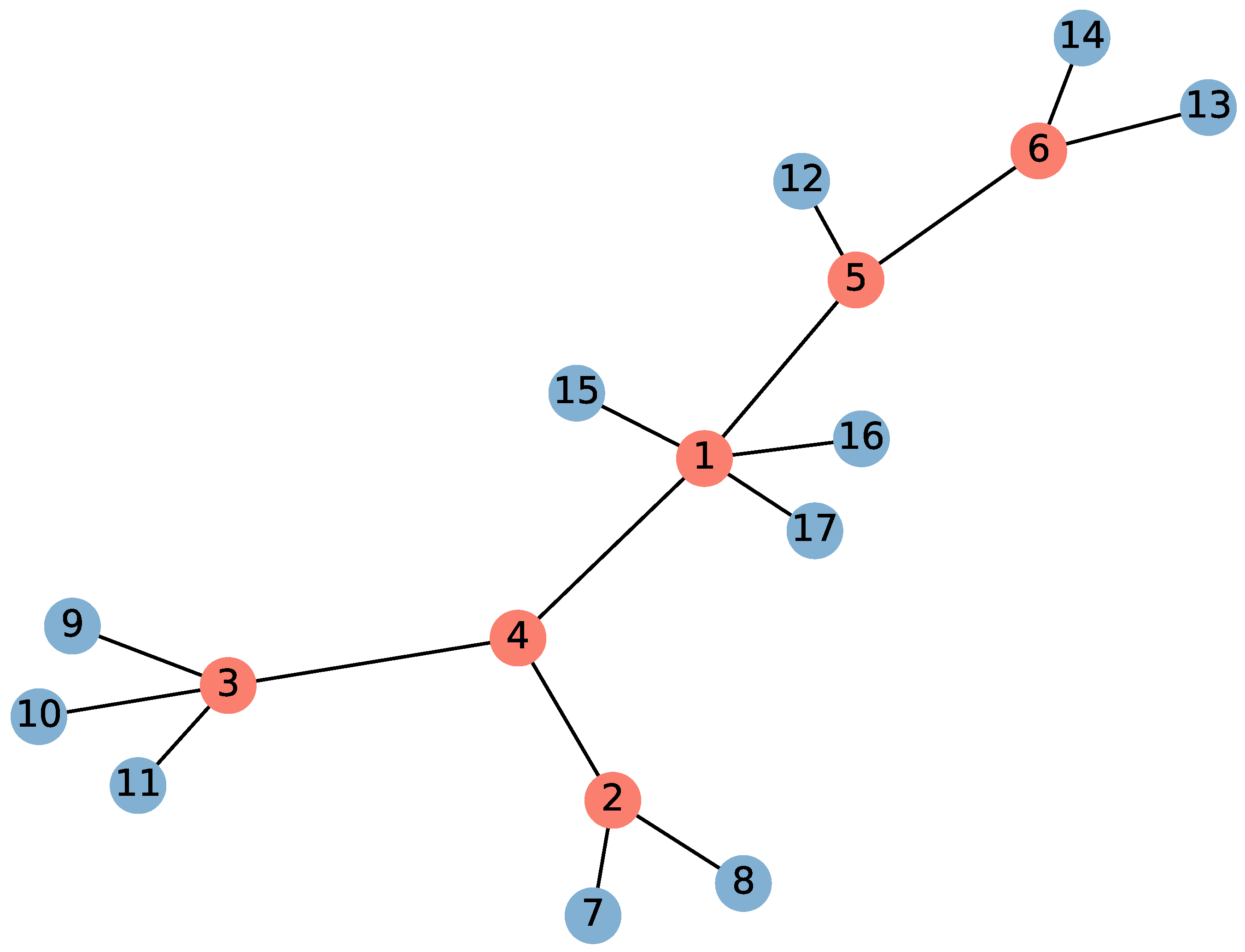
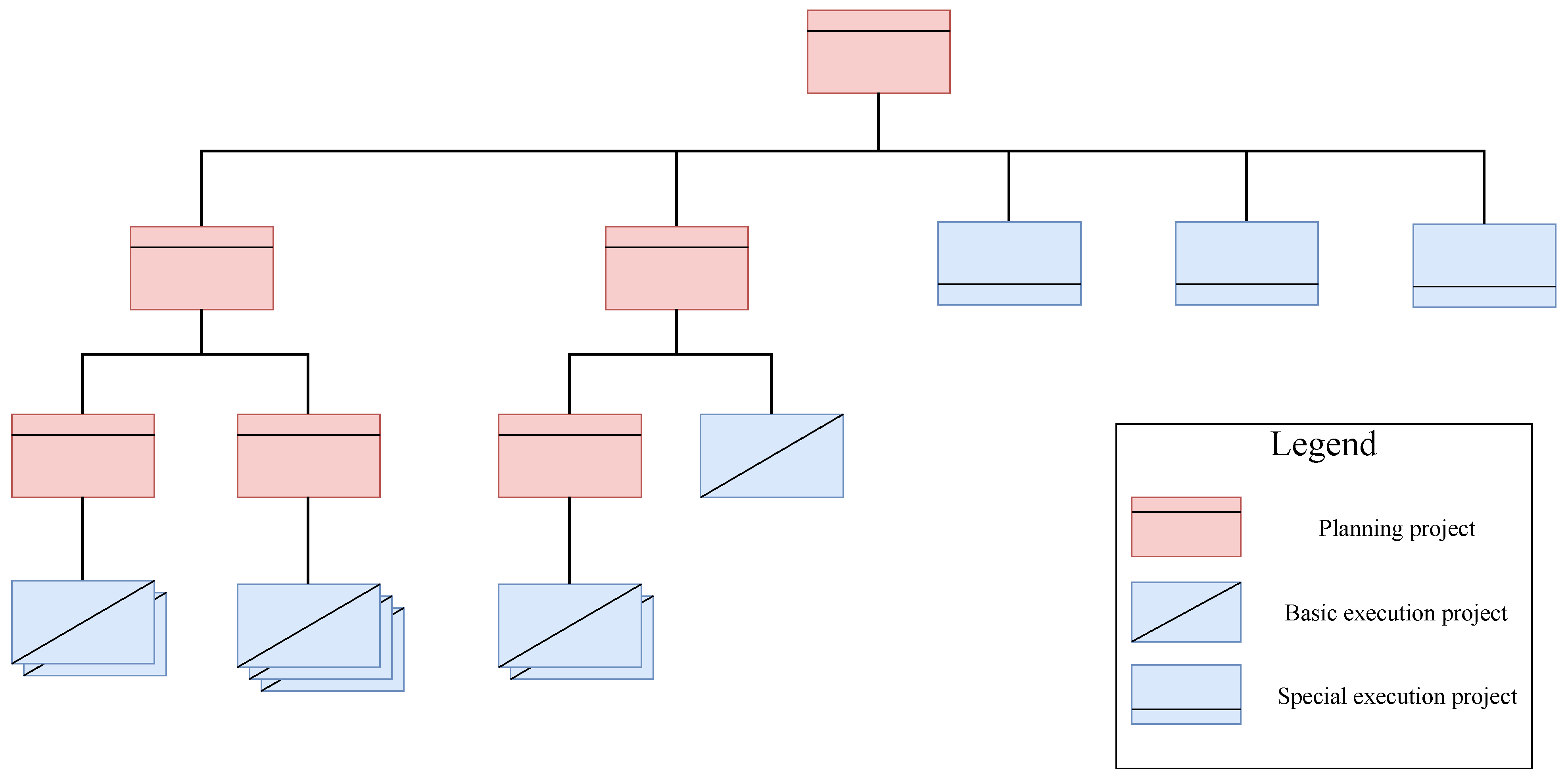
Take scheme $G_{570780}$ as an example; the program finally generates an adjacency matrix, which is a symmetric matrix. The network graph drawn according to the adjacency matrix is shown in Figure 6 and Figure 7.

The project network diagram above shows the final organization of project group program. The numbers in the nodes are project numbers. Red nodes represent planning projects, and blue nodes represent execution projects.

The project group organization diagram is a structured representation of the project group’s final solution. The red unit is the planning project. Its position in the organizational diagram represents the layer of the planning project. From top to bottom, it is the first, second, and third management layer, respectively. The blue units are execution projects, which are basic execution projects and special execution projects, both of which belong to the execution layer. The connection relationships in the organization diagram represent the jurisdictional relationships among the project groups.

• Average management load. In the method of this paper, except for the five projects managed by the top planning project $p_1$, the number of projects directly managed by other planning projects is generally two to three. This avoids the unbalanced information load situation in which some planning projects have too much management information load and some planning projects have less load, which helps to fully involve to the execution capability of each project in the overall project group.
• Basic execution project management decentralization. The basic execution projects are mainly managed by the third-level planning projects. The planning projects $p_2$, $p_3$ and $p_6$ of the third management layer manage seven of the eight execution projects, and only one execution project is added to the second-level planning projects. The number of basic execution projects is relatively large, and they are also the backbone of the entire project group. The basic execution projects are delegated to the management of low-level planning projects. Although the link of information transmission is increased and part of the execution performance of the execution projects is sacrificed, it helps to reduce the information load and management pressure of upper-level planning projects, thus enabling the entire project group program to have better overall execution performance.
• Special execution projects are directly under the topmost planning project. Special execution projects are not the main force in project execution, but they have some special execution skills during project execution. These special capabilities are often necessary for the operation of project groups and are an important part of ensuring the normal operation of project groups. And because the number of these special execution projects is relatively small, in order to ensure the full play of these capabilities, these special execution projects are often handed over to higher-level planning project management as a direct subordinate team. The above-mentioned optimal program embodies this principle. When the high-level planning project management capability is sufficient, a small number of special execution projects can be properly managed to improve the overall execution capability.

After analyzing and comparing 36 optimal plans, excluding duplication of plans caused by units of the same type but with different numbers, it was concluded that there are two categories of optimal organization programs:

• General organization program: The program represented by the above-described program $G_{570780}$. It is characterized by the fact that three special execution projects are directly under the jurisdiction and management of the highest-level planning project. The remaining basic execution projects are mainly managed by the lowest-level planning project, with a few directly managed by higher-level planning projects, and the information load is evenly managed.
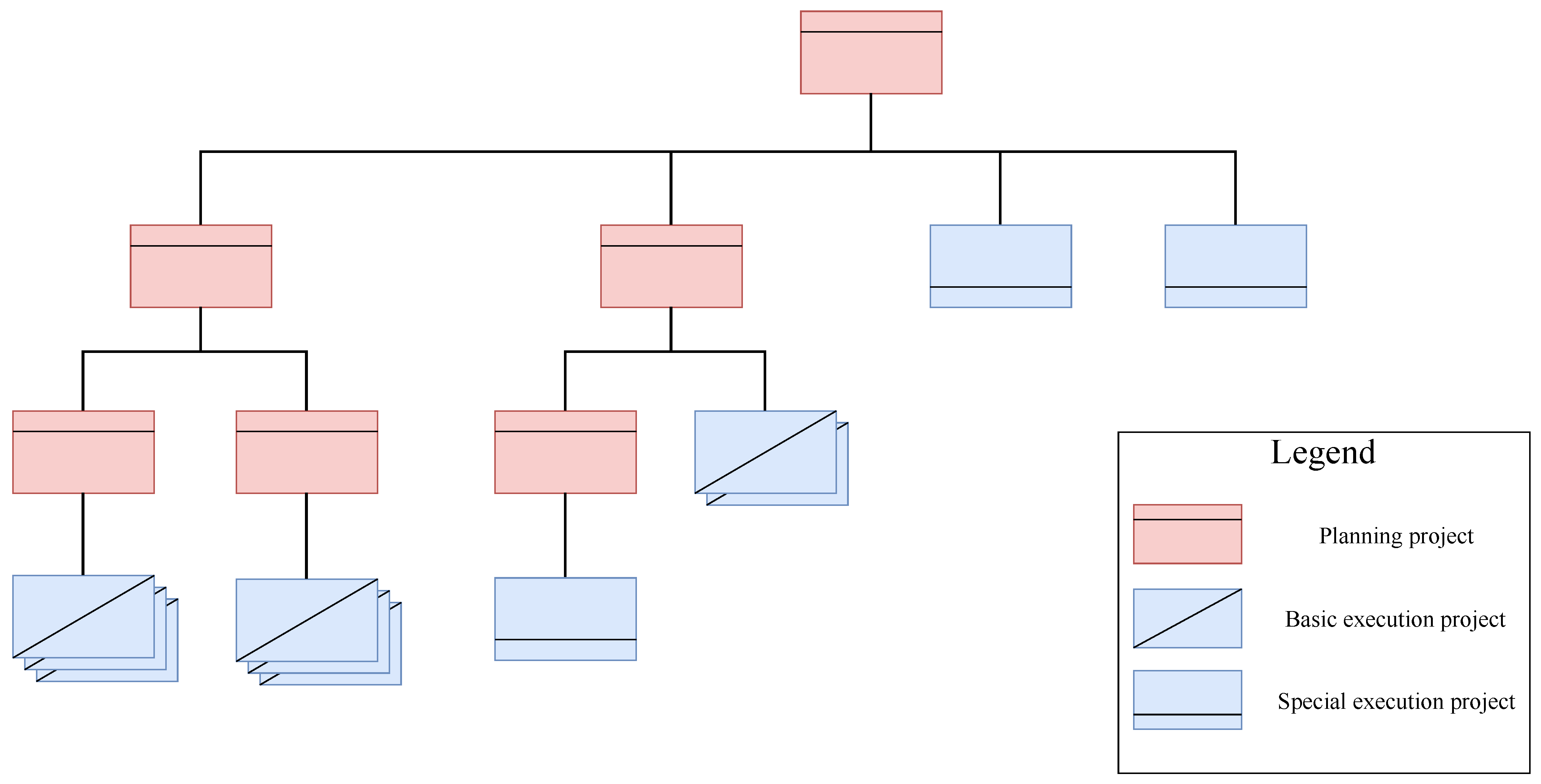
• Specialized organization program: The plan represented by plan $G_{785598}$. The characteristic is that the top-level planning project only has special execution projects under its jurisdiction, and it has two planning projects under its jurisdiction. One of the second-level planning projects has two third-level planning projects under its jurisdiction, and each has three general execution projects under its jurisdiction; the other second-level planning project has two general execution projects and one third-level planning project under its jurisdiction directly under the jurisdiction of a certain special execution project to strengthen the performance of the special execution capability of the special execution project. The program network diagram of this program is shown in Figure 8.

The above example puts a special execution project under the independent command of a third-level planning project to individually strengthen its execution performance, so that the plan can better exert the professional capabilities of the sub-special operations unit. Special execution programs here are also replaceable.

Although the two types of optimal programs—the general program and the specialized program—have the same score in the end, the characteristics and emphases of the two programs are not the same. This also provides ideas for the construction of project group programs.

In addition to the 36 optimal programs analyzed, there are a total of 24 programs with the lowest score ($s=0.3265$), which are as follows:

$$\begin{array}{c}\{G_{13351},G_{26716},G_{31184},G_{53446},G_{57914},G_{71279},G_{93541},G_{106906},G_{133636},G_{173731},G_{187096},G_{213826},\hfill \\ G_{253921},G_{267286},G_{294016},G_{325214},G_{338579},G_{365309},G_{405404},G_{418769},G_{445499},G_{485594},G_{498959},G_{525689}\}\hfill \end{array}$$

Taking scheme $G_{13351}$ as an example, we analyze the characteristics of the program with the lowest score. The network structure diagram of the program $G_{13351}$ is shown in Figure 9.

In this program, almost all execution projects and planning projects are concentrated under the management of planning project $p_2$, which results in other planning projects being unable to play their due management roles, and the management burden of $p_2$ is too heavy. Therefore, the entire program cannot properly execute its role. This is the drawback of excessive centralization.

8. Conclusions

Combining coupling network and hesitant fuzzy decision-making theory, this paper proposes a project group evaluation and decision-making method. Firstly, the concept of PEN is proposed, and the project group is modeled and described through the coupling network, and the nature, constraint rules and generation method of the project group network program are obtained; secondly, based on the characteristics of the PEN, combined with the network evaluation indicators, the attribute of each network node is aggregated into the evaluation attribute of the entire program network, and the evaluation value of each network program under multiple capability attributes can be obtained. Finally, according to the evaluation basis of different experts for each program, the capability values calculated above are used to obtain the hesitant fuzzy matrix, and the scores of each program are obtained through corresponding calculations and sorted by preference, thereby assisting in decision-making.

This method designs a set of modeling evaluation systems and standards for the project group, which can effectively evaluate the project program. However, the modeling evaluation method in this paper still has some shortcomings:

• The program space is huge. As the number of nodes increases, the program summary will grow exponentially. This case has only 17 network nodes, and there are 801,900 solutions according to the constraint rules. Therefore, it is necessary to study the solution generation method more deeply to avoid duplication of solutions and to use optimization algorithms for solution optimization.
• There are many optimal solutions. Since there is no significant difference in the evaluation of the execution capabilities of each project by various experts, the final evaluation results of multiple programs are the same. However, the optimal plan of project group itself is diverse, and more optimal projects can also provide more options.

Based on the existing problems of this research, in the next step of work, the following research will be focused on the following:

• Exploring methods for screening and pruning during proposal generation to reduce the size of the proposal space.
• Further adding constraints and rules in line with the actual situation to reduce the number of optimal solutions and avoid repeated solutions as much as possible.

Our work studied the application of the hesitant fuzzy method in project group evaluation and decision-making, and verified the effectiveness through cases, and also put forward certain suggestions for project group design.

Our work applies the hesitant fuzzy multi attribute decision making method in the evaluation of project group programs. A project group is modeled using a multi-layer coupling network to classify projects into planning projects and execution projects. The overall performance of the program is calculated using the topology of the network and the characteristics of the project group management information, using the hesitant fuzzy method to evaluate program options and obtain the final preference ranking of options.

Project group management is also an important topic in public governance. Scientific methods of project group management can help build smart cities and digital governments, prevent major public emergencies caused by project failures, and help improve public governance capabilities.

References

- Sharif, R.A.; Pokharel, S. Smart City Dimensions and Associated Risks: Review of literature. Sustain. Cities Soc. 2022, 77, 103542. [Google Scholar] [CrossRef]
- Liu, Y.; Wei, J.; Rodriguez, A.F.C. Development of a strategic value assessment model for smart city. Int. J. Mob. Commun. 2014, 12, 346–359. [Google Scholar] [CrossRef]
- Heerkens, G.R. Project Management; McGraw Hill Professional: New York, NY, USA, 2002. [Google Scholar]
- Carruthers, J.A.; Battersby, A. Advances in Critical Path Methods. J. Oper. Res. Soc. 1966, 17, 359–380. [Google Scholar] [CrossRef]
- Nasution, S.H. Fuzzy Critical Path Method. IEEE Trans. Syst. Man Cybern. 1994, 24, 48–57. [Google Scholar] [CrossRef]
- Baits, H.A.; Puspita, I.A.; Bay, A.F. Combination of program evaluation and review technique (PERT) and critical path method (CPM) for project schedule development. Int. J. Integr. Eng. 2020, 12, 68–75. [Google Scholar] [CrossRef]
- Cottrell, W.D. Simplified program evaluation and review technique (PERT). J. Constr. Eng. Manag. 1999, 125, 16–22. [Google Scholar] [CrossRef]
- Zhang, X.; Liu, W. Complex Equipment Remanufacturing Schedule Management Based on Multi-Layer Graphic Evaluation and Review Technique Network and Critical Chain Method. IEEE Access 2020, 8, 108972–108987. [Google Scholar] [CrossRef]
- Zhou, L.; Xie, J.; Gu, X.; Lin, Y.; Ieromonachou, P.; Zhang, X. Forecasting return of used products for remanufacturing using Graphical Evaluation and Review Technique (GERT). Int. J. Prod. Econ. 2016, 181, 315–324. [Google Scholar] [CrossRef]
- Devi, T.R.; Reddy, V.S. Work breakdown structure of the project. Int. J. Eng. Res. Appl. 2012, 2, 683–686. [Google Scholar]
- Tausworthe, R.C. The work breakdown structure in software project management. J. Syst. Softw. 1979, 1, 181–186. [Google Scholar] [CrossRef]
- Haugan, G.T. Effective Work Breakdown Structures; Berrett-Koehler Publishers: Oakland, CA, USA, 2001. [Google Scholar]
- Fleming, Q.W.; Koppelman, J.M. Earned value management. Cost Eng. 2002, 44, 32–36. [Google Scholar]
- Mahmoudi, A.; Bagherpour, M.; Javed, S.A. Grey Earned Value Management: Theory and Applications. IEEE Trans. Eng. Manag. 2021, 68, 1703–1721. [Google Scholar] [CrossRef]
- Christensen, D.S. The Costs and Benefits of the Earned Value Management Process. J. Parametr. 1998, 18, 1–16. [Google Scholar] [CrossRef]
- Reusch, P.J. Extending project management processes. In Proceedings of the 2015 IEEE 8th International Conference on Intelligent Data Acquisition and Advanced Computing Systems: Technology and Applications (IDAACS), Warsaw, Poland, 24–26 September 2015; Volume 2, pp. 511–514. [Google Scholar] [CrossRef]
- Loehr, K.; Khan, R.A. Project finance—On new standards for processes in project and program management. In Proceedings of the 6th IEEE International Conference on Intelligent Data Acquisition and Advanced Computing Systems, Prague, Czech Republic, 15–17 September 2011; Volume 2, pp. 901–905. [Google Scholar] [CrossRef]
- Ojeda, O.; Reusch, P. Sustainable procurement—Extending project procurement concepts and processes based on PMBOK. In Proceedings of the 2013 IEEE 7th International Conference on Intelligent Data Acquisition and Advanced Computing Systems (IDAACS), Berlin, Germany, 12–14 September 2013; Volume 2, pp. 530–536. [Google Scholar] [CrossRef]
- Boonstra, A.; Reezigt, C. A Complexity Framework for Project Management Strategies. Proj. Manag. J. 2023, 54, 253–267. [Google Scholar] [CrossRef]
- Wu, Y.; Li, J.; Wang, J.; Huang, Y. Project portfolio management applied to building energy projects management system. Renew. Sustain. Energy Rev. 2012, 16, 718–724. [Google Scholar] [CrossRef]
- Lou, T.; He, B.; Zhang, B.; Duan, Z. Research and Application of BIM Project Group Management. IOP Conf. Ser. Earth Environ. Sci. 2019, 218, 012056. [Google Scholar] [CrossRef]
- Cheng, J.; Wang, H. Application and Popularization of BIM Technology in Project Management. Appl. Mech. Mater. 2012, 174, 2871–2875. [Google Scholar] [CrossRef]
- Rust, C. Getting Kicks From Route 66. Continental 2001, 5, 53–55. [Google Scholar]
- Mulva, S.P. ARIES: A Theoretical Framework for Evaluating Aspects of Enterprise Sustainability; Georgia Institute of Technology: Atlanta, GA, USA, 2004. [Google Scholar]
- Keller, R.T. Predictors of the Performance of Project Groups in R & Organizations. Acad. Manag. J. 1986, 29, 715–726. [Google Scholar] [CrossRef]
- Chevrier, S. Cross-cultural management in multinational project groups. J. World Bus. 2003, 38, 141–149. [Google Scholar] [CrossRef]
- Gevers, J.M.; van Eerde, W.; Rutte, C.G. Time pressure, potency, and progress in project groups. Eur. J. Work Organ. Psychol. 2001, 10, 205–221. [Google Scholar] [CrossRef]
- Murata, T. Comparison of Inter-Layer Couplings of Multilayer Networks. In Proceedings of the 2015 11th International Conference on Signal-Image Technology & Internet-Based Systems (SITIS), Bangkok, Thailand, 23–27 November 2015; pp. 448–452. [Google Scholar] [CrossRef]
- Kumar, T.; Narayanan, M.; Ravindran, B. Effect of Inter-layer Coupling on Multilayer Network Centrality Measures. J. Indian Inst. Sci. 2019, 99, 237–246. [Google Scholar] [CrossRef] [PubMed]
- Wang, L.; Jia, X.; Pan, X.; Xia, C. Extension of synchronizability analysis based on vital factors: Extending validity to multilayer fully coupled networks. Chaos Solitons Fractals 2021, 142, 110484. [Google Scholar] [CrossRef]
- Jiang, C.; Zhang, Y.; Wang, H.; Zhou, Y.; Zou, Y. Study on coupled social network public opinion communication based on improved SEIR. In Proceedings of the 2020 IEEE Intl Conf on Parallel & Distributed Processing with Applications, Big Data & Cloud Computing, Sustainable Computing & Communications, Social Computing & Networking (ISPA/BDCloud/SocialCom/SustainCom), Exeter, UK, 17–19 December 2020; pp. 1495–1500. [Google Scholar] [CrossRef]
- Wang, G.; Liu, Y.; Li, J.; Tang, X.; Wang, H. Superedge coupling algorithm and its application in coupling mechanism analysis of online public opinion supernetwork. Expert Syst. Appl. 2015, 42, 2808–2823. [Google Scholar] [CrossRef]
- Zhang, Y.; Feng, Y. Two-Layer Coupled Network Model for Topic Derivation in Public Opinion Propagation. China Commun. 2020, 17, 176–187. [Google Scholar] [CrossRef]
- Daley, D.J.; Kendall, D.G. Epidemics and Rumours. Nature 1964, 204, 1118. [Google Scholar] [CrossRef]
- Han, Q.; Shi, K.; Gu, M.; You, L.; Miao, F. Modeling Repeated Rumor Spreading in Coupled Social Networks. IEEE Access 2021, 9, 89732–89740. [Google Scholar] [CrossRef]
- Ju, C.; Wang, C.; Jiang, Y.; Bao, F.; Zhou, H.; Xu, C. Exploring a Multi-Layer Coupled Network Propagation Model Based on Information Diffusion and Bounded Trust. Int. J. Public Health 2022, 67, 1604887. [Google Scholar] [CrossRef]
- Wang, W.; Tang, M.; Zhang, H.F.; Lai, Y.C. Dynamics of social contagions with memory of nonredundant information. Phys. Rev. E 2015, 92, 012820. [Google Scholar] [CrossRef]
- Jiang, S.; Fan, H. Credit risk contagion coupling with sentiment contagion. Phys. A Stat. Mech. Its Appl. 2018, 512, 186–202. [Google Scholar] [CrossRef]
- Huang, J.; Luo, K.; Cao, L.; Wen, Y.; Zhong, S. Learning Multiaspect Traffic Couplings by Multirelational Graph Attention Networks for Traffic Prediction. IEEE Trans. Intell. Transp. Syst. 2022, 23, 20681–20695. [Google Scholar] [CrossRef]
- Ye, B.; Shi, X.; Li, D.; Gao, C. The Impact of Multi-energy Complementary System on the Reliability of Energy Supply of Distribution. In Proceedings of the 2018 International Conference on Power System Technology (POWERCON), Guangzhou, China, 6–8 November 2018; pp. 1459–1464. [Google Scholar] [CrossRef]
- Tian, X.; Zhouhong, L.; Zhaoguang, P.; Hongbin, S. Modeling and Simulation for Multi Energy Flow Coupled Network Computing. In Proceedings of the 2018 International Conference on Power System Technology (POWERCON), Guangzhou, China, 6–8 November 2018; pp. 992–998. [Google Scholar] [CrossRef]
- Shu, P.; Wang, W.; Tang, M.; Do, Y. Numerical identification of epidemic thresholds for susceptible-infectedrecovered model on finite-size networks. Chaos 2015, 25, 063104. [Google Scholar] [CrossRef] [PubMed]
- Boguñá, M.; Castellano, C.; Pastor-Satorras, R. Nature of the epidemic threshold for the susceptible-infected-susceptible dynamics in networks. Phys. Rev. Lett. 2013, 111, 068701. [Google Scholar] [CrossRef] [PubMed]
- Castellano, C.; Pastor-Satorras, R. Thresholds for epidemic spreading in networks. Phys. Rev. Lett. 2010, 105, 2187014. [Google Scholar] [CrossRef] [PubMed]
- Barthélemy, M.; Barrat, A.; Pastor-Satorras, R.; Vespignani, A. Velocity and hierarchical spread of epidemic outbreaks in scale-free networks. Phys. Rev. Lett. 2004, 92, 18–21. [Google Scholar] [CrossRef]
- Cui, A.X.; Wang, W.; Tang, M.; Fu, Y.; Liang, X. Efficient allocation of heterogeneous response times in information spreading process. Chaos 2014, 24, 033113. [Google Scholar] [CrossRef]
- Lei, Y.; Jiang, X.; Guo, Q.; Ma, Y.; Li, M.; Zheng, Z. Contagion processes on the static and activity-driven coupling networks. Phys. Rev. E 2016, 93, 032308. [Google Scholar] [CrossRef]
- Haak, D.M.; Fath, B.D.; Forbes, V.E.; Martin, D.R.; Pope, K.L. Coupling ecological and social network models to assess “transmission” and “contagion” of an aquatic invasive species. J. Environ. Manag. 2017, 190, 243–251. [Google Scholar] [CrossRef]
- Zadeh, L. Information and control. Fuzzy Sets 1965, 8, 338–353. [Google Scholar]
- Torra, V. Hesitant fuzzy sets. Int. J. Intell. Syst. 2010, 25, 529–539. [Google Scholar] [CrossRef]
- Xia, M.; Xu, Z. Hesitant fuzzy information aggregation in decision making. Int. J. Approx. Reason. 2011, 52, 395–407. [Google Scholar] [CrossRef]
- Shen, Q.; Lou, J.; Liu, Y.; Jiang, Y. Hesitant fuzzy multi-attribute decision making based on binary connection number of set pair analysis. Soft Comput. 2021, 25, 14797–14807. [Google Scholar] [CrossRef] [PubMed]
- Gong, Z.; Wang, J. Hesitant fuzzy graphs, hesitant fuzzy hypergraphs and fuzzy graph decisions. J. Intell. Fuzzy Syst. 2021, 40, 865–875. [Google Scholar] [CrossRef]
- Meng, L.; Li, L. Time-sequential hesitant fuzzy set and its application to multi-attribute decision making. Complex Intell. Syst. 2022, 8, 4319–4338. [Google Scholar] [CrossRef]
- Yu, D.; Li, D.F.; Merigó, J.M. Dual hesitant fuzzy group decision making method and its application to supplier selection. Int. J. Mach. Learn. Cybern. 2016, 7, 819–831. [Google Scholar] [CrossRef]
- Lin, R.; Zhao, X.; Wang, H.; Wei, G. Hesitant fuzzy linguistic aggregation operators and their application to multiple attribute decision making. J. Intell. Fuzzy Syst. 2014, 27, 49–63. [Google Scholar] [CrossRef]
- Zhang, J.L.; Qi, X.W. Research on multiple attribute decision making under hesitant fuzzy linguistic environment with application to production strategy decision making. Adv. Mater. Res. 2013, 753–755, 2829–2836. [Google Scholar] [CrossRef]
- Qian, G.; Wang, H.; Feng, X. Generalized hesitant fuzzy sets and their application in decision support system. Knowl.-Based Syst. 2013, 37, 357–365. [Google Scholar] [CrossRef]
- Liu, H.; Rodríguez, R.M. A fuzzy envelope for hesitant fuzzy linguistic term set and its application to multicriteria decision making. Inf. Sci. 2014, 258, 220–238. [Google Scholar] [CrossRef]
- Liao, H.; Xu, Z.; Zeng, X.J. Novel correlation coefficients between hesitant fuzzy sets and their application in decision making. Knowl.-Based Syst. 2015, 82, 115–127. [Google Scholar] [CrossRef]
- Xu, Z.; Xia, M. Induced generalized intuitionistic fuzzy operators. Knowl.-Based Syst. 2011, 24, 197–209. [Google Scholar] [CrossRef]
- Chen, N.; Xu, Z.; Xia, M. Correlation coefficients of hesitant fuzzy sets and their applications to clustering analysis. Appl. Math. Model. 2013, 37, 2197–2211. [Google Scholar] [CrossRef]
- Torra, V.; Narukawa, Y. On hesitant fuzzy sets and decision. In Proceedings of the 2009 IEEE International Conference on Fuzzy Systems, Jeju, Republic of Korea, 20–24 August 2009; pp. 1378–1382. [Google Scholar] [CrossRef]
- Lynne Markus, M. Information technology and organizational structure. In Computing Handbook—Information Systems and Information Technology; Chapman and Hall: London, UK, 2014; Volume 16, pp. 444–459. [Google Scholar] [CrossRef]
- Structures, O. The Structuring of Organizational Structures Stewart Ranson, Bob Hinings and Royston Greenwood. Science 1980, 25, 1–18. [Google Scholar]
- Carter, E. Party organization and leadership. Extrem. Right West. Eur. 2012, 230, 64–100. [Google Scholar] [CrossRef]
- Scott, W.R. Organizational Structure. Annu. Rev. Sociol. 1956, 1, 1–20. [Google Scholar] [CrossRef]
- Kuster, J.; Bachmann, C.; Hubmann, M.; Lippmann, R.; Schneider, P. Project Management Handbook; Springer: Berlin/Heidelberg, Germany, 2023. [Google Scholar]
- Khatib, M.E.; Alhosani, A.; Alhosani, I.; Matrooshi, O.A.; Salami, M. Simulation in Project and Program Management: Utilization, Challenges and Opportunities. Am. J. Ind. Bus. Manag. 2022, 12, 731–749. [Google Scholar] [CrossRef]
- Ika, L.A.; Pinto, J.K. The “re-meaning” of project success: Updating and recalibrating for a modern project management. Int. J. Proj. Manag. 2022, 40, 835–848. [Google Scholar] [CrossRef]
- Guo, K.; Zhang, L. Multi-objective optimization for improved project management: Current status and future directions. Autom. Constr. 2022, 139, 104256. [Google Scholar] [CrossRef]
- Arefazar, Y.; Nazari, A.; Hafezi, M.R.; Maghool, S.A.H. Prioritizing agile project management strategies as a change management tool in construction projects. Int. J. Constr. Manag. 2022, 22, 678–689. [Google Scholar] [CrossRef]
- Kerzner, H. Project Management Case Studies; John Wiley & Sons: Hoboken, NJ, USA, 2022. [Google Scholar]
- Freeman, L.C. A Set of Measures of Centrality Based on Betweenness. Sociometry 1977, 40, 35. [Google Scholar] [CrossRef]