Homogeneity Test for Multiple Semicontinuous Data with the Density Ratio Model

Abstract

The density ratio model has been widely used in many research fields. To test the homogeneity of the model, the empirical likelihood ratio test (ELRT) has been shown to be valid. In this paper, we conduct a parametric test procedure. We transform the hypothesis of homogeneity to one on the equality of mean parameters of the exponential family of distributions. Then, we propose a modified Wald test and give its asymptotic power. We further apply it to the semicontinuous case when there is an excess of zeros in the sample. The simulation studies show that the new test controls the type-I error better than ELRT while retaining competitive power. Benefiting from the simple closed form of the test statistic, the computational cost is small. We also use a real data example to illustrate the effectiveness of our test.

1. Introduction

The density ratio model (DRM) was first introduced by Anderson [1] and later popularized by Qin and Zhang [2], who found the relationship between the two-sample DRM and the logistic regression model in case–control studies. The DRM models in a semi-parametric way the difference between two independent samples. Assume that $X_{01},X_{02},\cdots ,X_{0n_0}$ and $X_{11},X_{12},\cdots ,X_{1n_1}$ are two samples independently drawn from two cumulative distribution functions $G_0$ and $G_1$. The DRM postulates that

$$d{G}_1\left(x\right)=exp(\alpha +{\beta }^{\top }\mathbf{q}\left(x\right))d{G}_0\left(x\right),$$

(1)

where $\mathbf{q}\left(x\right)$ is a d-dimensional pre-specified basis function while $\alpha$ and $\beta$ are unknown parameters. We can also generalize the DRM to the $(m+1)$ sample case as follows

$$\begin{array}{cc}\hfill & X_{01},X_{02},\cdots ,X_{0n_0}\sim G_0\left(x\right),\hfill \\ \hfill & X_{11},X_{12},\cdots ,X_{1n_1}\sim G_1\left(x\right),\hfill \\ \hfill & ⋮\hfill \\ \hfill & X_{m1},X_{m2},\cdots ,X_{m{n}_m}\sim G_m\left(x\right),\hfill \end{array}$$

(2)

where

$$d{G}_i\left(x\right)=exp({\alpha }_i+{\beta }_i^{\top }\mathbf{q}\left(x\right))d{G}_0\left(x\right),$$

for $i=1,2,\cdots ,m$. Even though the form of $g_i\left(x\right)=d{G}_i\left(x\right)$ is unspecified, many parametric distribution families are in the DRM, including normal, exponential, and gamma distributions, among others.

Due to its flexibility and utility, increasing importance has been attached to the DRM. Zhang [3] proposed a weighted Kolmogorov–Smirnov type statistic to test the validity of the DRM based on case–control data. Qin [4] and Zou et al. [5] applied the DRM to the semi-parametric mixture model and developed test statistics based on the empirical likelihood function. Zhang [6] induced the quantile estimator under a two-sample semi-parametric model and Chen and Liu [7] generalized the estimator to the $(m+1)$-sample case. Another problem of interest is to test the homogeneity of the DRM model, that is, to test whether $G_0=G_1=\cdots =G_m$. Fokianos et al. [8] outlined a method based on the classical normal-based one-way analysis of variance. Cai et al. [9] studied the properties of the dual empirical likelihood ratio tests to general hypotheses on parameters. Moreover, let $G_0$ be the initial cumulative distribution function (cdf) of a population, and $G_1$ be the cdf of the weighted distribution of $G_0$, so that their densities are connected to each other as follows,

$$g_1\left(x\right)=\frac{w\left(x\right)}{E\left[w\right(x\left)\right]}{g}_0\left(x\right).$$

Then, $w\left(x\right)$, in the context of the DRM, seems to be $e^{\alpha +{\beta }^{\top }\mathbf{q}\left(x\right)}$, and X is a random variable with density $g_0\left(x\right)$. Thus, the DRM lies in the context of weighted distributions which have many applications in various fields. The problem of detecting or estimating the weight function $w\left(x\right)$ is of interest in the framework of weighted distributions; see Patil and Rao [10], Rao [11,12] and Lele and Keim [13].

Recent research on the DRM mainly considered using the empirical likelihood function. We give a brief introduction to this method below. Given ${\alpha }_0=0$ and ${\beta }_0=\mathbf{0}$, the likelihood function of the model (2) has the form

$$\begin{array}{cc}\hfill L& =\prod _{i=0}^m\prod _{j=1}^{n_i}d{G}_i\left(x_{ij}\right)\hfill \\ \hfill & =\prod _{i=0}^m\prod _{j=1}^{n_i}exp({\alpha }_i+{\beta }_i^{\top }\mathbf{q}\left(x_{ij}\right))d{G}_0\left(x_{ij}\right).\hfill \end{array}$$

If $G_0$ is restricted to a discretized distribution as

$$G_0\left(x\right)=\sum _{i=0}^m\sum _{j=1}^{n_i}{p}_{ij}I(x_{ij}\le x),$$

where $p_{ij}$ is constrained by

$$p_{ij}>0and\sum _{i=0}^m\sum _{j=1}^{n_i}{p}_{ij}exp({\alpha }_t+{\beta }_t^{\top }\mathbf{q}\left(x_{ij}\right))=1,$$

for $t=0,1,\cdots ,m$. Then, the Lagrangian multipliers described in Qin and Lawless [14] are used to obtain the maximum empirical likelihood estimate of $({\alpha }_i,{\beta }_i)$. However, the type-I error of the empirical likelihood ratio test cannot be well controlled in finite samples. To deal with this problem, Wang et al. [15] suggested using a nonparametric bootstrap procedure. However, the computational cost of the bootstrap procedure is non-negligible, especially when m is large.

We also notice that there is increasing interest in the case when there are zero values in the samples. This phenomenon happens in many research fields such as meteorology, health, economics, and life sciences; see Tu and Zhou [16], Muralidharan and Kale [17] and Kassahun-Yimer et al. [18]. For example, in the meteorology study, a group of zero observations may correspond to a number of dry days when there are no rainfall measurements recorded. Another example happens in dietary intake studies, where zero observations may occur for some food components that are consumed episodically. In the examples mentioned above, samples are constructed from two parts. One is the zero observations and the other is the positive observations. This kind of distribution is also called a semicontinuous distribution, which has the form

$$F\left(x\right)=pI(x=0)+(1-p)I(x>0)G\left(x\right),X\ge 0,$$

where p indicates the probability of drawing a zero observation and $G\left(x\right)$ is a positive and continuous distribution. We recommend the reviews of Neelon et al. [19,20] for more details. In this paper, we adopt the DRM, as the choice of $G\left(x\right)$ benefits from the advantages we introduced above. Thus, the model becomes

$$\begin{array}{cc}\hfill & X_{01},X_{02},\cdots ,X_{0n_0}\sim F_0\left(x\right),\hfill \\ \hfill & X_{11},X_{12},\cdots ,X_{1n_1}\sim F_1\left(x\right),\hfill \\ \hfill & ⋮\hfill \\ \hfill & X_{m1},X_{m2},\cdots ,X_{m{n}_m}\sim F_m\left(x\right),\hfill \end{array}$$

(3)

where

$$F_i\left(x\right)=p_{i}I(x=0)+(1-p_i)I(x>0)G_i\left(x\right),x\ge 0$$

for $i=0,1,2,\cdots ,m$, where I is the indicator function.

A two-part test is proposed to test the homogeneity of the model (3), which is a fundamental problem in real applications. For example, the different distributions of precipitation in certain areas among years may influence the strategy of agricultural irrigation. Furthermore, in colorectal cancer clinical trials, it is important to compare the efficacy and safety between two or more treatment arms; see Lachenbruch [21], Su et al. [22], Smith et al. [23] and Wang and Tu [24]. The two-part test consists of a test for the binomial distribution and another for the continuous responses. For the two-sample case, Wang et al. [15] suggested that the former test is a ${\chi }^2$ test while the latter can be a Wilcoxon–Mann–Whitney rank-sum test or a two-sample t-test. For the $(m+1)$-sample case, the latter can be replaced by a Kruskal–Wallis rank-sum test or an ANOVA F-test; see for example, Wilcox [25], Hallstrom [26] and Pauly et al. [27]. However, as far as we are concerned, the tests mentioned above may perform badly in heteroskedastic cases.

In this paper, we propose an efficient method based on the exponential family of distributions. First, the problem of testing the homogeneity is transformed to testing the equalities of the mean parameters. Secondly, a Wald test statistic is proposed to test the equalities. Since $g_0$ is unknown, we modify the Wald test statistic based on the sample from $g_0$. This modified statistic has a simple closed form and we show that it converges in distribution to the ${\chi }^2$ distribution under the null hypotheses. We also give the local asympotical power. Thirdly, the Bernoulli distribution can be regarded as a DRM and we obtain the combined modified Wald test for the semicontinuous case. Finally, the simulation studies illustrate that the computational cost of the modified Wald test is much less than the bootstrap procedure, while it always controls type-I error better than the empirical likelihood ratio test. Moreover, the power of the modified Wald test is competitive.

The rest of the paper is organized as follows. In Section 2, we propose the method for testing the homogeneity of the two-sample model for both continuous and semicontinuous distributions. In Section 3, we generalize the result to multiple-sample cases. We illustrate the performance of the modified Wald test and compare it with the empirical likelihood ratio test through simulations in Section 4. We consider a real data sample to show the practicability of our method and give the conclusions in the last section.

2. Two-Sample Case

2.1. Density Ratio Model

In this section, we assume that $X_{01},X_{02},\cdots ,X_{0n_0}$ and $X_{11},X_{12},\cdots ,X_{1n_1}$ are the two independent samples drawn from $G_0\left(x\right)$ and $G_1\left(x\right)$, respectively. It is further assumed that for certain d-dimensional $\mathbf{q}\left(x\right)={(q_1\left(x\right),q_2\left(x\right),\cdots ,q_d\left(x\right))}^{\top }$,

$$g_1\left(x\right)=e^{\alpha +{\beta }^{\top }\mathbf{q}\left(x\right)}{g}_0\left(x\right),$$

where $g_1\left(x\right)$ and $g_0\left(x\right)$ are the density of $G_1\left(x\right)$ and $G_0\left(x\right)$ with respect to a $\sigma$-finite measure $\nu$, respectively. The hypotheses for testing the homogeneity are

$$H_0:g_0=g_1\mathrm{vs}.H_1:g_0\ne g_1.$$

(4)

Since $g_1\left(x\right)$ is a density function, we have

$$\int e^{\alpha +{\beta }^{\top }\mathbf{q}\left(x\right)}{g}_0\left(x\right)d\nu \left(x\right)=e^{\alpha }\int e^{{\beta }^{\top }\mathbf{q}\left(x\right)}{g}_0\left(x\right)d\nu \left(x\right)=1.$$

Hence, there is a function $A\left(\beta \right)$ such that

$$e^{\alpha }=e^{-A\left(\beta \right)}.$$

Then,

$$g\left(x\right)=e^{{\beta }^{\top }\mathbf{q}\left(x\right)-A\left(\beta \right)}{g}_0\left(x\right).$$

Construct an exponential family of distributions

$$\mathcal{P}=\{e^{{\beta }^{\top }\mathbf{q}\left(x\right)-A\left(\beta \right)}{g}_0\left(x\right),\beta \in {\mathsf{\Omega }}_0\},$$

(5)

where

$${\mathsf{\Omega }}_0=\left\{\beta :\int e^{{\beta }^{\top }\mathbf{q}\left(x\right)}{g}_0\left(x\right)d\nu \left(x\right)<\infty \right\}$$

is the natural parameter space. Under the family $\mathcal{P}$, the hypotheses (4) are equivalent to

$$H_0:\beta =\mathbf{0}\mathrm{vs}.H_1:\beta \ne \mathbf{0}.$$

(6)

For family $\mathcal{P}$, we give two simple assumptions.

Assumption 1.

$\mathcal{P}$ is a full-rank exponential family of distributions.

Then, under Assumption 1, the Fisher information matrix of $\mathcal{P}$ is positively definite and continuous. By the properties of the exponential family,

$$I\left(\beta \right)=co{v}_{\beta }\left(\mathbf{q}\left(x\right)\right)>0,$$

for an interior point $\beta$ of ${\mathsf{\Omega }}_0$.

Assumption 2.

The origin $\mathbf{0}$ is an interior point of ${\mathsf{\Omega }}_0$.

Although always $\mathbf{0}\in {\mathsf{\Omega }}_0$ because $g_0\left(x\right)$ is a density, it may not be an interior point. For example, if $d=1$, $q\left(x\right)=x^4$ and $g_0\left(x\right)=\varphi \left(x\right)$, the density of the standard normal distribution, then ${\mathsf{\Omega }}_0=(-\infty ,0]$.

Hypotheses (6) are expressed by the nature parameter $\beta$ of $\mathcal{P}$. We further want to represent them with the mean parameter of $\mathcal{P}$, which is defined as

$$m\left(\beta \right)=E_{\beta }\left(\mathbf{q}\left(x\right)\right)={\int }_{-\infty }^{\infty }\mathbf{q}\left(x\right)e^{{\beta }^{\top }\mathbf{q}\left(x\right)-A\left(\beta \right)}{g}_0\left(x\right)d\nu \left(x\right).$$

The following lemma is demanded.

Lemma 1.

Under Assumptions 1 and 2, $\beta =\mathbf{0}$ if and only if $m\left(\beta \right)=m\left(\mathbf{0}\right)$.

The proof is given in Appendix A.

Lemma 1 shows that the hypotheses (6) are equivalent to

$$H_0:m\left(\beta \right)=m\left(\mathbf{0}\right)\mathrm{vs}.H_1:m\left(\beta \right)\ne m\left(\mathbf{0}\right).$$

(7)

First, consider the case where $g_0$ is known. Based on the data $X_1={(X_{11},X_{12},\cdots ,X_{1n_1})}^{\top }$, the maximum likelihood estimator of $m\left(\beta \right)$ is

$${\overline{\mathbf{q}}}^{\left(1\right)}\triangleq \frac{1}{n_1}\sum _{i=1}^{n_1}\mathbf{q}\left(X_{1i}\right).$$

The Wald test statistic of hypotheses (7) is then

$$T\left(X_1\right)=n_1{({\overline{\mathbf{q}}}^{\left(1\right)}-m\left(\mathbf{0}\right))}^{\top }{\left(I\left(\mathbf{0}\right)\right)}^{-1}({\overline{\mathbf{q}}}^{\left(1\right)}-m\left(\mathbf{0}\right)).$$

(8)

When $\beta =\mathbf{0}$, by the central limit theorem, we have

$$\sqrt{n_1}({\overline{\mathbf{q}}}^{\left(1\right)}-m\left(\mathbf{0}\right))\stackrel{d}{⟶}N(\mathbf{0},I\left(\mathbf{0}\right)),$$

where $\stackrel{d}{\to }$ is the convergence in the distribution. Then, $T\left(X_1\right)\stackrel{d}{⟶}{\chi }^2\left(d\right)$. The Wald test with significance level $\alpha$ can be obtained by the critical region

$$\{x_1:T\left(x_1\right)\ge {\chi }_{1-\alpha }^2\left(d\right)\},$$

(9)

where ${\chi }_{1-\alpha }^2\left(d\right)$ denotes the $(1-\alpha )$-quantile of the ${\chi }^2\left(d\right)$.

However, the test (9) is not applicable when $g_0\left(x\right)$ is unknown, because $m\left(\mathbf{0}\right)$ and $I\left(\mathbf{0}\right)$ in $T\left(X_1\right)$ are unknown. Fortunately, we have sample $X_0=(X_{01},\cdots ,X_{0n_0})$ from $g_0\left(x\right)$, which can be used to estimate $m\left(\mathbf{0}\right)$ and $I\left(\mathbf{0}\right)$ instead. The estimators are

$$\begin{array}{cc}\hfill \widehat{m\left(\mathbf{0}\right)}& ={\overline{\mathbf{q}}}^{\left(0\right)}=\frac{1}{n_0}\sum _{i=1}^{n_0}\mathbf{q}\left(X_i\right),\hfill \\ \hfill \widehat{I\left(\mathbf{0}\right)}& =S_0^2=\frac{1}{n_0-1}\sum _{i=1}^{n_0}(\mathbf{q}\left(X_{0i}\right)-{\overline{\mathbf{q}}}^{\left(0\right)}){(\mathbf{q}\left(X_{0i}\right)-{\overline{\mathbf{q}}}^{\left(0\right)})}^{\top }.\hfill \end{array}$$

Then, the test statistic (8) can be modified to

$$T(X_0,X_1)=\frac{n_0{n}_1}{n_0+n_1}{({\overline{\mathbf{q}}}^{\left(1\right)}-{\overline{\mathbf{q}}}^{\left(0\right)})}^{\top }{S}_0^{-2}({\overline{\mathbf{q}}}^{\left(1\right)}-{\overline{\mathbf{q}}}^{\left(0\right)}).$$

(10)

We refer to this statistic as a modified Wald statistic.

Notice that the two populations are the same under the null hypothesis, let

$$S_1^2=\frac{1}{n_1-1}\sum _{i=1}^{n_1}(\mathbf{q}\left(X_{1i}\right)-{\overline{\mathbf{q}}}^{\left(0\right)}){(\mathbf{q}\left(X_{1i}\right)-{\overline{\mathbf{q}}}^{\left(0\right)})}^{\top }.$$

then, we can use

$$S^2=\frac{1}{n_0+n_1-2}\left[(n_0-1)S_0^2+(n_1-1)S_1^2\right].$$

as an estimate of $I\left(\mathbf{0}\right)$ and obtain $T^{\ast }(X_0,X_1)$, which is

$$T^{\ast }(X_0,X_1)=\frac{n_0{n}_1}{n_0+n_1}{({\overline{\mathbf{q}}}^{\left(1\right)}-{\overline{\mathbf{q}}}^{\left(0\right)})}^{\top }{S}^{-2}({\overline{\mathbf{q}}}^{\left(1\right)}-{\overline{\mathbf{q}}}^{\left(0\right)}).$$

(11)

Assumption 3.

Let $n=n_0+n_1$. When $n\to \infty$,

$$\frac{n_i}{n}\to r_i\in (0,1),i=0,1.$$

Theorem 1.

Assume that the Assumptions 1–3 hold. Then,

1. 

Under $H_0$ in (7),

$$T^{\ast }(X_0,X_1)\stackrel{d}{⟶}{\chi }^2\left(d\right).$$

2. 

Take ${\beta }_n=\frac{1}{\sqrt{n}}h$, $h\in R^d$. Under this alternative,

$$T^{\ast }(X_0,X_1)\stackrel{d}{⟶}{\chi }^2(d,\delta ),$$

where $\delta =r_0{r}_1{h}^{\top }I\left(\mathbf{0}\right)h$, the non-central parameter.

The proof is given in Appendix A.

Now, the modified Wald test with level $\alpha$ is determined by the critical region

$$\{(x_0,x_1):T^{\ast }(x_0,x_1)>{\chi }_{1-\alpha }^2\left(d\right)\}.$$

(12)

The local asymptotic power of the modified Wald test is given by

$$P(V>{\chi }_{(1-\alpha )}^2\left(d\right)),$$

(13)

where $V\sim {\chi }^2(d,\delta )$. Since $r_0+r_1=1$, $\delta$ is maximized at $r_0=r_1=1/2$, i.e, $n_0=n_1$. Furthermore, the power increases in $h^{\top }I\left(\mathbf{0}\right)h$.

Remark 1. 

The distributions we consider in the next subsection are semicontinuous, where the data are one-dimensional and non-negative. However, Theorem 1 holds for $\mathcal{P}$ in which the supports of the distributions can be either multivariate or negative.

2.2. Semicontinuous Data

In this subsection, we consider the case when both populations are semicontinuous. Specifically, assume that the two independent samples $X_0=(X_{01},X_{02},\cdots ,X_{0n_1})$ and $X_1=(X_{11},X_{12},\cdots ,X_{1n_1})$ are drawn from $F_0\left(x\right)$ and $F_1\left(x\right)$, respectively, where

$$F_i\left(x\right)=p_{i}I(x=0)+(1-p_i)I(x>0)G_i\left(x\right),i=0,1.$$

The distributions $G_0$ and $G_1$ satisfy (1) and the supports of them are in $[0,\infty )$. Denote the densities of them by $g_0$ and $g_1$. Then, the hypotheses for testing homogeneity are

$$H_0:p_0=p_1\mathrm{and}{g}_0=g_1\mathrm{vs}.p_0\ne p_1\mathrm{or}{g}_0\ne g_1.$$

(14)

Let $n_{00}$ and $n_{10}$ be the numbers of zero observations and let $n_{01}$ and $n_{11}$ be the numbers of non-zero observations in two populations, respectively. Without loss of generality, assume that the first $n_{01}$ of $X_0$ and $n_{11}$ of $X_1$ are non-zero. Then, the estimates of $p_0$ and $p_1$ are

$${\widehat{p}}_0=\frac{n_{00}}{n_0},{\widehat{p}}_1=\frac{n_{10}}{n_1}.$$

(15)

A natural test statistic for $p_0=p_1$ is

$$B^2=\frac{{({\widehat{p}}_0-{\widehat{p}}_1)}^2}{\frac{1}{n_0}{\widehat{p}}_0(1-{\widehat{p}}_0)+\frac{1}{n_1}{\widehat{p}}_1(1-{\widehat{p}}_1)}.$$

(16)

Then, the two-part test statistic is a combination of test statistics (16) and (11), which is

$$T_{semi}(X_0,X_1)=B^2+\frac{n_{01}{n}_{11}}{n_{01}+n_{11}}{({\overline{\mathbf{q}}}^{\left(1\right)}-{\overline{\mathbf{q}}}^{\left(0\right)})}^{\top }{S}^{-2}({\overline{\mathbf{q}}}^{\left(1\right)}-{\overline{\mathbf{q}}}^{\left(0\right)})$$

(17)

where

$$\begin{array}{cc}\hfill {\overline{\mathbf{q}}}^{\left(0\right)}& =\frac{1}{n_{01}}\sum _{i=1}^{n_{01}}\mathbf{q}\left(X_{0i}\right),\hfill \\ \hfill {\overline{\mathbf{q}}}^{\left(1\right)}& =\frac{1}{n_{11}}\sum _{i=1}^{n_{11}}\mathbf{q}\left(X_{1i}\right),\hfill \\ \hfill S^2& =\frac{1}{n_{01}+n_{11}-2}\left[(n_{01}-1)S_0^2+(n_{11}-1)S_1^2\right],\hfill \end{array}$$

and

$$\begin{array}{cc}\hfill S_0^2& =\frac{1}{n_{01}-1}\sum _{i=1}^{n_{01}}(\mathbf{q}\left(X_{0i}\right)-{\overline{\mathbf{q}}}^{\left(0\right)}){(\mathbf{q}\left(X_{0i}\right)-{\overline{\mathbf{q}}}^{\left(0\right)})}^{\top },\hfill \\ \hfill S_1^2& =\frac{1}{n_{11}-1}\sum _{i=1}^{n_{11}}(\mathbf{q}\left(X_{1i}\right)-{\overline{\mathbf{q}}}^{\left(1\right)}){(\mathbf{q}\left(X_{1i}\right)-{\overline{\mathbf{q}}}^{\left(1\right)})}^{\top }.\hfill \end{array}$$

Corollary 1. 

Assume that Assumptions 1–3 hold and $0<p_0,p_1<1$. Then,

1. 

Under $H_0$ in (14),

$$T_{semi}(X_0,X_1)\stackrel{d}{⟶}{\chi }^2(d+1).$$

2. 

Take ${\beta }_n=\frac{1}{\sqrt{n}}h$, $h\in R^d$, $p_{1n}=p_0+\frac{k}{\sqrt{n}}$, under this alternative,

$$T_{semi}(X_0,X_1)\stackrel{d}{⟶}{\chi }^2(d+1,\delta ),$$

where

$$\delta =r_0{r}_1\left(\frac{k^2}{p_0(1-p_0)}+h^{\top }I\left(\mathbf{0}\right)h\right)$$

the non-central parameter.

The proof is given in Appendix A.

Now, the modified Wald test with level $\alpha$ is determined by the critical region

$$\{(x_0,x_1):T_{semi}(x_0,x_1)>{\chi }_{1-\alpha }^2(d+1)\}.$$

(18)

The local asymptotic power of the modified Wald test is given by

$$P(V>{\chi }_{1-\alpha }^2(d+1)),$$

(19)

where $V\sim {\chi }^2(d+1,\delta )$. Interestingly, although the numbers of non-zero observations in two samples are random, the non-central parameter

$${\delta }_c=r_0{r}_1{h}^{\top }I\left(\mathbf{0}\right)h$$

as $\delta$ in Theorem 1 (2).

3. Multiple Sample Case

In this section, we generalize the conclusions in the last section to the cases when there are more than two populations. Similarly, we first study the case when all the populations are DRM. Then, we move on to the semicontinuous case.

3.1. Density Ratio Model

Assume that $X_{ij},j=1,2,\cdots ,n_i$ are samples independently drawn from the distributions $G_i,i=0,1,2,\cdots ,m$. Let $g_0\left(x\right)$ be the density of $G_0$. Then, the density function $g_i$ of $G_i$ satisfies

$$g_i\left(x\right)=e^{{\alpha }_i+{\beta }_i^{\top }\mathbf{q}\left(x\right)}{g}_0\left(x\right)$$

where $i=1,2,\cdots ,m$. $\mathbf{q}\left(x\right)={(q_1\left(x\right),q_2\left(x\right),\cdots ,q_d\left(x\right))}^{\top }$ is known. $-\infty <{\alpha }_i<\infty$, and ${\beta }_i={({\beta }_{i1},{\beta }_{i2},\cdots ,{\beta }_{ip})}^{\top }$ are unknown parameters. For convenience, we also define ${\alpha }_0=0$ and ${\beta }_0={\mathbf{0}}^{\top }$. As in Section 2.1, there exists a function $A\left(\beta \right)$ such that

$$g_i\left(x\right)=e^{{\beta }_i^{\top }\mathbf{q}\left(x\right)-A\left({\beta }_i\right)}{g}_0\left(x\right)\in \mathcal{P},$$

(20)

for $i=1,2,\cdots ,m$. Then, to test the homogeneity of the DRM is equivalent to testing

$$H_0:{\beta }_1={\beta }_2=\cdots ={\beta }_m=\mathbf{0}\mathrm{vs}.H_1:{\beta }_{i_0}\ne \mathbf{0}\mathrm{for}\mathrm{some}{i}_0\in \{1,2,\cdots ,m\}.$$

With Lemma 1, testing the homogeneity is equivalent to testing

$$H_0:m\left({\beta }_i\right)=m\left(\mathbf{0}\right),1\le i\le m\mathrm{vs}.H_1:m\left({\beta }_{i_0}\right)\ne m\left(\mathbf{0}\right)\mathrm{for}\mathrm{some}1\le i_0\le m.$$

(21)

Based on the sample $X_i=(X_{i1},X_{i2},\cdots ,X_{i{n}_i})$, the MLE of the mean vector $m\left({\beta }_i\right)$ is

$${\overline{\mathbf{q}}}^{\left(i\right)}=\frac{1}{n_i}\sum _{j=i}^{n_i}\mathbf{q}\left(X_{ij}\right),i=1,2,\cdots ,m.$$

Then, under $H_0$, by the central limit theorem, we have

$$\sqrt{n_i}\left({\overline{\mathbf{q}}}^{\left(i\right)}-m\left(\mathbf{0}\right)\right)\stackrel{d}{⟶}{N}_d(\mathbf{0},I\left(\mathbf{0}\right)),i=1,2,\cdots ,m.$$

We can construct the test statistic as

$$T=\sum _{i=1}^m{n}_i{\left({\overline{\mathbf{q}}}^{\left(i\right)}-m\left(\mathbf{0}\right)\right)}^{\top }{\left(I\left(\mathbf{0}\right)\right)}^{-1}\left({\overline{\mathbf{q}}}^{\left(i\right)}-m\left(\mathbf{0}\right)\right).$$

(22)

Then, by the independence of ${\overline{\mathbf{q}}}^{\left(i\right)}$, this statistic is converging in distribution to a ${\chi }^2$ distribution with $mp$ degrees of freedom, that is,

$$T\stackrel{d}{⟶}{\chi }^2\left(md\right).$$

When $g_0\left(x\right)$ is unknown, and $m\left(\mathbf{0}\right)$ and $I\left(\mathbf{0}\right)$ cannot be computed directly. Analogously, the estimates of them using the samples $X_0={(X_{01},X_{02},\cdots ,X_{0n_0})}^{\top }$ and $X_1,X_2,\cdots ,X_m$ are

$$\begin{array}{cc}\hfill \widehat{m\left(\mathbf{0}\right)}& ={\overline{\mathbf{q}}}^{\left(0\right)}=\frac{1}{n_0}\sum _{j=1}^{n_0}\mathbf{q}\left(x_{0j}\right),\hfill \\ \hfill \widehat{I\left(\mathbf{0}\right)}& =S^2=\frac{1}{n-m-1}\sum _{i=0}^m(n_i-1)S_i^2,\hfill \end{array}$$

where

$$S_i^2=\frac{1}{n_i-1}\sum _{j=1}^{n_i}{\left(\mathbf{q}\left(x_{ij}\right)-{\overline{\mathbf{q}}}^{\left(i\right)}\right)}^{\top }\left(\mathbf{q}\left(x_{ij}\right)-{\overline{\mathbf{q}}}^{\left(i\right)}\right)$$

and $n={\sum }_{i=0}^m{n}_i$. Then, the test statistic (22) is estimated by

$$\sum _{i=1}^m{n}_i{\left({\overline{\mathbf{q}}}^{\left(i\right)}-{\overline{\mathbf{q}}}^{\left(0\right)}\right)}^{\top }{S}^{-2}\left({\overline{\mathbf{q}}}^{\left(i\right)}-{\overline{\mathbf{q}}}^{\left(0\right)}\right).$$

(23)

However, the statistic above may not converge in distribution to ${\chi }^2\left(md\right)$ since there is ${\overline{\mathbf{q}}}^{\left(0\right)}$ in all the terms of (23). So, we construct a modified test statistic as

$$\begin{array}{cc}\hfill T\left(X\right)=& \sum _{i=1}^m{n}_i{\left({\overline{\mathbf{q}}}^{\left(i\right)}-{\overline{\mathbf{q}}}^{\left(0\right)}\right)}^{\top }{S}^{-2}\left({\overline{\mathbf{q}}}^{\left(i\right)}-{\overline{\mathbf{q}}}^{\left(0\right)}\right)\hfill \\ \hfill & -\frac{1}{n}{\left[\sum _{i=1}^m{n}_i\left({\overline{\mathbf{q}}}^{\left(i\right)}-{\overline{\mathbf{q}}}^{\left(0\right)}\right)\right]}^{\top }{S}^{-2}\left[\sum _{i=1}^m{n}_i\left({\overline{\mathbf{q}}}^{\left(i\right)}-{\overline{\mathbf{q}}}^{\left(0\right)}\right)\right],\hfill \end{array}$$

(24)

where $X=(X_0,X_1,\cdots ,X_m)$.

Assumption 4. 

When $n\to \infty$,

$$\frac{n_i}{n}\to r_i\in (0,1),i=0,1,\cdots ,m.$$

Theorem 2. 

Assume that Assumptions 1, 2, and 4 hold. Then,

1. 

Under $H_0$ in (21),

$$T\left(X\right)\stackrel{d}{⟶}{\chi }^2\left(md\right).$$

2. 

Take ${\beta }_{in}=\frac{1}{\sqrt{n}}{h}_i$, $h_i\in R^d$, $i=1,2,\cdots ,m$. Under this alternative,

$$T\left(X\right)\stackrel{d}{⟶}{\chi }^2(md,\delta ),$$

where

$$\delta =\sum _{i=1}^m{r}_i{h}_i^{\top }I\left(\mathbf{0}\right)h_i-{\left(\sum _{i=1}^m{r}_i{h}_i\right)}^{\top }I\left(\mathbf{0}\right)\left(\sum _{i=1}^m{r}_i{h}_i\right).$$

The proof is given in Appendix A.

Now, the modified Wald test with level $\alpha$ is determined by the critical region

$$\{x:T\left(x\right)>{\chi }_{1-\alpha }^2\left(md\right)\}.$$

(25)

The local asymptotic power of the modified Wald test is given by

$$P(V>{\chi }_{1-\alpha }^2\left(md\right)),$$

(26)

where $V\sim {\chi }^2(md,\delta )$.

Remark 2. 

When $m=1$, the statistic (24) has the form

$$\begin{array}{cc}\hfill T\left(X\right)=& n_1{\left({\overline{\mathbf{q}}}^{\left(1\right)}-{\overline{\mathbf{q}}}^{\left(0\right)}\right)}^{\top }{S}^{-2}\left({\overline{\mathbf{q}}}^{\left(1\right)}-{\overline{\mathbf{q}}}^{\left(0\right)}\right)\hfill \\ \hfill & -\frac{1}{n}{\left[n_1\left({\overline{\mathbf{q}}}^{\left(1\right)}-{\overline{\mathbf{q}}}^{\left(0\right)}\right)\right]}^{\top }{S}^{-2}\left[n_1\left({\overline{\mathbf{q}}}^{\left(1\right)}-{\overline{\mathbf{q}}}^{\left(0\right)}\right)\right]\hfill \\ \hfill =& \frac{n_1{n}_0}{n}{\left({\overline{\mathbf{q}}}^{\left(1\right)}-{\overline{\mathbf{q}}}^{\left(0\right)}\right)}^{\top }{S}^{-2}\left({\overline{\mathbf{q}}}^{\left(1\right)}-{\overline{\mathbf{q}}}^{\left(0\right)}\right).\hfill \end{array}$$

This is the same as the statistic (11).

Remark 3. 

When $h_i=h$, $g_1=g_2=\cdots =g_m$. In this case, δ becomes

$$\begin{array}{cc}\hfill \delta & =\sum _{i=1}^m{r}_i{h}^{\top }I\left(\mathbf{0}\right)h-{\left(\sum _{i=1}^m{r}_{i}h\right)}^{\top }I\left(\mathbf{0}\right)\left(\sum _{i=1}^m{r}_{i}h\right)\hfill \\ \hfill & =(1-r_0)r_0{h}^{\top }I\left(\mathbf{0}\right)h.\hfill \end{array}$$

This means that δ is maximized at $r_0=1/2$.

Remark 3 above can be naturally generalized to the following question. When the total sample size n is fixed, how to arrange $(n_0,n_1,\cdots ,n_m)$ to maximize the local power? To solve this problem, we first let

$$H=(h_1,h_2,\cdots ,h_m)$$

and

$$D={\left(h_1^{\top }I\left(\mathbf{0}\right)h_1,h_2^{\top }I\left(\mathbf{0}\right)h_2,\cdots ,h_m^{\top }I\left(\mathbf{0}\right)h_m\right)}^{\top }.$$

3.2. Semicontinuous Data

Now, we consider the model (3) where the populations are semicontinuous. Assume that $X_i=(X_{i1},X_{i2},\cdots ,X_{i{n}_i})$ is drawn from

$$F_i\left(x\right)=p_{i}I(x=0)+(1-p_i)I(x>0)G_i\left(x\right),,i=0,1,\cdots ,m.$$

Let $n_{i0}$ and $n_{i1}$ be the numbers of zero and non-zero observations $X_i$. Without loss of generality, assume that the first $n_{i1}$ samples of $X_i$ are non-zero. The densities of $G_0,G_1,\cdots ,G_m$ are denoted by $g_0,g_1,\cdots ,g_m$ and satisfy

$$g_i\left(x\right)=exp({\alpha }_i+{\beta }_i\mathbf{q}\left(x\right))g_0\left(x\right),i=0,1,\cdots ,m,$$

where ${\alpha }_0=0$ and ${\beta }_0=\mathbf{0}$. From the continuous case considered in the last subsection, the hypotheses of testing the homogeneity are equivalent to

$$\begin{array}{cc}\hfill & H_0:p_0=p_1=\cdots =p_m\mathrm{and}{\beta }_0={\beta }_1=\cdots ={\beta }_m\mathrm{vs}.\hfill \\ \hfill & H_1:p_{i0}\ne p_0\mathrm{or}{\beta }_{i_0}\ne \mathbf{0}\mathrm{for}\mathrm{some}{i}_0\in \{1,2,\cdots ,m\}.\hfill \end{array}$$

(27)

The test for homogeneity of the continuous part is considered in the last subsection. The remaining task is to test the homogeneity of $(m+1)$ binomial distributions. The hypotheses are

$$H_0:p_0=p_1=\cdots =p_m\mathrm{vs}.H_1:p_{i0}\ne p_0\mathrm{for}\mathrm{some}{i}_0\in \{1,2,\cdots ,m\}.$$

As a proof of Corollary 1, the Bernoulli distributions can be expressed as a DRM, where

$${\alpha }_i=log\left(\frac{1-p_i}{1-p_0}\right),{\beta }_i=log\left(\frac{p_i}{p_0}\frac{1-p_0}{1-p_i}\right),$$

and $q\left(x\right)=x$. Then, the MLE of $p_i$ is

$${\widehat{p}}_i=\frac{n_{i0}}{n_i},i=0,1,\cdots ,m.$$

The Fisher information is estimated by

$$S_b^2=\frac{1}{n-m-1}\sum _{i=0}^m(n_i-1)S_{bi}^2,$$

where

$$S_{bi}^2=\frac{1}{n_i-1}\sum _{j=1}^{n_i}{\left(x_{ij}-\frac{n_{i0}}{n_i}\right)}^2=\frac{n_i}{n_i-1}{\widehat{p}}_i(1-{\widehat{p}}_i).$$

Then, we can construct the test statistic for the binomial part using Theorem 2.

$$T_b=\sum _{i=1}^m{n}_i{\left({\widehat{p}}^{\left(i\right)}-{\widehat{p}}^{\left(0\right)}\right)}^2{S}_b^{-2}-\frac{1}{n}{\left[\sum _{i=1}^m{n}_i\left({\widehat{p}}^{\left(i\right)}-{\widehat{p}}^{\left(0\right)}\right)\right]}^2{S}_b^{-2}.$$

(28)

Finally, we combine the two test statistics together to obtain the test statistic for the semicontinuous case. Let

$${\overline{\mathbf{q}}}^{\left(i\right)}=\frac{1}{n_{i1}}\sum _{j=i}^{n_{i1}}q\left(x_{ij}\right),i=0,1,\cdots ,m.$$

and

$$S_c^2=\frac{1}{{\sum }_{i=0}^m{n}_{i1}-m-1}\sum _{i=0}^m(n_{i1}-1)S_{ci}^2,i=0,1,\cdots ,m,$$

where

$$S_{ci}^2=\frac{1}{n_{i1}-1}\sum _{j=1}^{n_{i1}}{\left({\mathbf{q}}_j\left(x_{ij}\right)-{\overline{\mathbf{q}}}^{\left(i\right)}\right)}^{\top }\left(\mathbf{q}\left(x_{ij}\right)-{\overline{\mathbf{q}}}^{\left(i\right)}\right).$$

Then, the test statistic for the semicontinuous case is

$$\begin{array}{cc}\hfill T_{semi}& =\sum _{i=1}^m{n}_{i1}{\left({\overline{\mathbf{q}}}^{\left(i\right)}-{\overline{\mathbf{q}}}^{\left(0\right)}\right)}^{\top }{S}_c^{-2}\left({\overline{\mathbf{q}}}^{\left(i\right)}-{\overline{\mathbf{q}}}^{\left(0\right)}\right)\hfill \\ \hfill & -\frac{1}{{\sum }_{i=0}^m{n}_{i1}}{\left[\sum _{i=1}^m{n}_{i1}\left({\overline{\mathbf{q}}}^{\left(i\right)}-{\overline{\mathbf{q}}}^{\left(0\right)}\right)\right]}^{\top }{S}_c^{-2}\left[\sum _{i=1}^m{n}_{i1}\left({\overline{\mathbf{q}}}^{\left(i\right)}-{\overline{\mathbf{q}}}^{\left(0\right)}\right)\right]\hfill \\ \hfill & +\sum _{i=1}^m{n}_i{\left({\widehat{p}}^{\left(i\right)}-{\widehat{p}}^{\left(0\right)}\right)}^2{S}_b^{-2}-\frac{1}{n}{\left[\sum _{i=1}^m{n}_i\left({\widehat{p}}^{\left(i\right)}-{\widehat{p}}^{\left(0\right)}\right)\right]}^2{S}_b^{-2}.\hfill \end{array}$$

Corollary 2. 

Assume that Assumptions 1, 2, and 4 hold and $0<p_0,p_1,\cdots ,p_m<1$. Then,

1. 

Under $H_0$ in (27),

$$T_{semi}\left(X\right)\stackrel{d}{⟶}{\chi }^2\left(m(d+1)\right).$$

2. 

Take ${\beta }_{in}=\frac{1}{\sqrt{n}}{h}_i$, $h_i\in R^d$, $p_{in}=p_0+\frac{k_i}{n}$, $i=1,2,\cdots ,m$. Under this alternative,

$$T_{semi}\left(X\right)\stackrel{d}{⟶}{\chi }^2(m(d+1),\delta ),$$

where

$$\begin{array}{cc}\hfill \delta =& \frac{1}{p_0(1-p_0)}\left[\sum _{i=1}^m{r}_i{k}_i^2-{\left(\sum _{i=1}^m{r}_i{k}_i\right)}^2\right]\hfill \\ \hfill & +\sum _{i=1}^m{r}_i{h}_i^{\top }I\left(\mathbf{0}\right)h_i-{\left(\sum _{i=1}^m{r}_i{h}_i\right)}^{\top }I\left(\mathbf{0}\right)\left(\sum _{i=1}^m{r}_i{h}_i\right).\hfill \end{array}$$

The proof is given in Appendix A.

Now, the modified Wald test with level $\alpha$ is determined by the critical region

$$\{x:T\left(x\right)>{\chi }_{1-\alpha }^2\left(m(d+1)\right)\}.$$

(29)

The local asymptotic power of the modified Wald test is given by

$$P(V>{\chi }_{1-\alpha }^2\left(m(d+1)\right)),$$

(30)

where $V\sim {\chi }^2(m(d+1),\delta )$.

4. Simulation Study

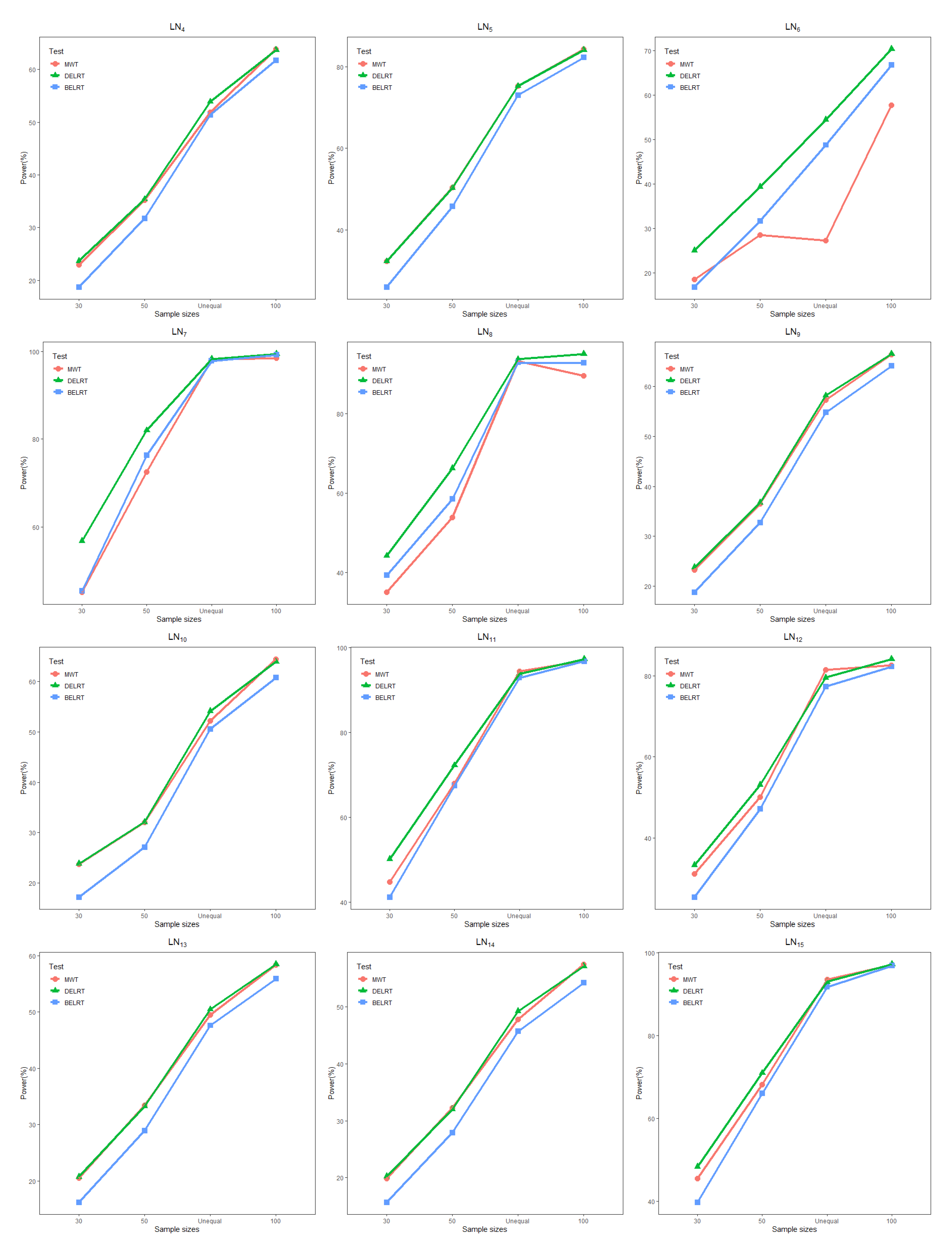
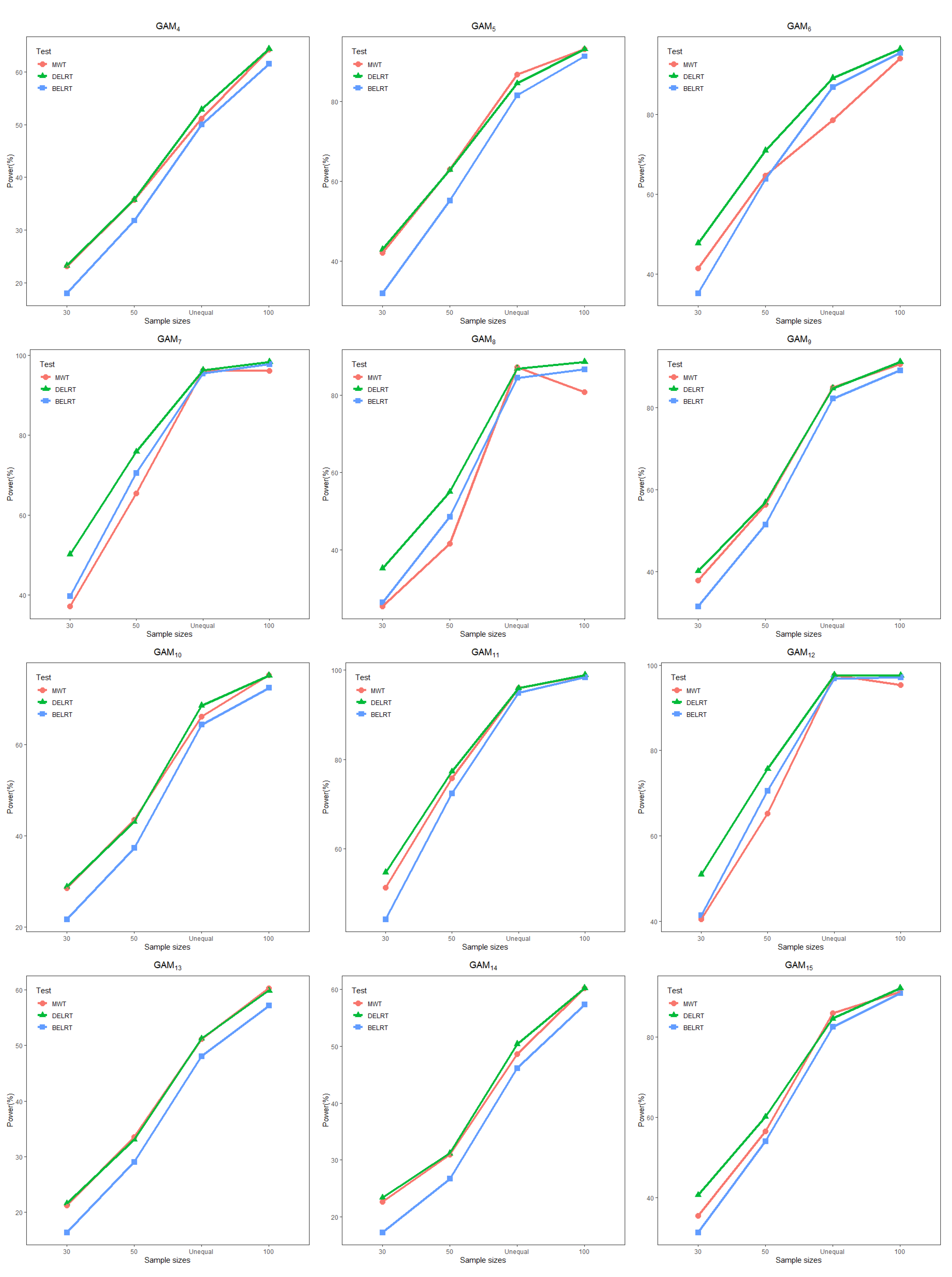
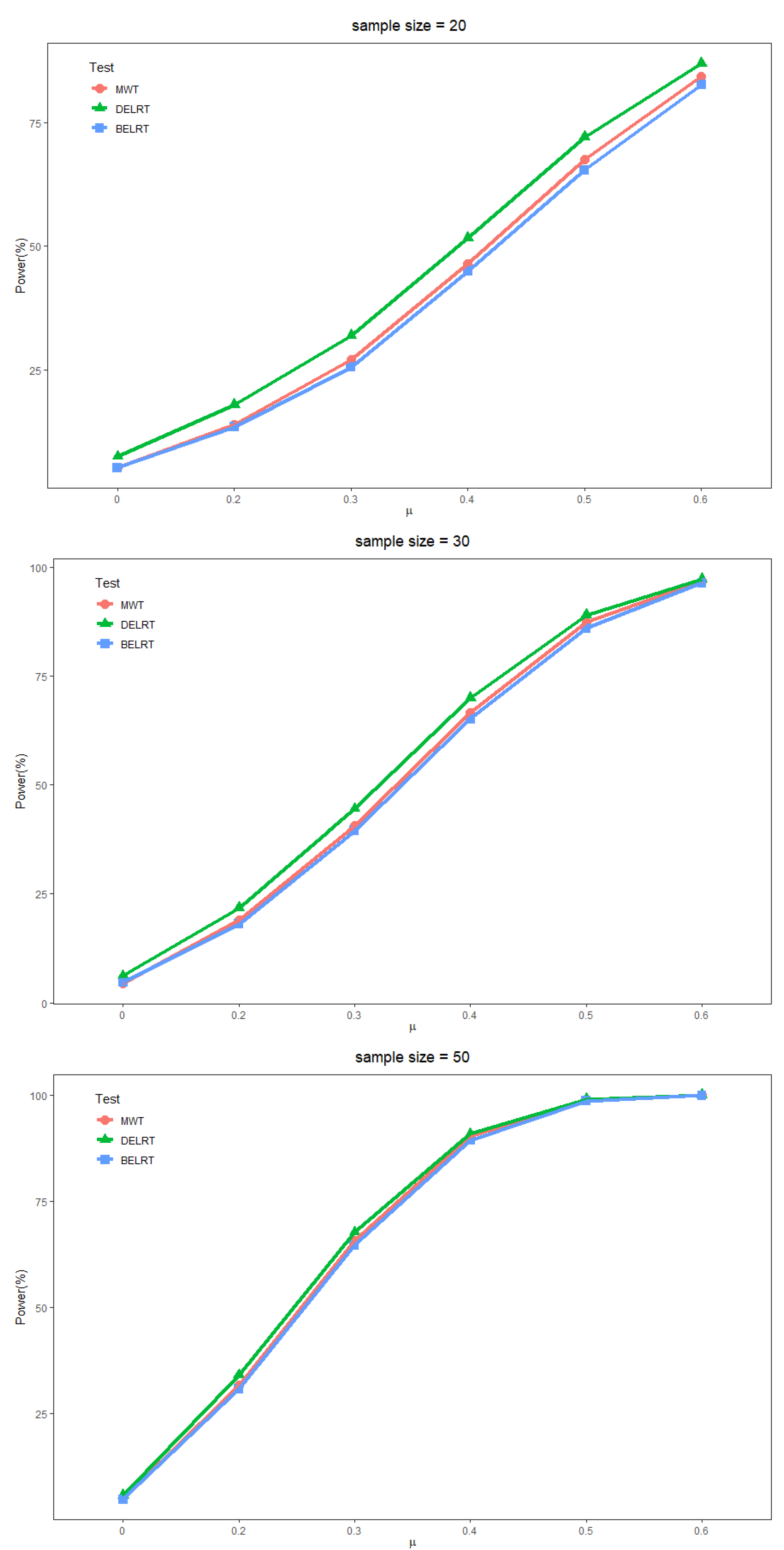
In our simulations we make comparison between three tests. In addition to the modified Wald test we proposed, denoted by “MWT”, the others are the dual empirical likelihood ratio test proposed by Cai et al. [9] and the empirical likelihood ratio test using the bootstrap procedure proposed by Wang et al. [15], which are denoted by “DELRT” and “BELRT”, respectively. We hope to show that our modified Wald test is available for different cases. In the first simulation study, we illustrate the case when the number of populations is large. We compare the performances and computational costs of the three tests. It can be seen that MWT controls the type-I error better than DELRT while taking much less time than BELRT. In the second one, we look into three normal distributions with the same scale and study how the tests perform with the change in location parameter. This means that the three populations vary from the same to totally different. We can clearly see from Figure 1 how the three tests perform. In the third simulation study we hope to verify Remark 3 in our context, which shows an interesting phenomenon of the power effected by sample sizes under certain alternative hypotheses. In the last one, we consider the semicontinuous case when the continuous part is either log-normal or a gamma distribution. The same parameter settings are also considered by Wang et al. [15]. From Figure 2 and Figure 3, we can show that our method is competitive.

4.1. Scenario 1

We consider the DRM when $(m+1)=2,3,5,8$, and 11. Let $G_0$ be the standard normal distribution while the rest are the normal distribution with scale fixed to 1 and location fixed to $\mu$. We consider the cases when $\mu =0,0.5,0.75,1$. We choose the same sample size $n_0=n_1=\cdots =n_m=30$ and 50 for all the populations and generate $M=1000$ repetitions for each situation with different m and $\mu$. Then, we calculate the type-I error of the three statistics when $\mu =0$ and the power of them when $\mu \ne 0$ at the 5% significance level. The results are shown in Table 1 and Table 2, respectively.

Table 1. Type-I error and power of the three test statistics for different $(m+1)=2,3,5,8,11$ and $\mu =0,0.5,0.75,1$ when the sample size is 30.

$(\mathit{m}+1)$	$\mathit{\mu }$	MWT	DELRT	BELRT
2	0	5.6	6.7	4.8
	0.5	39.7	40.8	34.1
	0.75	73.7	74.3	69.5
	1	93.8	93.8	92.6
3	0	4.9	6.0	4.7
	0.5	35.6	43.1	38.1
	0.75	71.8	79.1	76.1
	1	94.0	96.8	95.0
5	0	5.7	8.0	5.4
	0.5	32.1	39.2	32.7
	0.75	68.3	75.3	70.8
	1	93.2	95.4	93.9
8	0	6.0	8.8	5.9
	0.5	30.0	37.3	30.3
	0.75	65.3	72.5	66.2
	1	93.3	94.5	93.0
11	0	5.6	7.4	4.6
	0.5	26.5	31.5	25.4
	0.75	59.7	65.3	58.2
	1	89.2	91.8	88.3

Table 2. Type-I error and power of the three test statistics for different $(m+1)=2,3,5,8,11$ and $\mu =0,0.5,0.75,1$ when the sample size is 50.

$(\mathit{m}+1)$	$\mathit{\mu }$	MWT	DELRT	BELRT
2	0	5.4	6.1	5.1
	0.5	59.6	60.3	57.4
	0.75	92.8	92.8	92.5
	1	99.6	99.6	99.3
3	0	4.9	5.9	4.7
	0.5	60.0	65.1	61.9
	0.75	94.0	95.6	95.0
	1	99.4	99.5	99.5
5	0	5.5	7.1	5.8
	0.5	56.2	59.6	56.3
	0.75	93.7	95.1	94.1
	1	100.0	100.0	100.0
8	0	5.8	6.8	5.5
	0.5	49.7	53.9	49.2
	0.75	90.9	92.3	90.3
	1	99.7	99.8	99.8
11	0	5.1	6.1	5.2
	0.5	48.9	51.7	49.8
	0.75	90.2	90.3	90.2
	1	99.6	99.8	99.7

It can be seen that the type-I error of DELRT is not as well controlled as the other two. The type-I error and the power of MWT is similar to that of BELRT. However, the computational cost of MWT is much smaller. For the DELRT and the modified Wald test, realizing a repetition of $M=1000$ when $(m+1)=11$ needs no more than 40 s. However, for the bootstrap procedure when $B=999$, it takes nearly 4 h using the “for” loop in the R programming language to realize a single repetition of $M=1000$ when $(m+1)=5$ and 12 h when $(m+1)=8$. When it comes to $(m+1)=11$, it took nearly a whole day. Certainly we can use some parallel computational methods to accelerate the computation, but the running time is still a big challenge. The modified Wald test statistic we proposed seems to be a promising compromise, especially when the number of the population is large. It controls the type-I error better than DELRT while retaining a similar computational cost.

4.2. Scenario 2

In the second simulation study, we show how our test statistic performs in the case of three continuous populations. We choose the three populations as normal distributions with the scale equal to 1. The location parameters of the three are set to be $-\mu$, 0, and $\mu$. Then, we change $\mu$ from 0.2 to $0.6$ to see how our test statistic performs when the three distributions vary from “similar” to “totally different”. We consider the case with equal sample sizes $n_i=20,30$, and 50, $i=0,1,2$. For each sample size, we consider $\mu =0,0.3,0.4,0.5$, and $0.6$. We generate M = 10,000 repetitions for each case and show the comparison of the three statistics in Table 3 and Figure 1. In this figure, “MWT”, “DELRT”, and “BELRT” denote the modified Wald test, dual empirical likelihood ratio test, and bootstrap empirical likelihood ratio test, respectively.

Table 3. Type-I error and the power of the three statistics in the case of three populations.

${\mathit{n}}_{\mathit{i}}$	$\mathit{\mu }$	MWT	DELRT	BELRT
20	0	5.15	7.42	5.12
	0.2	13.84	17.90	13.39
	0.3	27.08	31.90	25.5
	0.4	46.37	51.67	44.87
	0.5	67.50	72.07	65.42
	0.6	84.34	86.99	82.67
30	0	4.39	6.19	4.65
	0.2	18.93	21.80	18.06
	0.3	40.63	44.49	39.44
	0.4	66.60	69.93	65.1
	0.5	87.29	89.03	85.94
	0.6	96.78	97.24	96.36
50	0	4.80	5.77	4.80
	0.2	31.63	34.02	30.81
	0.3	65.69	67.68	64.62
	0.4	90.18	90.77	89.30
	0.5	98.73	98.92	98.59
	0.6	99.96	99.96	99.81

Figure 1. Type-I error and power (%) of the three statistics in simulation two for different sample sizes.

It can be seen that the modified Wald test can control the type-I error nicely in this case, even when the sample size is small. The power of the Wald test is always smaller than that of the DELRT due to the better control of the type-I error. However, the disparity is gradually eliminated with the increase in the sample size and the differences between the populations.

4.3. Scenario 3

In this simulation study, we verify the conclusion in Remark 3. The total sample size n is fixed and $m=2$ and 4 are under consideration. We choose different $(n_0,n_1,\cdots ,n_m)$ for both cases and compare the power for different sample sizes. We fixed $g_0$ to $N(0,1)$, $LN(0,1)$, and $GAM(1,2)$. The rest $g_1=\cdots =g_m$ are chosen to be the same distribution corresponding to $g_0$ with different $\mu =0.3,0.5$, and 0.7 for normal and log-normal cases and $1.2,1.4$, and 1.6 for the location parameter in gamma’s case. For each different sample size and $\mu$, we generalize M = 100,000 repetitions and calculate the power. The details are given in Table 4 and Table 5. The symbols I to VIII in Table 5 denote different sample sizes which are shown in Table 6.

Table 4. The power of testing $H_0$ at significance level 0.05 for different sample sizes and $\mu$ when $m=2$.

	$\mathit{\mu }$	$({\mathit{n}}_0,{\mathit{n}}_1,{\mathit{n}}_2)$
		(40, 40, 120)	(40, 80, 80)	(60, 40, 100)	(60, 70, 70)	(100, 50, 50)	(140, 30, 30)	(180, 10, 10)
	0.3	19.23	20.83	26.76	27.86	34.00	29.65	16.58
Normal	0.5	51.96	55.04	68.84	70.21	80.04	72.47	37.92
	0.7	85.15	87.23	95.22	95.80	98.42	96.27	66.09
	0.3	24.38	24.46	30.81	30.85	36.20	31.08	17.17
Log-normal	0.5	61.29	61.30	73.95	73.86	81.91	74.01	38.99
	0.7	90.65	90.74	96.73	96.81	98.67	96.66	67.21
	1.2	18.53	18.67	21.52	21.55	46.09	36.02	16.05
Gamma	1.4	55.67	55.82	66.28	66.36	88.58	78.41	35.41
	1.6	87.12	87.24	94.19	94.19	99.26	97.12	59.99

Table 5. The power of testing $H_0$ at significance level 0.05 for different sample sizes and $\mu$ when $m=4$.

	$\mathit{\mu }$	$({\mathit{n}}_0,{\mathit{n}}_1,{\mathit{n}}_2,{\mathit{n}}_3,{\mathit{n}}_4)$
		Case I	Case II	Case III	Case IV	Case V	Case VI	Case VII	Case VIII
	0.3	10.65	10.33	16.22	24.32	25.90	25.56	25.59	20.31
Normal	0.5	23.44	22.81	43.76	65.58	68.34	67.84	66.68	49.41
	0.7	45.98	44.53	77.86	94.56	95.61	95.48	94.84	81.69
	0.3	13.27	13.21	19.13	26.96	28.31	28.20	27.61	21.64
Log-normal	0.5	30.24	30.39	49.77	69.18	71.25	71.19	69.33	51.45
	0.7	57.14	57.25	83.11	95.73	96.42	96.35	95.62	83.18
	1.2	11.87	11.72	14.46	17.12	16.56	16.65	15.57	12.31
Gamma	1.4	29.88	29.87	44.65	57.26	57.01	56.72	52.65	32.89
	1.6	56.63	56.52	78.95	91.10	91.22	91.28	88.34	64.47

Table 6. The different settings of $(n_0,n_1,n_2,n_3,n_4)$ in Table 5.

Case Label	Sample Size
I	(20, 30, 40, 50, 60)
II	(20, 45, 45, 45, 45)
III	(40, 40, 40, 40, 40)
IV	(80, 30, 30, 30, 30)
V	(100, 25, 25, 25, 25)
VI	(100, 40, 30, 20, 10)
VII	(120, 20, 20, 20, 20)
VIII	(160, 10, 10, 10, 10)

It can be seen that the conclusion in Remark 3 holds basically. It is obviously that $n_0$ has the biggest impact on the power while the rest of the sample sizes $n_1,\cdots ,n_m$ do not seem to have much influence. This can be seen quite clearly from the comparison of the first four sample sizes in the three-sample case and case I and II, and case V and VI in the five-sample case.

4.4. Scenario 4

In this simulation study, we consider the semicontinuous case. We adopt the same parameter settings as in Wang et al. [15]. Assume that the samples are generated from

$$F_i\left(x\right)=p_{i}I(x=0)+(1-p_i)I(x>0)G_i\left(x\right),$$

for $i=0,1,2$, where $G_i$’s are all log-normal or gamma distributions. The parameters of $F_i$ are present in Table 7. Each of LN${}_1$–LN${}_{15}$ and GAM${}_1$–GAM${}_{15}$ in the first column denotes a mixture model whose continuous part follows a log-normal or gamma distribution. $p_i$ denotes the probability of drawing a zero observation for $F_i$. LN$(a_i,b_i)$ denotes a log-normal distribution whose associated normal distribution has the mean $a_i$ and variance $b_i$. GAM$(a_i,b_i)$ denotes a gamma distribution with shape parameter $a_i$ and scale parameter $b_i$. We consider both the equal sample sizes where $n_0=n_1=n_2=30,50,100$ and the unequal sample size where $(n_0,n_1,n_2)=(50,100,150)$. For every parameter setting, we generate M = 10,000 repetitions. We calculate the type-I error of testing homogeneity at 5% significance level for LN${}_1$–LN${}_3$ and GAM${}_1$–GAM${}_3$, and the power of that for the rest of the parameter settings. The type-I errors of the three statistics are shown in Table 8 while the powers are shown in Table 9 and Table 10, respectively, for the log-normal and the gamma cases. To have a better view of them, we show the powers of the three statistics in Figure 2 and Figure 3. It can be seen that the results are competitive.

Table 7. Parameter settings for simulation study 3.

Model	$({\mathit{p}}_0,{\mathit{p}}_1,{\mathit{p}}_2)$	$({\mathit{a}}_0,{\mathit{a}}_1,{\mathit{a}}_2)$	$({\mathit{b}}_0,{\mathit{b}}_1,{\mathit{b}}_2)$	Mean	Variance
LN${}_1$	(0.2, 0.2, 0.2)	(0.0, 0.0, 0.0)	(1.0, 1.0,1.0)	(1.32, 1.32, 1.32)	(4.17, 4.17, 4.17)
LN${}_2$	(0.4, 0.4, 0.4)	(0.0, 0.0, 0.0)	(1.0, 1.0, 1.0)	(0.99, 0.99, 0.99)	(3.45,3.45,3.45)
LN${}_3$	(0.7, 0.7, 0.7)	(0.0, 0.0, 0.0)	(1.0, 1.0, 1.0)	(0.49, 0.49, 0.49)	(1.97, 1.97, 1.97)
LN${}_4$	(0.2, 0.3, 0.4)	(0.0, 0.0, 0.0)	(1.0, 1.0, 1.0)	(1.32, 1.15, 0.99)	(4.17, 3.84, 3.45)
LN${}_5$	(0.4, 0.4, 0.4)	(0.0, 0.5, 1.0)	(2.0, 2.0, 2.0)	(1.63, 2.69, 4.43)	(30.10, 81.82, 222.40)
LN${}_6$	(0.6, 0.6, 0.6)	(0.0, 0.0, 0.0)	(1.0, 2.0, 3.0)	(0.66, 1.09, 1.79)	(2.52, 20.66, 158.16)
LN${}_7$	(0.5, 0.6, 0.7)	(0.0, 0.5, 1.0)	(3.0, 2.0, 1.0)	(2.24, 1.79, 1.34)	(196.69, 56.15, 14.57)
LN${}_8$	(0.6, 0.6, 0.6)	(0.0, 0.5, 1.0)	(3.0, 2.0, 1.0)	(1.79, 1.79, 1.79)	(158.16, 56.15, 18.63)
LN${}_9$	(0.3, 0.4, 0.5)	(0.0, 0.15, 0.34)	(2.0, 2.0, 2.0)	(1.90, 1.90, 1.90)	(34.60, 40.97, 49.89)
LN${}_{10}$	(0.4, 0.5, 0.6)	(0.0, 0.0, 0.0)	(2.0, 2.36, 2.81)	(1.63, 1.63, 1.63)	(30.10, 53.95, 107.90)
LN${}_{11}$	(0.4, 0.5, 0.6)	(0.0, 0.5, 1.0)	(2.69, 2.05, 1.5)	(2.30, 2.30, 2.30)	(124.67, 77.32, 54.07)
LN${}_{12}$	(0.5, 0.5, 0.5)	(0.0, 0.5, 1.0)	(2.46, 1.98, 1.5)	(1.71, 2.21, 2.88)	(65.93, 65.93, 65.93)
LN${}_{13}$	(0.3, 0.4, 0.5)	(0.0, 0.07, 0.15)	(2.0, 2.0, 2.0)	(1.90, 1.75, 1.58)	(34.60, 34.60, 34.60)
LN${}_{14}$	(0.3, 0.4, 0.5)	(0.0, 0.0, 0.0)	(2.0, 2.07, 2.15)	(1.90, 1.69, 1.46)	(34.60, 34.60, 34.60)
LN${}_{15}$	(0.4, 0.5, 0.6)	(0.0, 0.5, 1.0)	(2.28, 1.88, 1.5)	(1.88, 2.11, 2.30)	(54.07, 54.07, 54.07)
GAM${}_1$	(0.2, 0.2, 0.2)	(1.0, 1.0, 1.0)	(1.0, 1.0, 1.0)	(0.8, 0.8, 0.8)	(0.96, 0.96, 0.96)
GAM${}_2$	(0.4, 0.4, 0.4)	(1.0, 1.0, 1.0)	(1.0, 1.0, 1.0)	(0.6, 0.6, 0.6)	(0.84, 0.84, 0.84)
GAM${}_3$	(0.7, 0.7, 0.7)	(1.0, 1.0, 1.0)	(1.0, 1.0, 1.0)	(0.3, 0.3, 0.3)	(0.51, 0.51, 0.51)
GAM${}_4$	(0.2, 0.3, 0.4)	(1.0, 1.0, 1.0)	(2.0, 2.0, 2.0)	(1.6, 1.4, 1.2)	(3.84, 3.64, 3.36)
GAM${}_5$	(0.6, 0.6, 0.6)	(1.0, 1.5, 2.0)	(2.0, 2.0, 2.0)	(0.8, 1.2, 1.6)	(2.56, 4.56, 7.04)
GAM${}_6$	(0.6, 0.6, 0.6)	(1.0, 1.0, 1.0)	(1.0, 2.0, 3.0)	(0.4, 0.8, 1.2)	(0.64, 2.56, 5.76)
GAM${}_7$	(0.4, 0.5, 0.6)	(1.0, 1.5, 3.0)	(3.0, 2.0, 1.0)	(1.8, 1.5, 1.2)	(7.56, 5.25, 3.36)
GAM${}_8$	(0.5, 0.5, 0.5)	(1.0, 1.5, 3.0)	(3.0, 2.0, 1.0)	(1.5, 1.5, 1.5)	(6.75, 5.25, 3.75)
GAM${}_9$	(0.4, 0.5, 0.6)	(1.5, 1.8, 2.25)	(2.0, 2.0, 2.0)	(1.8, 1.8, 1.8)	(5.76, 6.84, 8.46)
GAM${}_{10}$	(0.4, 0.5, 0.6)	(1.0, 1.0, 1.0)	(2.0, 2.4, 3.0)	(1.2, 1.2, 1.2)	(3.36, 4.32, 5.76)
GAM${}_{11}$	(0.4, 0.5, 0.6)	(2.0, 3.0, 4.0)	(2.0, 1.6, 1.5)	(2.4, 2.4, 2.4)	(8.64, 9.60, 12.24)
GAM${}_{12}$	(0.4, 0.4, 0.4)	(1.0, 1.5, 3.0)	(2.0, 1.53, 0.92)	(1.20, 1.37, 1.66)	(3.36, 3.36, 3.36)
GAM${}_{13}$	(0.3, 0.4, 0.5)	(1.5, 1.56, 1.66)	(2.0, 2.0, 2.0)	(2.1, 1.87, 1.66)	(6.09, 6.09, 6.09)
GAM${}_{14}$	(0.3, 0.4, 0.5)	(1.0, 1.0, 1.0)	(2.0, 2.08, 2.20)	(1.4, 1.25, 1.1)	(3.64, 3.64, 3.64)
GAM${}_{15}$	(0.4, 0.5, 0.6)	(2.0, 3.0, 4.0)	(2.0, 1.52, 1.26)	(2.4, 2.28, 2.02)	(8.64, 8.64, 8.64)

Table 8. Type I error rates (%) for testing $H_0$ at significance level 0.05 when data are generated from LN${}_1$–LN${}_3$ and GAM${}_1$–GAM${}_3$ in Table 7.

	30			50			Unequal			100
	MWT	DELRT	BELRT	MWT	DELRT	BELRT	MWT	DELRT	BELRT	MWT	DELRT	BELRT
LN${}_1$	6.27	7.28	5.16	6.12	6.54	5.53	5.67	5.80	5.20	5.81	6.39	5.68
LN${}_2$	6.29	7.41	4.78	5.59	6.42	4.83	4.94	5.82	4.92	5.88	6.24	5.31
LN${}_3$	7.32	9.75	4.16	6.92	8.35	5.34	5.98	7.11	5.38	5.05	5.78	4.40
GAM${}_1$	5.95	7.44	5.08	4.98	5.97	4.72	4.96	5.03	3.91	5.58	5.77	4.83
GAM${}_2$	6.67	7.54	5.20	6.31	7.21	5.32	5.46	6.04	4.91	5.03	5.82	4.72
GAM${}_3$	8.72	11.04	5.97	7.30	9.23	5.61	5.56	6.86	4.99	5.20	6.57	4.85

Table 9. Power (%) for testing $H_0$ at significance level 0.05 when data are generated from LN${}_4$–LN${}_{15}$ in Table 7.

	30			50			Unequal			100
	MWT	DELRT	BELRT	MWT	DELRT	BELRT	MWT	DELRT	BELRT	MWT	DELRT	BELRT
LN${}_4$	22.91	23.66	18.68	35.22	35.37	31.73	51.89	53.87	51.36	63.90	63.68	61.71
LN${}_5$	32.29	32.26	25.89	50.33	50.21	45.66	75.33	75.26	73.04	84.40	84.13	82.28
LN${}_6$	18.47	25.03	16.72	28.54	39.30	31.63	27.23	54.44	48.74	57.68	70.41	66.76
LN${}_7$	45.04	56.76	45.37	72.55	81.95	76.22	98.12	98.27	97.78	98.51	99.44	99.19
LN${}_8$	34.93	44.15	39.24	53.91	66.28	58.47	93.30	93.76	92.88	89.52	95.09	92.78
LN${}_9$	23.22	23.78	18.77	36.54	36.77	32.73	57.24	58.15	54.75	66.41	66.52	64.08
LN${}_{10}$	23.77	23.84	17.19	32.05	32.11	27.12	52.13	54.09	50.54	64.43	63.87	60.69
LN${}_{11}$	44.82	50.17	41.15	67.94	72.27	67.43	94.42	93.83	92.89	96.92	97.33	96.78
LN${}_{12}$	31.07	33.24	25.34	50.02	53.10	47.09	81.51	79.53	77.33	82.64	84.13	82.21
LN${}_{13}$	20.49	20.75	16.18	33.44	33.25	28.94	49.47	50.48	47.62	58.35	58.52	55.89
LN${}_{14}$	19.90	20.23	15.67	32.29	32.01	27.88	47.76	49.19	45.65	57.45	57.09	54.16
LN${}_{15}$	45.51	48.36	39.74	68.15	70.96	66.04	93.49	93.00	91.77	97.08	97.25	96.89

Table 10. Power (%) for testing $H_0$ at significance level 0.05 when data are generated from GAM${}_4$–GAM${}_{15}$ in Table 7.

	30			50			Unequal			100
	MWT	DELRT	BELRT	MWT	DELRT	BELRT	MWT	DELRT	BELRT	MWT	DELRT	BELRT
GAM${}_4$	23.17	23.32	18.02	35.76	35.79	31.80	51.19	52.87	49.98	64.18	64.34	61.47
GAM${}_5$	42.16	42.98	31.96	63.01	62.84	55.18	86.68	84.47	81.51	93.11	93.02	91.24
GAM${}_6$	41.39	47.65	35.12	64.66	70.92	63.75	78.57	89.12	86.83	93.95	96.40	95.42
GAM${}_7$	37.03	50.11	39.61	65.48	75.81	70.48	96.23	96.32	95.46	96.14	98.40	97.77
GAM${}_8$	25.23	35.12	26.26	41.51	55.00	48.53	87.33	86.97	84.52	80.90	88.72	86.75
GAM${}_9$	37.85	40.10	31.44	56.27	56.90	51.48	84.96	84.73	82.20	90.60	91.21	89.09
GAM${}_{10}$	28.49	28.87	21.69	43.46	43.07	37.32	66.08	68.49	64.31	75.19	75.05	72.36
GAM${}_{11}$	51.40	54.77	44.25	75.78	77.28	72.37	95.87	95.92	94.85	98.69	98.87	98.32
GAM${}_{12}$	40.43	50.95	41.38	65.29	75.65	70.52	97.69	97.68	96.80	95.33	97.57	97.10
GAM${}_{13}$	21.23	21.61	16.36	33.55	33.07	29.02	51.13	51.24	48.06	60.32	59.87	57.14
GAM${}_{14}$	22.63	23.39	17.25	30.91	31.20	26.68	48.67	50.40	46.13	60.22	60.24	57.32
GAM${}_{15}$	35.56	40.67	31.36	56.55	60.12	54.06	85.90	84.53	82.44	91.19	92.12	90.77

Figure 2. Power (%) for testing $H_0$ at significance level 0.05 when data are generated from LN${}_4$–LN${}_{15}$ in Table 7.

Figure 3. Power (%) for testing $H_0$ at significance level 0.05 when data are generated from GAM${}_4$–GAM${}_{15}$ in Table 7.

5. Real Data Sample

In this section, we employ the real data example suggested by Wang et al. [15] which is available from the website of the University of Waterloo weather station data archive (http://weather.uwaterloo.ca/data.html, accessed on 1 June 2023). We focus on the data that records the daily precipitation measurements (in millimeters) in the North Campus of the University of Waterloo, Canada and investigate whether the precipitation distribution has changed over the past few years.

Benefiting from what Wang et al. [15] has previously reported, to reduce the time dependence among the observations, we take every fourth measurement into our analysis, i.e., only use the observations on days 1, 5, 9, …, 361, which gives a sample size of 91 for each sample. Then, we consider two cases, one is from 2003 to 2006 and the other from 2008 to 2012, we hope to obtain some information about the changing of the precipitation distribution in the last few years. Some summaries of the samples are given below

• From 2003 to 2006, the estimates of the probability of dry days are (0.30, 0.40, 0.42, 0.42) while those of 2008 to 2012 are (0.45, 0.49, 0.43, 0.38, 0.40).
• The sample means of 2003 to 2006 are (2.05, 3.54, 3.40, 3.50) while those of 2008 to 2012 are (3.42, 1.37, 2.29, 4.08, 3.09).
• The sample variances are (17.52, 41.07, 76.10, 59.50) and (95.19, 13.53, 18.35, 73.83, 59.76), respectively.

For each null and alternative hypothesis, we fit the data to both the log-normal and the gamma mixture under the assumption of the density ratio model using the maximum likelihood estimate. The details are give in Table 11 below. There is a small difference between the parameters of ours and Wang et al. [15], this may be caused by the mistake when summarizing the data of the year 2003. LN${}_{16}$ and GAM${}_{16}$ are the parameters under the null hypothesis of the case of 2003 to 2006, while LN${}_{18}$ and GAM${}_{18}$ are those of 2008 to 2012. The rest of the parameters are for the alternative hypotheses.

Table 11. The parameter settings for the null and alternative hypothesis for testing homogeneity.

Model	p	a	b	Mean	Variance
LN${}_{16}$	(0.38, 0.38, 0.38, 0.38)	(0.49, 0.49, 0.49, 0.49)	(2.58, 2.58, 2.58, 2.58)	(3.67, 3.67, 3.67, 3.67)	(274.43, 274.43, 274.43, 274.43)
LN${}_{17}$	(0.30, 0.40, 0.42, 0.42)	(0.10, 1.05 0.36, 0.52)	(2.13, 1.70, 3.08, 3.00)	(2.25, 4.04, 3.91, 4.39)	(55.77, 131.52, 559.29, 645.92)
LN${}_{18}$	(0.43, 0.43, 0.43, 0.43, 0.43)	(0.43, 0.43, 0.43, 0.43, 0.43)	(2.66, 2.66, 2.66, 2.66, 2.66)	(3.29, 3.29, 3.29, 3.29, 3.29)	(262.59, 262.59, 262.59, 262.59, 262.59)
LN${}_{19}$	(0.45, 0.49, 0.43, 0.38, 0.40)	(0.66, 0.04, 0.32, 0.57, 0.48)	(2.37, 2.03, 2.78, 3.26, 2.54)	(3.48, 1.46, 3.15, 5.54, 3.47)	(222.47, 29.97, 271.27, 1266.19, 238.72)
GAM${}_{16}$	(0.38, 0.38, 0.38, 0.38)	(0.55, 0.55, 0.55, 0.55)	(9.11, 9.11, 9.11, 9.11)	(3.12, 3.12, 3.12, 3.12)	(34.44, 34.44, 34.44, 34.44)
GAM${}_{17}$	(0.30, 0.40, 0.42, 0.42)	(0.63, 0.82, 0.46, 0.50)	(4.61, 7.12, 12.70, 12.05)	(2.05, 3.54, 3.40, 3.50)	(11.21, 33.40, 51.42, 50.92)
GAM${}_{18}$	(0.43, 0.43, 0.43, 0.43, 0.43)	(0.53, 0.53, 0.53, 0.53, 0.53)	(9.33, 9.33, 9.33, 9.33, 9.33)	(2.83, 2.83, 2.83, 2.83, 2.83)	(32.44, 32.44, 32.44, 32.44, 32.44)
GAM${}_{19}$	(0.45, 0.49, 0.43, 0.38, 0.40)	(0.55, 0.64, 0.58, 0.48, 0.54)	(10.97, 4.24, 6.90, 13.74, 9.40)	(3.32, 1.37, 2.29, 4.08, 3.09)	(45.46, 7.65, 19.69, 66.45, 35.28)

We apply the modified Wald test on the null hypotheses LN${}_{16}$ and GAM${}_{16}$, respectively. The test statistic is 21.65 for the log-normal mixture and 24.02 for the gamma mixture. Both statistics are larger than the 0.05% quantile of ${\chi }_8^2$, which is 15.51. The null hypothesis should be rejected at the significance level 0.05. We then move on to the case of 5 years. This time the result becomes quite different. The test statistic for LN${}_{18}$ is 11.70, while that for GAM${}_{18}$ is 9.95, this is smaller than the 0.05% quantile of ${\chi }_{10}^2$, which is 18.3074, which means that the null hypothesis is true at the significance level 0.05. The two simulations above indicate that the precipitation distribution of the area was changing from 2003 to 2006, but may have remained unchanged over 2008 to 2012.

6. Conclusions

In this paper, we propose a modified Wald test for homogeneity of the density ratio model. Since the density functions are unknown, recent works mainly focus on the empirical likelihood ratio test, which is a nonparametric method. We transform the problem of testing homogeneity to testing the equalities of the mean parameters of the exponential family of distributions. Then, we propose a modified Wald test, which is a parametric method. The simulations show that the type-I error of the modified Wald test is smaller than that of the empirical likelihood ratio test. Since the modified Wald test statistic converges in distribution to the ${\chi }^2$ distribution, it can further be applied to the semicontinuous data. It should be noticed that for the DRM, we test hypotheses ${\beta }_1={\beta }_2=\cdots ={\beta }_m=0$. This can be generalized to test hypotheses ${\beta }_1={\beta }_{10},{\beta }_2={\beta }_{20},\cdots ,{\beta }_m={\beta }_{m0}$.

References

- Anderson, J.A. Multivariate logistic compounds. Biometrika 1979, 66, 17–26. [Google Scholar] [CrossRef]
- Qin, J.; Zhang, B. A goodness-of-fit test for logistic regression models based on case-control data. Biometrika 1997, 84, 609–618. [Google Scholar] [CrossRef]
- Zhang, B. Assessing goodness-of-fit of generalized logit models based on case-control data. J. Multivar. Anal. 2002, 82, 17–38. [Google Scholar] [CrossRef]
- Qin, J. Empirical likelihood ratio based confidence intervals for mixture proportions. Ann. Stat. 1999, 27, 1368–1384. [Google Scholar] [CrossRef]
- Zou, F.; Fine, J.P.; Yandell, B.S. On empirical likelihood for a semiparametric mixture model. Biometrika 2002, 89, 61–75. [Google Scholar] [CrossRef][Green Version]
- Zhang, B. Quantile estimation under a two-sample semi-parametric model. Bernoulli 2000, 6, 491–511. [Google Scholar] [CrossRef]
- Chen, J.; Liu, Y. Quantile and quantile-function estimations under density ratio model. Ann. Stat. 2013, 41, 1669–1692. [Google Scholar] [CrossRef]
- Fokianos, K.; Kedem, B.; Qin, J.; Short, D.A. A semiparametric approach to the one-way layout. Technometrics 2001, 43, 56–65. [Google Scholar] [CrossRef]
- Cai, S.; Chen, J.; Zidek, J.V. Hypothesis testing in the presence of multiple samples under density ratio models. Statist. Sin. 2017, 27, 761–783. [Google Scholar] [CrossRef]
- Patil, G.P.; Rao, C.R. Weighted Distributions and Size-Biased Sampling with Applications to Wildlife Populations and Human Families. Biometrics 1978, 34, 179–189. [Google Scholar] [CrossRef]
- Rao, C.R. Weighted Distributions Arising Out of Methods of Ascertainment: What Population Does a Sample Represent? In A Celebration of Statistics; Springer: New York, NY, USA, 1985; pp. 543–569. [Google Scholar]
- Rao, C.R. On Discrete Distributions Arising out of Methods of Ascertainment. Sankhyā Indian J. Stat. Ser. A 1965, 27, 311–324. [Google Scholar]
- Lele, S.R.; Keim, J.L. Weighted distributions and estimation of resource selection probability functions. Ecology 2006, 87, 3021–3028. [Google Scholar] [CrossRef]
- Qin, J.; Lawless, J. Empirical likelihood and general estimating equations. Ann. Stat. 1994, 22, 300–325. [Google Scholar] [CrossRef]
- Wang, C.; Marriott, P.; Li, P. Testing homogeneity for multiple nonnegative distributions with excess zero observations. Comput. Stat. Data Anal. 2017, 114, 146–157. [Google Scholar] [CrossRef]
- Tu, W.; Zhou, X.H. A Wald test comparing medical costs based on log-normal distributions with zero valued costs. Stat. Med. 1999, 18, 2749–2761. [Google Scholar] [CrossRef]
- Muralidharan, K.; Kale, B.K. Modified Gamma distribution with singularity at zero. Commun. Stat.-Simul. Comput. 2002, 31, 143–158. [Google Scholar] [CrossRef]
- Kassahun-Yimer, W.; Albert, P.S.; Lipsky, L.M.; Nansel, T.R.; Liu, A. A joint model for multivariate hierarchical semicontinuous data with replications. Stat. Methods Med. Res. 2019, 28, 858–870. [Google Scholar] [CrossRef]
- Neelon, B.; O’Malley, A.J.; Smith, V.A. Modeling zero-modified count and semicontinuous data in health services research part 1: Background and overview. Stat. Med. 2016, 35, 5070–5093. [Google Scholar] [CrossRef]
- Neelon, B.; O’Malley, A.J.; Smith, V.A. Modeling zero-modified count and semicontinuous data in health services research part 2: Case studies. Stat. Med. 2016, 35, 5094–5112. [Google Scholar] [CrossRef]
- Lachenbruch, P.A. Analysis of data with excess zeros. Stat. Methods Med. Res. 2002, 11, 297–302. [Google Scholar] [CrossRef]
- Su, L.; Tom, B.D.M.; Farewell, V.T. Bias in 2-part mixed models for longitudinal semicontinuous data. Biostatistics 2009, 10, 374–389. [Google Scholar] [CrossRef]
- Smith, V.A.; Preisser, J.S.; Neelon, B.; Maciejewski, M.L. A marginalized two-part model for semicontinuous data. Stat. Med. 2014, 33, 4891–4903. [Google Scholar] [CrossRef] [PubMed]
- Wang, C.; Tu, D. A bootstrap semiparametric homogeneity test for the distributions of multigroup proportional data, with applications to analysis of quality of life outcomes in clinical trials. Stat. Med. 2020, 39, 1715–1731. [Google Scholar] [CrossRef]
- Wilcox, R.R. ANOVA: A Paradigm for Low Power and Misleading Measures of Effect Size? Rev. Educ. Res. 1995, 65, 51–77. [Google Scholar] [CrossRef]
- Hallstrom, A.P. A modified Wilcoxon test for non-negative distributions with a clump of zeros. Stat. Med. 2009, 29, 391–400. [Google Scholar] [CrossRef] [PubMed]
- Pauly, M.; Brunner, E.; Konietschke, F. Asymptotic permutation tests in general factorial designs. J. R. Stat. Soc. Ser. B. Stat. Methodol. 2015, 77, 461–473. [Google Scholar] [CrossRef]
Disclaimer/Publisher’s Note: The statements, opinions and data contained in all publications are solely those of the individual author(s) and contributor(s) and not of MDPI and/or the editor(s). MDPI and/or the editor(s) disclaim responsibility for any injury to people or property resulting from any ideas, methods, instructions or products referred to in the content. |
© 2023 by the authors. Licensee MDPI, Basel, Switzerland. This article is an open access article distributed under the terms and conditions of the Creative Commons Attribution (CC BY) license (https://creativecommons.org/licenses/by/4.0/).