Dynamics and Embedded Solitons of Stochastic Quadratic and Cubic Nonlinear Susceptibilities with Multiplicative White Noise in the Itô Sense

Abstract

The main purpose of this paper is to study the dynamics and embedded solitons of stochastic quadratic and cubic nonlinear susceptibilities in the Itô sense, which can further help researchers understand the propagation of soliton nonlinear systems. Firstly, a two-dimensional dynamics system and its perturbation system are obtained by using a traveling wave transformation. Secondly, the phase portraits of the two-dimensional dynamics system are plotted. Furthermore, the chaotic behavior, two-dimensional phase portraits, three-dimensional phase portraits and sensitivity of the perturbation system are analyzed via Maple software. Finally, the embedded solitons of stochastic quadratic and cubic nonlinear susceptibilities are obtained. Moreover, three-dimensional and two-dimensional solitons of stochastic quadratic and cubic nonlinear susceptibilities are plotted.

1. Introduction

The concept of an “embedded soliton” (ES) was introduced at the end of the 1990s. After that, Yang et al. [1] found ESs in a continuous model, an unstable model and a discrete model, and further explained ESs. Generally, the ES [2,3,4] is a new type of solitary wave, which exists in the continuous spectrum of a nonlinear wave system and is limited in the continuous spectrum of a nonlinear system [5,6,7]. ESs are usually used to describe the solutions of nonlinear partial differential equations from hydrodynamics, nonlinear optics and liquid crystal theory [8,9,10,11].

In recent years, the analysis of soliton solutions and the dynamic behavior of stochastic partial differential equations (SPDEs) [12,13,14,15] has greatly attracted the attention of many experts and scholars. In [12], Han et al. studied the exact solutions and bifurcation of the stochastic fractional long-short wave equation by using the dynamical system method. In [13], Zayed et al. obtained the dispersive optical solitons of the stochastic perturbed generalized Schrödinger–Hirota equation by the extended simplest equation algorithm and the ${\Phi }^6$-model expansion method. In [14], He and Wang studied the soliton solutions of the stochastic nonlinear Schrödinger equation using the bilinear method. In [15], Li and Tao derived the soliton solutions of the stochastic Benjamin–Ono equation by using the Hirota method. Based on an analysis of the above references, we find that the research results in recent years mainly focus on the discussion of soliton solutions of SPDEs. Although some papers have discussed the dynamic behavior of partial differential equations [16,17], there are few studies on the dynamic behavior, chaotic behavior and sensitivity of SPDEs and their perturbation. The main purpose of this paper is to discuss the dynamic behavior and embedded soliton solutions of a class of SPDEs and their perturbed system.

The stochastic quadratic and cubic nonlinear susceptibilities with multiplicative white noise in the Itô sense are a kind of very important SPDE, which is usually described as follows [18]

$$\left\{\begin{array}{c}i{u}_t+a_1{u}_{xx}+b_1{u}_{xt}+c_1{u}^{*}v+d_1{\left|u\right|}^{2}u+\sigma (u-i{b}_1{u}_x)\frac{dW\left(t\right)}{dt}=0,\hfill \\ i{v}_t+a_2{v}_{xx}+b_2{v}_{xt}+c_{2}v+d_2{u}^2+\delta {\left|u\right|}^{2}v+\sigma (v-i{b}_2{v}_x)\frac{dW\left(t\right)}{dt}=0,\hfill \end{array}\right.$$

(1)

where $u=u(t,x)$ and $v=v(t,x)$ are the complex-valued functions. $a_j$, $b_j$, $c_j$, $d_j$ ($j=1,2$), $\delta$ and $\sigma$ stand for real-valued constants. $a_j$ stands for the chromatic dispersion. $b_j$ stands for the spatio-temporal dispersion. $c_j$ represents the group velocity mismatch. $d_j$ is the self phase modulation. $i^2=-1$. $u^{*}$ is the complex conjugate of u. $\frac{dW\left(t\right)}{dt}$ is the white noise [19,20,21,22,23,24,25,26,27,28,29]. $W\left(t\right)$ is the standard Wiener process. $\sigma$ is the noise strength.

Here, the real-valued function of periodic perturbations $g_1$ and $g_2$ is added, which is written below:

$$\left\{\begin{array}{c}i{u}_t+a_1{u}_{xx}+b_1{u}_{xt}+c_1{u}^{*}v+d_1{\left|u\right|}^{2}u+\sigma (u-i{b}_1{u}_x)\frac{dW\left(t\right)}{dt}=g_1,\hfill \\ i{v}_t+a_2{v}_{xx}+b_2{v}_{xt}+c_{2}v+d_2{u}^2+\delta {\left|u\right|}^{2}v+\sigma (v-i{b}_2{v}_x)\frac{dW\left(t\right)}{dt}=g_2.\hfill \end{array}\right.$$

(2)

The method of planar dynamic systems was first proposed by Professor Li Jibin [30]. This method is used to construct a planar two-dimensional dynamic system and a Hamiltonian function. The dynamic characteristics of nonlinear differential equations are analyzed through phase diagrams and orbits. Recently, this method has been used by many experts and scholars to analyze the dynamic characteristics of nonlinear partial differential equations and fractional partial differential equations. This article is based on Professor Li Jibin’s plane dynamics system method to analyze the dynamic characteristics of Equation (1). By adding perturbation terms to Equation (1), this paper also takes into account the dynamic characteristics of the perturbed system. The soliton solution of Equation (1) is given by using the complete discriminant system of polynomials.

The format of this article is organized as follows: In Section 2, the dynamics of (1) and (2) are analysed. In Section 3, the embedded solitons of (1) are constructed by using the complete discrimination system method. In Section 4, the results of this article and the published results are presented in a table. In Section 5, a brief conclusion is presented.

2. Dynamics of (1) and (2)

2.1. Mathematical Derivation

Assume that the main solution of Equation (1) is as follows

$$\begin{array}{c}\hfill u(t,x)=U_1\left(\xi \right){\mathbf{e}}^{\mathbf{i}(-kx+wt+\sigma W\left(t\right)-{\sigma }^{2}t)},v(t,x)=U_2\left(\xi \right){\mathbf{e}}^{\mathbf{2}\mathbf{i}(-kx+wt+\sigma W\left(t\right)-{\sigma }^{2}t)},\xi =x-ct,\end{array}$$

(3)

where $U_1\left(\xi \right)$ and $U_2\left(\xi \right)$ are real functions, which are used to represent the soliton amplitude. k stands for the soliton frequency. w is the soliton wave number. c stands for the soliton velocity.

Substituting (3) into Equation (1), we can obtain the real parts as

$$\left\{\begin{array}{c}(a_1-b_{1}c)U_1^{{}^{″}}+[(b_{1}k-1)(w-{\sigma }^2)-a_1{k}^2]U_1+c_1{U}_1{U}_2+d_1{U}_1^3=0,\hfill \\ (a_2-b_{2}c)U_2^{{}^{″}}+[2(2b_{2}k-1)(w-{\sigma }^2)-4a_2{k}^2+c_2)U_2+d_2{U}_1^2+\delta U_1^2{U}_2=0,\hfill \end{array}\right.$$

(4)

while we can obtain the imaginary parts as

$$\left\{\begin{array}{c}[(b_{1}k-1)c+b_1(w-{\sigma }^2)-2a_{1}k]U_1^{{}^{\prime }}=0,\hfill \\ {}_{2}k-1)c+2b_2(w-{\sigma }^2)-4a_{2}k]U_2^{{}^{\prime }}=0.\hfill \end{array}\right.$$

(5)

From Equation (5), the soliton velocity can be obtained

$$c=\frac{2a_{1}k-b_1(w-{\sigma }^2)}{b_{1}k-1},b_{1}k\ne 1\mathrm{or}c=\frac{4a_{2}k-2b_2(w-{\sigma }^2)}{2b_{2}k-1},2b_{2}k\ne 1.$$

(6)

Moreover, the wave number from (6) can be obtained

$$w=\frac{(4a_2{b}_1-4a_1{b}_2)k^2+(2a_1-4a_2)k+{\sigma }^2(b_1-2b_2)}{b_1-2b_2},b_1\ne 2b_2.$$

(7)

Equation (4) can be transformed into

$$\left\{\begin{array}{c}{U}_1^{{}^{″}}-A_1{U}_1^3-B_1{U}_1{U}_2-C_1{U}_1=0,\hfill \\ U_2^{{}^{″}}-A_2{U}_1^2{U}_2-B_2{U}_2^2-C_2{U}_2=0,\hfill \end{array}\right.$$

(8)

where $A_1=\frac{d_1}{b_{1}c-a_1}$, $A_2=\frac{\delta }{b_{2}c-a_2}$, $B_1=\frac{c_1}{b_{1}c-a_1}$, $B_2=\frac{d_2}{b_{2}c-a_2}$, $C_1=\frac{(b_{1}k-1)(w-{\sigma }^2)-a_1{k}^2}{b_{1}c-a_1}$ and $C_2=\frac{2(2b_{2}k-1)(w-{\sigma }^2)-4a_2{k}^2+c_2}{b_{2}c-a_2}$.

Next, let $U_1=U_2$. Then, Equation (8) can be rewritten as

$$U_j^{{}^{″}}-A_j{U}_j^3-B_j{U}_j^2-C_j{U}_j=0,$$

(9)

where $j=1,2$.

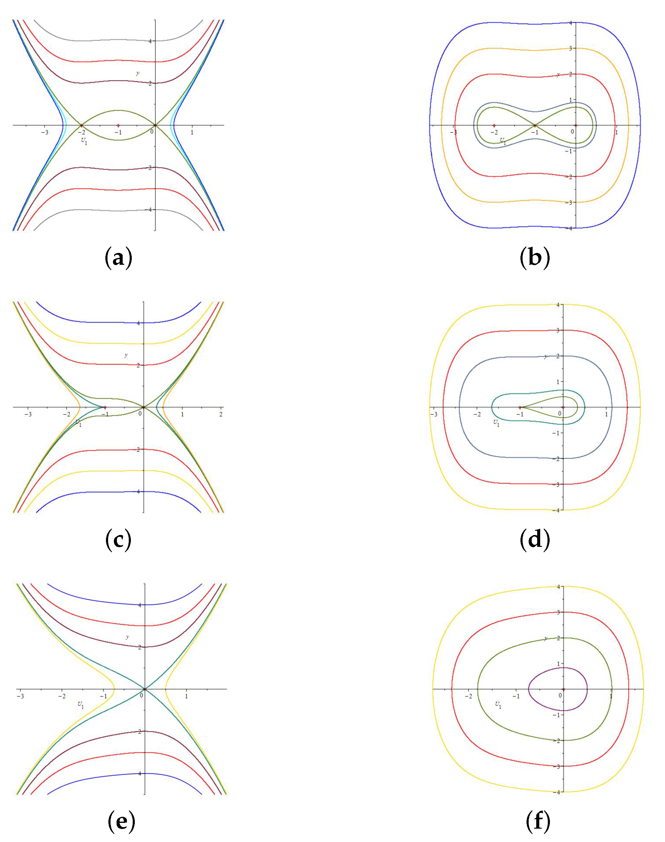
2.2. Phase Portraits of System (9)

Firstly, a two-dimensional dynamics system of Equation (9) can be written as:

$$\left\{\begin{array}{c}\frac{d{U}_j}{d\xi }=y,\hfill \\ \frac{dy}{d\xi }=A_j{U}_j^3+B_j{U}_j^2+C_j{U}_j,\hfill \end{array}\right.$$

(10)

then, the Hamiltonian function of system (10) is defined by

$$H(U_j,y)=\frac{1}{2}{y}_j^2-\frac{A_j}{4}{U}_j^4-\frac{B_j}{3}{U}_j^3-\frac{C_j}{2}{U}_j^2=h,j=1,2,$$

(11)

where h is the constant of integration.

Let $\mathbf{E}(U_j,0)$ be the coefficient matrices of (11) at the equilibrium point $U_j$. The Jacobi determinant of system (10) is defined as $\mathbf{J}\left(U_j\right)=\mathbf{det}\left(\mathbf{E}(U_j,0)\right)=-f^{\prime }\left(U_j\right)$, where $U_j$ is the root of the function $f\left(U_j\right)=A_j{U}_j^3+B_j{U}_j^2+C_j{U}_j$. Then, the phase portraits of system (11) can be drawn as shown in Figure 1.

In Figure 1a, $\mathbf{E}(-2,0)$ and $\mathbf{E}(0,0)$ stand for saddle points, $\mathbf{E}(-1,0)$ represents the center point when $a_1=1, a_2=\frac{7}{8}, b_1=2, b_2=2, c_1=3, d_1=1, \sigma =\frac{1}{2}, k=1$ and $w=\frac{3}{4}$. In Figure 1b, $\mathbf{E}(-2,0)$ and $\mathbf{E}(-1,0)$ represent center points. $\mathbf{E}(-1,0)$ stands for the saddle point when $a_1=1, a_2=1, b_1=2, b_2=\frac{4}{3}, c_1=-3, d_1=-1, \sigma =\frac{1}{2}, k=1$ and $w=-\frac{3}{4}$. In Figure 1c, $\mathbf{O}(0,0)$ represents a center point when $a_1=1, a_2=\frac{1}{2}, b_1=2, b_2=\frac{4}{3}, c_1=2, d_1=1, \sigma =\frac{1}{2}, k=1$ and $w=\frac{9}{4}$. In Figure 1d, $\mathbf{O}(0,0)$ represents a center point when $a_1=1, a_2=\frac{1}{2}, b_1=2, b_2=1, c_1=-2, d_1=-1, \sigma =\frac{1}{4}, k=1$ and $w=\frac{1}{4}$. In Figure 1e, $\mathbf{O}(0,0)$ stands for a center point when $a_1=1, a_2=\frac{1}{2}, b_1=2, b_2=\frac{1}{4}, c_1=2, d_1=1, \sigma =\frac{1}{4}, k=1$ and $w=\frac{13}{4}$. In Figure 1f, $\mathbf{O}(0,0)$ represents a center point when $a_1=1, a_2=\frac{1}{2}, b_1=b_2=2, c_1=-2, d_1=-1, \sigma =\frac{1}{4}, k=1$ and $w=-\frac{3}{4}$.

Remark 1.

The method of studying traveling wave solutions of nonlinear partial differential equations by using the bifurcation theory of plane dynamic systems was first proposed by Professor Li Jibin. In this method, a Hamiltonian system is obtained by using a two-dimensional planar dynamic system, and the phase portraits of the two-dimensional planar dynamic system are drawn.

2.3. Chaotic Behaviors of (2)

Substituting (3) into Equation (2), we can obtain the real parts as

$$\left\{\begin{array}{c}(a_1-b_{1}c)U_1^{{}^{″}}+[(b_{1}k-1)(w-{\sigma }^2)-a_1{k}^2]U_1+c_1{U}_1{U}_2+d_1{U}_1^3=g_1\left(\xi \right),\hfill \\ (a_2-b_{2}c)U_2^{{}^{″}}+[2(2b_{2}k-1)(w-{\sigma }^2)-4a_2{k}^2+c_2)U_2+d_2{U}_1^2+\delta U_1^2{U}_2=g_2\left(\xi \right),\hfill \end{array}\right.$$

(12)

where the imaginary part of Equation (5) remains unchanged.

Let $g_1\left(\xi \right)=(a_1-b_{1}c)f_{0}cos\left(\kappa \xi \right)$ and $g_2\left(\xi \right)=(a_2-b_{2}c)f_{0}cos\left(\kappa \xi \right)$. Then, a two-dimensional disturbance system with a perturbation term is considered as below:

$$\left\{\begin{array}{c}\frac{d{U}_j}{d\xi }=y,\hfill \\ \frac{dy}{d\xi }=A_j{U}_j^3+B_j{U}_j^2+C_j{U}_j+f_{0}cos\left(\kappa \xi \right),\hfill \end{array}\right.$$

(13)

where $f_0$ is the amplitude of (13). $\kappa$ is the frequency of (13).

In Figure 2, Figure 3, Figure 4 and Figure 5, a two-dimensional phase portrait, a three-dimensional phase portrait and the sensitivity of system (13) are presented to give different initial values and parameters, respectively. Obviously, in Figure 2, when the initial value of system (13) changes, the two-dimensional phase diagram of system (13) shows chaotic behavior compared to Figure 1b. Moreover, as shown in Figure 3 and Figure 4, when the initial value changes, the three-dimensional phase diagram and the sensitivity of system (13) further verify the existence of chaotic behavior.

3. Embedded Solitons of System (1)

Multiplying both sides of Equation (9) by $U_j^{\prime }$ and integrating again yields

$${\left(U_j^{\prime }\right)}^2=\frac{A_j}{2}{U}_j^4+\frac{2B_j}{3}{U}_j^3+C_j{U}_j^2+2D_j,$$

(14)

where $D_j$($j=1,2$) is the integral constant.

3.1. $D_j=0$

Let $\Delta =\frac{4}{9}{B}_j^2-2A_j{C}_j$, where $\Delta$ is the discriminant of the polynomial $\Psi \left(U_j\right)=\frac{A_j}{2}{U}_j^2+\frac{2B_j}{3}{U}_j+C_j$. Then, we have

$$\int \frac{d{U}_j}{U_j\sqrt{\frac{A_j}{2}{U}_j^2+\frac{2B_j}{3}{U}_j+C_j}}=\pm (\xi -{\xi }_0).$$

(15)

According to the second-order polynomial complete discrimination system method, the solution of Equation (15) can have the following three forms.

Case 1.1 $\Delta =0$

From Formula (15), it can be obtained that

$$\pm \frac{2B_j}{3A_j}\sqrt{|\frac{A_j}{2}|}(\xi -{\xi }_0)=\mathbf{In}|\frac{U_j-\frac{2B_j}{3A_j}}{U_j}|.$$

(16)

Case 1.2 $\Delta >0$

When $A_j>0$, it can be obtained from Formula (15) that

$$\pm \sqrt{\frac{A_j}{2}}(\xi -{\xi }_0)=\frac{1}{\sqrt{\beta \gamma }}\mathbf{In}\frac{{[\sqrt{(-\gamma )(U_j-\beta )}-\sqrt{(-\beta )(U_j-\beta )}]}^2}{|U_j|},$$

(17)

$$\pm \sqrt{\frac{A_j}{2}}(\xi -{\xi }_0)=\frac{1}{\sqrt{\beta \gamma }}\mathbf{In}\frac{{[\sqrt{\gamma (U_j-\beta )}-\sqrt{\beta (U_j-\beta )}]}^2}{|U_j|},$$

(18)

$$\pm \sqrt{\frac{A_j}{2}}(\xi -{\xi }_0)=\frac{1}{\sqrt{-\beta \gamma }}arcsin\frac{{[\sqrt{(-\gamma )(U_j-\beta )}+\sqrt{(-\beta )(U_j-\beta )}]}^2}{|U_j\left|\right|\beta -\gamma |},$$

(19)

and when $A_j<0$, it can be obtained from Formula (15) that

$$\pm \sqrt{-\frac{A_j}{2}}(\xi -{\xi }_0)=\frac{1}{\sqrt{-\beta \gamma }}\mathbf{In}\frac{{[\sqrt{(-\gamma )(U_j+\beta )}-\sqrt{\beta (U_j-\beta )}]}^2}{|U_j|},$$

(20)

$$\pm \sqrt{-\frac{A_j}{2}}(\xi -{\xi }_0)=\frac{1}{\sqrt{-\beta \gamma }}\mathbf{In}\frac{{[\sqrt{\gamma (-U_j+\beta )}-\sqrt{(-\beta )(U_j-\beta )}]}^2}{|U_j|},$$

(21)

$$\pm \sqrt{-\frac{A_j}{2}}(\xi -{\xi }_0)=\frac{1}{\sqrt{\beta \gamma }}arcsin\frac{{[\sqrt{(-\gamma )(U_j+\beta )}-\sqrt{\beta (U_j-\beta )}]}^2}{|U_j|},$$

(22)

where $\beta =-\frac{2B_j-3\sqrt{\Delta }}{3A_j}$ and $\gamma =-\frac{2B_j+-3\sqrt{\Delta }}{3A_j}$.

Case 1.3 $\Delta <0$

From Formula (15), it can be obtained that

$$\pm \sqrt{\frac{A_j}{2}}(\xi -{\xi }_0)=\sqrt{C_j}\mathbf{In}|\frac{-\frac{3}{4B_j\sqrt{C_j}}{U}_j+\sqrt{C_j}-\sqrt{\frac{A_j}{2}{U}_j^2-\frac{2B_j}{3}{U}_j+C_j}}{U_j}|,$$

(23)

where $C_j>0$.

3.2. $B_j=0$

Let $U_j=\pm \sqrt{{\left(2A_j\right)}^{-\frac{1}{3}}{V}_j}$, ${\rho }_{1j}=4C_j{\left(2A_j\right)}^{-\frac{2}{3}}$, ${\rho }_{0j}=8D_j{\left(2A_j\right)}^{-\frac{2}{3}}$ and ${\xi }_1={\left(2A_j\right)}^{\frac{1}{3}}\xi$. Then, Equation (14) can be written as

$${(\frac{d{V}_j}{d{\xi }_1})}^2=V_j(V_j^2+{\rho }_{1j}{V}_j+{\rho }_{0j}).$$

(24)

Here, we use $\Delta ={\rho }_{1j}^2-4{\rho }_{0j}$ to express the discriminant of the polynomial $\Phi \left(V_j\right)=V_j^2+{\rho }_{1j}{V}_j+{\rho }_{0j}$. Thus, the integral expression of Equation (24) can be expressed as below

$$\pm ({\xi }_1-{\xi }_0)=\int \frac{d{V}_j}{\sqrt{V_j(V_j^2+{\rho }_{1j}{V}_j+{\rho }_{0j})}}.$$

(25)

Case 2.1 $\Delta =0$, $V_j>0$.

When ${\rho }_{1j}<0$, $A_j>0$ and $C_j<0$, the embedded solitons of Equation (1) can be given as

$$u_1(t,x)=\pm {(-\frac{C_1}{A_1})}^{\frac{1}{2}}|tanh(\frac{1}{2}{(-2C_1)}^{\frac{1}{2}}(x-ct-{\xi }_0))|{\mathbf{e}}^{\mathbf{i}(-kx+wt+\sigma W(t)-{\sigma }^{2}t)}.$$

(26)

$$v_1(t,x)=\pm {(-\frac{C_2}{A_2})}^{\frac{1}{2}}|tanh(\frac{1}{2}{(-2C_2)}^{\frac{1}{2}}(x-ct-{\xi }_0))|{\mathbf{e}}^{\mathbf{2}\mathbf{i}(-kx+wt+\sigma W(t)-{\sigma }^{2}t)}.$$

(27)

$$u_2(t,x)=\pm {(-\frac{C_1}{A_1})}^{\frac{1}{2}}|coth(\frac{1}{2}{(-2C_1)}^{\frac{1}{2}}(x-ct-{\xi }_0))|{\mathbf{e}}^{\mathbf{i}(-kx+wt+\sigma W(t)-{\sigma }^{2}t)}.$$

(28)

$$v_2(t,x)=\pm {(-\frac{C_2}{A_2})}^{\frac{1}{2}}|coth(\frac{1}{2}{(-2C_2)}^{\frac{1}{2}}(x-ct-{\xi }_0))|{\mathbf{e}}^{\mathbf{2}\mathbf{i}(-kx+wt+\sigma W(t)-{\sigma }^{2}t)}.$$

(29)

Here, the diagrams of the solution $u_1(t,x)$ of Equation (1) are shown in Figure 6.

When ${\rho }_{1j}>0$, $A_j>0$ and $C_j>0$, the embedded solitons of Equation (1) can be given as

$$u_3(t,x)=\pm {(\frac{C_1}{A_1})}^{\frac{1}{2}}|tan(\frac{1}{2}{(2C_1)}^{\frac{1}{2}}(x-ct-{\xi }_0))|{\mathbf{e}}^{\mathbf{i}(-kx+wt+\sigma W(t)-{\sigma }^{2}t)}.$$

(30)

$$v_3(t,x)=\pm {(\frac{C_2}{A_2})}^{\frac{1}{2}}|tan(\frac{1}{2}{(2C_2)}^{\frac{1}{2}}(x-ct-{\xi }_0))|{\mathbf{e}}^{\mathbf{2}\mathbf{i}(-kx+wt+\sigma W(t)-{\sigma }^{2}t)}.$$

(31)

When ${\rho }_{1j}=0$, $A_j>0$ and $C_j=0$, the embedded solitons of Equation (1) can be given as

$$u_4(t,x)=\pm \frac{2}{|{(2A_1)}^{\frac{1}{2}}(x-ct)-{\xi }_0|}{\mathbf{e}}^{\mathbf{i}(-kx+wt+\sigma W(t)-{\sigma }^{2}t)}.$$

(32)

$$v_4(t,x)=\pm \frac{2}{|{(2A_2)}^{\frac{1}{2}}(x-ct)-{\xi }_0|}{\mathbf{e}}^{\mathbf{2}\mathbf{i}(-kx+wt+\sigma W(t)-{\sigma }^{2}t)}.$$

(33)

Here, the diagrams of the solution $u_3(t,x)$ of Equation (1) are shown in Figure 7.

Case 2.2 $\Delta >0$, $D_j=0$, $V_j>{\rho }_{1j}$

When ${\rho }_{1j}<0$, $A_j>0$ and $C_j>0$, the embedded solitons of Equation (1) can be given as

$$u_5(t,x)=\pm {[-\frac{2C_1}{A_1}+\frac{C_1}{A_1}{tanh}^2(\frac{1}{2}{(2C_1)}^{\frac{1}{2}}(x-ct-{\xi }_0))]}^{\frac{1}{2}}{\mathbf{e}}^{\mathbf{i}(-kx+wt+\sigma W(t)-{\sigma }^{2}t)}.$$

(34)

$$v_5(t,x)=\pm {[-\frac{2C_2}{A_2}+\frac{C_2}{A_2}{tanh}^2(\frac{1}{2}{(2C_2)}^{\frac{1}{2}}(x-ct-{\xi }_0))]}^{\frac{1}{2}}{\mathbf{e}}^{\mathbf{2}\mathbf{i}(-kx+wt+\sigma W(t)-{\sigma }^{2}t)}.$$

(35)

$$u_6(t,x)=\pm {[-\frac{2C_1}{A_1}+\frac{C_1}{A_1}{coth}^2(\frac{1}{2}{(2C_1)}^{\frac{1}{2}}(x-ct-{\xi }_0))]}^{\frac{1}{2}}{\mathbf{e}}^{\mathbf{i}(-kx+wt+\sigma W(t)-{\sigma }^{2}t)}.$$

(36)

$$v_6(t,x)=\pm {[-\frac{2C_2}{A_2}+\frac{C_2}{A_2}{coth}^2(\frac{1}{2}{(2C_2)}^{\frac{1}{2}}(x-ct-{\xi }_0))]}^{\frac{1}{2}}{\mathbf{e}}^{\mathbf{2}\mathbf{i}(-kx+wt+\sigma W(t)-{\sigma }^{2}t)}.$$

(37)

When ${\rho }_{1j}<0$, $A_j>0$ and $C_j<0$, the embedded solitons of Equation (1) can be given as

$$u_7(t,x)=\pm {[-\frac{2C_1}{A_1}-\frac{C_1}{A_1}{tan}^2(\frac{1}{2}{(-2C_1)}^{\frac{1}{2}}(x-ct-{\xi }_0))]}^{\frac{1}{2}}{\mathbf{e}}^{\mathbf{i}(-kx+wt+\sigma W(t)-{\sigma }^{2}t)}.$$

(38)

$$v_7(t,x)=\pm {[-\frac{2C_2}{A_2}-\frac{C_2}{A_2}{tan}^2(\frac{1}{2}{(-2C_2)}^{\frac{1}{2}}(x-ct-{\xi }_0))]}^{\frac{1}{2}}{\mathbf{e}}^{\mathbf{2}\mathbf{i}(-kx+wt+\sigma W(t)-{\sigma }^{2}t)}.$$

(39)

Case 2.3 $\Delta >0$, $D_j\ne 0$, $A_j>0$

Suppose that there are three numbers $\alpha$, $\beta$ and $\gamma$ satisfying $\alpha <\beta <\gamma$. One of them is zero, and the other two are the roots of $\Phi (V_j)$. Then, when $\alpha <V_j<\beta$, the embedded solitons of Equation (1) are given by

$$\begin{array}{cc}\hfill u_8(t,x)& =\pm {(2A_1)}^{-\frac{1}{6}}{[\alpha +(\beta -\alpha ){\mathbf{sn}}^2(\frac{{(\gamma -\alpha )}^{\frac{1}{2}}}{2}{(2A_1)}^{\frac{1}{3}}(x-ct-{\xi }_0),m)]}^{\frac{1}{2}}\hfill \\ \hfill & {\mathbf{e}}^{\mathbf{i}(-kx+wt+\sigma W(t)-{\sigma }^{2}t)}.\hfill \end{array}$$

(40)

$$\begin{array}{cc}\hfill v_8(t,x)& =\pm {(2A_2)}^{-\frac{1}{6}}{[\alpha +(\beta -\alpha ){\mathbf{sn}}^2(\frac{{(\gamma -\alpha )}^{\frac{1}{2}}}{2}{(2A_2)}^{\frac{1}{3}}(x-ct-{\xi }_0),m)]}^{\frac{1}{2}}\hfill \\ \hfill & {\mathbf{e}}^{\mathbf{2}\mathbf{i}(-kx+wt+\sigma W(t)-{\sigma }^{2}t)}.\hfill \end{array}$$

(41)

When $V_j>\gamma$, the embedded solitons of Equation (1) are given by

$$u_9(t,x)=\pm {(2A_1)}^{-\frac{1}{6}}{[\frac{-\beta {\mathbf{sn}}^2(\frac{{(\gamma -\alpha )}^{\frac{1}{2}}{(A_1)}^{\frac{1}{3}}(x-ct-{\xi }_0)}{2},m)+\gamma }{{\mathbf{cn}}^2(\frac{{(\gamma -\alpha )}^{\frac{1}{2}}{(A_1)}^{\frac{1}{3}}(x-ct-{\xi }_0)}{2},m)}]}^{\frac{1}{2}}{\mathbf{e}}^{\mathbf{i}(-kx+wt+\sigma W(t)-{\sigma }^{2}t)},$$

(42)

$$v_9(t,x)=\pm {(2A_2)}^{-\frac{1}{6}}{[\frac{-\beta {\mathbf{sn}}^2(\frac{{(\gamma -\alpha )}^{\frac{1}{2}}{(A_2)}^{\frac{1}{3}}(x-ct-{\xi }_0)}{2},m)+\gamma }{{\mathbf{cn}}^2(\frac{{(\gamma -\alpha )}^{\frac{1}{2}}{(A_2)}^{\frac{1}{3}}(x-ct-{\xi }_0)}{2},m)}]}^{\frac{1}{2}}{\mathbf{e}}^{\mathbf{2}\mathbf{i}(-kx+wt+\sigma W(t)-{\sigma }^{2}t)},$$

(43)

where $m^2=\frac{\beta -\alpha }{\gamma -\alpha }$.

Case 2.4 $\Delta <0$, $A_j>0$

When $V_j>0$, the embedded solitons of Equation (1) are given by

$$\begin{array}{cc}\hfill u_{10}(t,x)& =\pm {(2A_1)}^{-\frac{1}{6}}{[\frac{4{(2D_1)}^{\frac{1}{2}}{(2A_1)}^{-\frac{1}{3}}}{1+\mathbf{cn}({(8D_1)}^{\frac{1}{4}}{(2A_1)}^{-\frac{1}{6}}(x-ct-{\xi }_0),m)}-{(8D_1)}^{\frac{1}{2}}{(2A_1)}^{-\frac{1}{3}}]}^{\frac{1}{2}}\hfill \\ \hfill & {\mathbf{e}}^{\mathbf{i}(-kx+wt+\sigma W(t)-{\sigma }^{2}t)},\hfill \end{array}$$

(44)

$$\begin{array}{cc}\hfill v_{10}(t,x)& =\pm {(2A_2)}^{-\frac{1}{6}}{[\frac{4{(2D_2)}^{\frac{1}{2}}{(2A_2)}^{-\frac{1}{3}}}{1+\mathbf{cn}({(8D_2)}^{\frac{1}{4}}{(2A_2)}^{-\frac{1}{6}}(x-ct-{\xi }_0),m)}-{(8D_2)}^{\frac{1}{2}}{(2A_2)}^{-\frac{1}{3}}]}^{\frac{1}{2}}\hfill \\ \hfill & {\mathbf{e}}^{\mathbf{2}\mathbf{i}(-kx+wt+\sigma W(t)-{\sigma }^{2}t)},\hfill \end{array}$$

(45)

where $m^2=\frac{1-\frac{C_j}{{\left(2D_j\right)}^{\frac{1}{2}}{\left(2A_j\right)}^{\frac{1}{3}}}}{2}$.

4. Discuss

Compared with ref. [18], we also obtained the exponential function solutions, Jacobian function solutions and implicit solutions of Equation (1). These are not reported in ref. [18] (see

Table 1. Comparison between our results and ref. [18].

	Results	Our Results	Results of Ref. [18]
Type of Solutions
Exponential function solutions		$u_4(t,x)$, $v_4(t,x)$,
Trigonometric function solutions		$u_7(t,x)$, $v_7(t,x)$,	Solutions (19), (31)∼(34),
			Solutions (50), (51), (58), (59),
Rational function solutions			Solutions (37), (38)
Hyperbolic function solutions		$u_5(t,x)$, $v_5(t,x)$,	Solutions (18), (25)∼(30),
			Solutions (48), (49), (56), (57),
		$u_6(t,x)$, $v_6(t,x)$,
Jacobi elliptic function solutions		$u_8(t,x)\sim u_{10}(t,x)$,
		$v_8(t,x)\sim v_{10}(t,x)$,
Implicit function solutions		Solutions (16)∼(23)

).

5. Conclusions

In this paper, the theory of plane dynamics systems has been utilized to study the dynamic behavior and embedded soliton solutions of (1) and the dynamic behavior, chaotic behavior and sensitivity of (2). Two-dimensional phase portraits of the dynamic system of (1) have been drawn in Maple software. Moreover, two-dimensional and three-dimensional phase portraits and the sensitivity of (2) have been plotted. From the literature [18], it can be seen that not only were the embedded solitons of (1) obtained by using the complete discrimination system method, but the chaotic behavior and sensitivity of (2) was also further analyzed. In the future, the dynamics and soliton solutions of more complex SPDEs will be studied.

References

1. Fujioka, J.; Espinosa-Cerón, A.; Rodriguez, R. A survey of embedded solitons. Rev. Mex. Fis. 2006, 52, 6–14. [Google Scholar]
2. Yang, J.; Malomed, B.A.; Kaup, D.J.; Champneys, A.R. Embedded solitons: A new type of solitary wave. Math. Comput. Simul. 2001, 56, 585–600. [Google Scholar] [CrossRef] [Green Version]
3. Tan, Y.; Yang, J.K.; Pelinovsky, D.E. Semi-stability of embedded solitons in the general fifth-order KdV equation. Wave Motion 2002, 36, 241–255. [Google Scholar] [CrossRef] [Green Version]
4. Sonmezoglu, A.; Ekici, M.; Arnous, A.H.; Zhou, Q.; Triki, H.; Moshokoa, S.P.; Ullah, M.Z.; Biswas, A.; Belic, M. Embedded solitons with χ(2) and χ(3) nonlinear susceptibilities by extended trial equation method. Optik 2018, 154, 1–9. [Google Scholar] [CrossRef]
5. Susanto, H.; Malomed, B.A. Embedded solitons in second-harmonic-generating lattices. Chaos Solitons Fractals 2021, 142, 110534. [Google Scholar] [CrossRef]
6. Kudryashov, N.A. Exact solutions of equation for description of embedded solitons. Optik 2022, 268, 169801. [Google Scholar] [CrossRef]
7. Smith, T.B.; Choudhury, S.R. Regular and embedded solitons in a generalized pochammer PDE. Commun. Nonlinear Sci. Numer. Simul. 2009, 14, 2637–2641. [Google Scholar] [CrossRef]
8. Animasaun, I.I.; Shah, N.A.; Wakif, A.; Mahanthesh, B.; Sivaraj, R.; Koriko, O.K. Ratio of Momentum Diffusivity to Thermal Diffusivity; Chapman and Hall/CRC: New York, NY, USA, 2022. [Google Scholar]
9. Zayed, E.M.E.; Alngar, M.E.M.; Shohib Reham, M.A. Cubic-quartic embedded solitons with χ(2) and χ(3) nonlinear susceptibilities having multiplicative white noise via Itô Calculus. Chaos Solitons Fractals 2023, 168, 113186. [Google Scholar] [CrossRef]
10. Chen, Z.M.; Zeng, J.H. Two-dimensional optical gap solitons and vortices in a coherent atomic ensemble loaded on optical lattices. Commun. Nonlinear Sci. Numer. Simul. 2021, 102, 105911. [Google Scholar] [CrossRef]
11. Palmero, F.; Molina, M.I.; Guevas-Maraver, J.; Kevrekidis, P.G. Discrete embedded solitary waves and breathers in one-dimensional nonlinear lattices. Phys. Lett. A 2022, 425, 127880. [Google Scholar] [CrossRef]
12. Han, T.Y.; Li, Z.; Zhang, K. Exact solutions of the stochastic fractional long-short wave interaction system with multiplicative noise in generalized elastic medium. Results Phys. 2023, 44, 106174. [Google Scholar] [CrossRef]
13. Zayed, E.M.E.; Shohib, R.M.A.; Alngar, M.E.M. Dispersive optical solitons in magneto-optic waveguides with stochastic generalized Schrödinger-Hirota equation having multiplicative white noise. Optik 2022, 271, 170069. [Google Scholar] [CrossRef]
14. He, T.; Wang, Y.Y. Dark-multi-soliton and soliton molecule solutions of stochastic nonlinear Schrödinger equation in the white noise space. Appl. Math. Lett. 2021, 121, 107405. [Google Scholar] [CrossRef]
15. Li, W.; Tian, B. Stochastic solitons in a two-layer fluid system. Chin. J. Phys. 2023, 81, 155–161. [Google Scholar] [CrossRef]
16. Li, Z.; Huang, C.; Wang, B.J. Phase portrait, bifurcation, chaotic pattern and optical soliton solutions of the Fokas-Lenells equation with cubic-quartic dispersion in optical fibers. Phys. Lett. A 2023, 465, 128714. [Google Scholar] [CrossRef]
17. Li, Z.; Huang, C. Bifurcation, phase portrait, chaotic pattern and optical soliton solutions of the conformable Fokas-Lenells model in optical fibers. Chaos Solitons Fractals 2023, 169, 113237. [Google Scholar] [CrossRef]
18. Zayed, E.M.E.; Alngar, M.E.M.; Shohib, R.M.A.; Biswas, A.; Yıldırım, Y.; Moraru, L.; Mereuta, E.; Alshehri, H.M. Embedded solitons with χ(2) and χ(3) nonlinear susceptibilities having multiplicative white noise in the Itô Calculus. Chaos Solitons Fractals 2022, 162, 112494. [Google Scholar] [CrossRef]
19. Rao, R.; Lin, Z.; Ai, X.; Wu, J. Synchronization of epidemic systems with Neumann boundary value under delayed impulse. Mathematics 2022, 10, 2064. [Google Scholar] [CrossRef]
20. Li, G.D.; Zhang, Y.; Guan, Y.J.; Li, W.J. Stability analysis of multi-point boundary conditions for fractional differential equation with non-instantaneous integral impulse. Math. Biosci. Eng. 2023, 20, 7020–7041. [Google Scholar] [CrossRef]
21. Zhao, Y.; Wang, L. Practical exponential stability of impulsive stochastic food chain system with time-varying delays. Mathematics 2023, 11, 147. [Google Scholar] [CrossRef]
22. Li, K.; Li, R.; Cao, L.; Feng, Y.; Onasanya, B.O. Periodically intermittent control of Memristor-based hyper-chaotic bao-like system. Mathematics 2023, 11, 1264. [Google Scholar] [CrossRef]
23. Xia, M.; Liu, L.; Fang, J.; Zhang, Y. Stability analysis for a class of stochastic differential equations with impulses. Mathematics 2023, 11, 1541. [Google Scholar] [CrossRef]
24. Xue, Y.; Han, J.; Tu, Z.; Chen, X. Stability analysis and design of cooperative control for linear delta operator system. AIMS Math. 2023, 8, 12671–12693. [Google Scholar] [CrossRef]
25. Tang, Y.; Zhou, L.; Tang, J.; Rao, Y.; Fan, H.; Zhu, J. Hybrid impulsive pinning control for mean square synchronization of uncertain multi-link complex networks with stochastic characteristics and hybrid delays. Mathematics 2023, 11, 1697. [Google Scholar] [CrossRef]
26. Wang, C.; Liu, X.; Jiao, F.; Mai, H.; Chen, H.; Lin, R. Generalized Halanay inequalities and relative application to time-delay dynamical systems. Mathematics 2023, 11, 1940. [Google Scholar] [CrossRef]
27. Ma, Z.; Yuan, S.; Meng, K.; Mei, S. Mean-square stability of uncertain delayed stochastic systems driven by G-Brownian motion. Mathematics 2023, 11, 2405. [Google Scholar] [CrossRef]
28. Wang, C.; Song, Y.; Zhang, F.; Zhao, Y. Exponential stability of a class of neutral inertial neural networks with multi-proportional delays and leakage delays. Mathematics 2023, 11, 2596. [Google Scholar] [CrossRef]
29. Yang, Q.; Wang, X.; Cheng, X.; Du, B.; Zhao, Y. Positive periodic solution for neutral-type integral differential equation arising in epidemic model. Mathematics 2023, 11, 2701. [Google Scholar] [CrossRef]
30. Li, J.B.; Dai, H.H. On the Study of Singular Nonlinear Traveling Wave Solutions: Dynamical System Approach; Science Press: Beijing, China, 2007. [Google Scholar]
Figure 1. Two-dimensional phase portraits of (10) for j = 1 . (a) A 1 > 0 ,   B 1 > 0 ,   C 1 > 0 ,   B 1 2 > 4 A 1 C 1 . (b) A 1 < 0 ,   B 1 < 0 ,   C 1 < 0 ,   B 1 2 > 4 A 1 C 1 . (c) A 1 > 0 ,   B 1 > 0 ,   C 1 > 0 ,   B 1 2 = 4 A 1 C 1 . (d) A 1 < 0 ,   B 1 < 0 ,   C 1 < 0 ,   B 1 2 = 4 A 1 C 1 . (e) A 1 > 0 ,   B 1 > 0 ,   C 1 > 0 ,   B 1 2 < 4 A 1 C 1 . (f) A 1 < 0 ,   B 1 < 0 ,   C 1 < 0 ,   B 1 2 < 4 A 1 C 1 .
Mathematics 11 03185 g001
Figure 2. Two-dimensional phase portrait of system (13) for a 1 = 1 ,   a 2 = 1 ,   b 1 = 2 ,   b 2 = 4 3 ,   c 1 = 3 ,   d 1 = 1 ,   σ = 1 2 ,   k = 1 , w = 3 4 and j = 1 .
Mathematics 11 03185 g002
Figure 3. Three-dimensional phase portrait of system (13) for a 1 = 1 ,   a 2 = 1 ,   b 1 = 2 ,   b 2 = 4 3 ,   c 1 = 3 ,   d 1 = 1 ,   σ = 1 2 ,   k = 1 , w = 3 4 and j = 1 .
Mathematics 11 03185 g003
Figure 4. Sensitivity of system (13) for a 1 = 1 ,   a 2 = 1 ,   b 1 = 2 ,   b 2 = 4 3 ,   c 1 = 3 ,   d 1 = 1 ,   σ = 1 2 ,   k = 1 , w = 3 4 and j = 1 .
Mathematics 11 03185 g004
Figure 5. Phase portrait of system (13) for a 1 = 1 ,   a 2 = 1 2 ,   b 1 = b 2 = 2 ,   c 1 = 2 ,   d 1 = 1 ,   σ = 1 4 ,   k = 1 , w = 3 4 and j = 1 .
Mathematics 11 03185 g005
Figure 6. Embedded solitons R e l ( u 1 ( t , x ) ) of system (1) for a 1 = 1 ,   b 1 = 2 ,   b 2 = 2 ,   c 1 = 0 ,   c = 1 ,   d 1 = 1 2 ,   σ = 2 , k = 1 and w = 4 .
Mathematics 11 03185 g006
Figure 7. Embedded solitons R e l ( u 3 ( t , x ) ) of system (1) for a 1 = 1 ,   b 1 = 2 ,   c 1 = 0 ,   c = 1 ,   d 1 = 1 2 ,   σ = 1 ,   k = 1 and w = 3 .
Mathematics 11 03185 g007