Article

Control Factors for the Equilibrium Composition of Microbial Communities in Open Systems: Theory and Experiments

by
Andrey Degermendzhi
1 and
Alexander Abakumov
2,*
1
Institute of Biophysics, Department of Federal Research Center “Krasnoyarsk Science Center of the Siberian Branch of the Russian Academy of Sciences”, 660036 Krasnoyarsk, Russia
2
Institute for Automation and Control Processes, Far Eastern Branch, Russian Academy of Sciences, 690041 Vladivostok, Russia
*
Author to whom correspondence should be addressed.
Mathematics 2023, 11(14), 3183; https://doi.org/10.3390/math11143183
Submission received: 23 June 2023 / Revised: 17 July 2023 / Accepted: 18 July 2023 / Published: 20 July 2023
(This article belongs to the Special Issue Mathematical Modeling of Evolutionary Dynamics)

Abstract

:
The present paper is a summary of the authors’ theoretical and experimental research dealing with the patterns of stable equilibrium coexistence of microbial populations in flow systems interacting through specific density-dependent growth regulators (RFs). The discovered “paradoxical” lack of dependence of the background steady-state levels (concentrations) of RFs on their input values is confirmed experimentally and theoretically through the introduced sensitivity coefficients. This effect has been termed “autostabilization” of RFs. An important theorem (formula) of “quantization” suggesting the integer value of the sum of all sensitivity coefficients, which is equal to the difference between the number of RFs and the number of populations of one trophic level, has been proven. A modification of the “quantization” formula for an arbitrary trophic web is shown. A new criterion for intra- and inter-population microbial interactions for RFs is proposed—the response of growth acceleration to a perturbation in population size. This criterion makes it possible to quantify interspecific complex relationships, which has been previously impossible. The relationship between the new coefficients of inter-population interactions and the accuracy of model verification has been shown theoretically. Based on this criterion and the autostabilization effect, a method for experimental search for unknown RFs is proposed.

1. Introduction

Modern ecology faces a number of challenges, one of which is controlling the species composition of natural communities. In addition to the fundamental aspect, this is important for such practical tasks as the reestablishment of ecological structures after anthropogenic interventions, including ensuring the proper level of self-purification and finding ways to eliminate “harmful” populations. An open system for continuous cultivation in which steady state is achieved due to the growth rate (cell division) being equal to the flow rate (removal as a mortality analog) will serve as the experimental basis for the theoretical analysis of these problems [1]. An important long-range objective is to use continuous cultures of, e.g., microalgal communities with controlled composition, in closed human life support systems to supply humans with oxygen and to remove CO2 and urine [2]. The key issue of matching the respiratory quotient of the mixed microalgal culture to the respiratory quotient of humans could be solved by controlling the composition of mixed populations of algae that have different respiratory quotients [3].
The general principle leading to controlling the species composition of a community is based on the ecological mechanisms underlying the coexistence of species through the regulation of population growth and mortality. The theory states that a sufficient condition for the coexistence of two species is the prevalence of intraspecific competition over interspecific competition [4,5]. At the same time, two species competing for a common resource cannot coexist, which is termed “the competitive exclusion principle” [6,7]. The “aquatic” analogue of this principle, the “paradox of the plankton” [8], has caused a surge of theoretical research aimed to find various mechanisms that explain the paradox, i.e., an “exclusion” from the “exclusion principle” [9,10,11,12,13,14,15,16,17,18,19,20]. The modes of coexistence considered in different studies are based on a kind of “separation” of competition in space or time, or both. Armstrong and McGehee [13] proved in a theoretically rigorous manner that there is no restriction on the number of coexisting species limited to four resources (substrates) in the self-oscillation mode. The work [21] showed, using a computer model, that there are quite exotic mechanisms for regulating the abundance of two species, leading to “chaotic” coexistence on a single limiting resource. The mechanisms of coexistence proposed by the theory are possible and may exist in nature, but, unfortunately, most of them have not been tested experimentally [22]. The theory of coexistence in its classical form corresponds to mathematical phenomenological models of the form:
X ˙ = X g X ,   Q ,
where Q is a vector of independent factors. Equations similar to (1) can model predatory or direct interactions between species. The classical studies by R. MacArthur and S. Levin [9], S. Levin [23], and R. MacArthur [24] proved that in the equilibrium culture containing several species, their number should not exceed the number of substrates (resources) limiting their growth rate. Thus, the theory states that in equilibrium, out of two populations limited by the same resource, only one species survives [6]. In the general case, regulation of type (1) is termed “density-dependent growth control factor” (DDGCF). However, most experiments and new theoretical approaches deal with DDGCFs that take into account the specific chemical (biochemical, metabolic) or physical nature of these factors. In order to distinguish this type of factors from the classical DDGCFs, these metabolic regulators will be referred to as “regulating factors” (RFs). Depending on the nature of RFs, they influence the specific growth rate of a particular species, while the dynamics of the RFs is determined by the activity of the population or populations.
This study is a theoretical and experimental analysis of stability and controllability of the equilibrium microbial mixture without trophic interactions in perfectly mixed flow systems with special emphasis on RF dynamics. The specific analysis of RFs has also given rise to the new rule of estimating relationships between species based on species growth acceleration in response to a change in the abundance of this or another species. Eventually, special dynamics of RFs and the “growth acceleration” rule will be of critical importance in the experimental search for such RFs in communities, which are real “levers” for controlling species composition.

2. The Rule of Coexistence of Microbial Populations in Continuous Cultures

The classical approach to classifying the interspecific relationships was based on estimating the “sign” and the “value” of the change in specific growth rate of one species as a consequence of an increase in the abundance of another species [25]. Equation (1) serves as the mathematical basis for this approach. In other words, values B ¯ i l = g i X 1 ,   ,   X n ,   t / X l   or   B i l = s i g n   B ¯ i l determine ultimate relationships between species. The “sign” and the “value” of numbers ( B l i ,   B i l ) determine specific types of relationships: (−1, −1) means competition or antagonism, (+1, 0)—commensalism, (−1, 0)—amensalism, etc.
The theory of analysis of relationships between microbial species (numbering m, as an example) in mixed culture should begin with the general model (2) “immersed” in the open flow system. It is assumed that the specific growth rate (SGR) of each population is affected by certain RFs, the total number of which in the system is n. The change in the level of each RF is caused by the uptake or release of this factor by a definite population or a group of populations whose total number is m. Then, system (2) has the following form:
X ˙ = g R D X ,
R ˙ = D R 0 R + f X , R .
The term f X , R in the right-hand part determines the final balance of regulators in the culture. It is difficult to present the function g as dependent on R in some general form, although specific cases, e.g., those involving Liebig’s law, are known. However, even such a general form shows that in the equilibrium mixture, the number of species is no greater than the total number of RFs (i.e., m n ) [26]. The result of coexistence obtained here is similar to the results obtained by other authors addressing regulation via DDGCFs, but the present rule of coexistence includes not only limitation by substrate, but also a large number of other interspecific relationships. The broader condition of species coexistence obviously leads to an extended interpretation of Gause’s principle [27]: not only the single limiting resource–substrate but also any other RF prevents the two species from living together.
If the list of RFs is extended by including various types of regulation of species abundance in flow systems (maintenance of absorbance, concentrations of phytopigments, acidic ions, etc.), the coexistence rule remains valid: the total number of RFs should also include these types of regulation. The chemical processes in the system do not contradict this rule either.
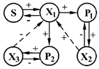
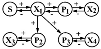
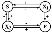
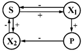
Table 1, reproduced from our previous paper [28], summarizes almost all literature data on experiments with microbial populations coexisting in flow systems, including the specific RFs responsible for that. The table also shows that the coexistence rule holds true: the number of populations is lower than the number of RFs. It is important that the RFs are listed as coexistence mechanisms, and their specific dynamics will be considered below.

Coexistence, Interaction Coefficients, and the New Criterion of Interactions between Populations

The rule of estimating the relationships between microbial species through certain RFs needs to be revised because the growth rate of the “acceptor” population does not immediately respond to the change in the size of the “donor” population: its response is delayed to after the change in the level of the RF. Therefore, the next objective is to rigorously derive this rule of estimating the relationships.
The purpose of this section is to formulate a new interaction criterion “adapted” to models that describe the dynamics of the structure of microbial communities. We use the rather universal description of the coexistence mechanism in the flow system with the RF role explicitly taken into account as the underpinning for our reasoning.
The type of relationship can be determined from changes in one population in response to changes in the size of the other. We assume that the biomass of a species (number l) in the mixture at time t * has increased by the amount Δ X l . Then, the R t * level will not change immediately at time t * , and specific growth rate g R | t * will not change either, as, according to Equation (2), the perturbation Δ X l will only cause a change in the first time derivative R, i.e., a change in R : ˙
R ˙ | t * P l = D R 0 R + f X 1 , , X l + Δ X l , ,   X m ,   R
when compared with the unperturbed value,
R ˙ | t * U = D R 0 R + f X 1 , , X l , X l + 1 , ,   X m ,   R ,
where P is the perturbed state and U is the unperturbed state.
Thus, the time derivative of the specific growth rate, i.e., growth acceleration, will be the parameter of the “acceptor” population” that will “sense” a change in the size of the “donor” population, and, hence, it should be called the new rule of estimating interspecific relationships. A formula that does not require system (2) to be solved was derived for calculating growth acceleration.
Then, the difference between growth accelerations of these two states will be the measure of the type (the plus sign (stimulation) or the minus sign (inhibition)) and magnitude of the interactions between species.
B ¯ i l = g i t t * P l g i t t * U l ,   i = 1 , m ¯ .
Graphically, B ¯ i l is the difference between slope ratios of tangents to the corresponding curves of specific growth rates, which can be determined experimentally. Since g g R , the derivative is given by
g t = g R · R t .
Substituting (3), (4), and (6) into (5) and taking into account the fact that
g / R t * P l = g / R t * U ,
we obtain
B ¯ i l = g i R · R ˙ t * P l g i R · R ˙ t * U = g i R · f t * P l f t * U .
When the perturbation, Δ X l , is sufficiently small, the expression f t * P l f t * U can be replaced by f / X l Δ X l , that is:
B ¯ i l = Δ X l g i R · f X l .
The value of B ¯ i l (7) shows how species number l affects species number i. As a rule, the following option
f = A g R X
is of interest, leading to the interaction coefficients of the form
B ¯ i l = Δ X l g l g i R a l ,
where a l denotes the lth column of matrix A.
Since Δ X l , g l 0 , the type of relationship B i l is determined by the sign of the expression below, simultaneously simplifying the expression by normalizing B ¯ i l per unit of change in the number and unit of specific growth rate:
B i l = s i g n   B ¯ i l = g i R a l .
Coefficients B l i and B i l characterize interactions between two species, and the previously proposed table of interactions [24] can be also used for the new classification. As is easy to see, the type of interaction is constant over time in two cases: if specific growth rate is proportionally related to R and in equilibrium.
Thus, we construct the following matrix of interaction coefficients
B = B i l i , l = 1 m
and obtain the formula
B = g R · A .

3. Sensitivity Coefficients

The presence of the feedback, e.g., in regulation of the growth of monoculture, where the level of the regulator in the culture changes with the change in the growth rate, and, at the same time, the regulator influences specific growth rate, causes “paradoxical” regulator dynamics. The essence of this dynamics is the absence of the relationship(!) between the background level of the regulator and its input flow (at m = n ).
The autostabilization effect can be explained using a simple example of continuous monoculture ( X ) controlled by substrate ( S ). The model has the form
X ˙ = g S D X ,   S ˙ = D S 0 S g S X / Y ,
where g S = g m S / k s + S is specific growth rate of the species; Y is substrate consumption factor; g m is the greatest specific growth rate; k s is coefficient of sensitivity to the growth limiting substrate. The positive steady-state solution of this equation is: X ¯ = Y S 0 S ¯ and S ¯ = k s D / g m D . Hence, substrate concentration ( S ¯ ) does not depend on its input concentration ( S 0 ) in the state of growth limitation. If the autostabilization effect is formalized by introducing the coefficient of autostabilization K = S ¯ / S 0 , then K = 0 , and concentration S ¯ does not depend (!) on input concentration S 0 .
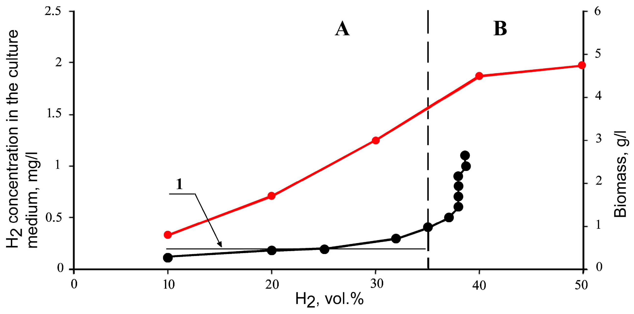
The autostabilization effect can be illustrated with diverse experimental studies, cultivation of hydrogen-oxidizing bacterium Seliberia carboxydohydrogena Z1062 vs. limited by dissolved oxygen being a good example (Figure 1). Figure 2 demonstrates that steady-state concentration of H2 is not related to its input concentration (the ideal line is denoted by 1) in the limitation zone A, while steady-state biomass concentration grows in direct proportion to the input level of the limiting hydrogen. The autostabilization coefficient of the sensitivity coefficient in zone A is approximately equal to zero (slope ratio). The opposite trend is observed on leaving the limitation zone and entering zone B. This example explicitly describes the mechanism of autostabilization of the limiting factor and, generally, any DDGCF type.

3.1. An Invariant for Sensitivity Coefficients

The problem of sensitivity coefficients will be considered for model (2) at f X , R = A g R X :
d X d t = g R D X
d R d t = D R 0 R + A g R X
with n number of RFs and m number of species.
The totality of sensitivity coefficients K 1 ,   ,   K n obeys the law:
K j = R j R j 0 ,
and
j = 1 n K j = n m ,
where R j is RF concentration in steady state. Sensitivity coefficients are the characteristics of RF autostabilization in steady state.
Formula (12) is a rare law of ecology, invariant to the integral property of the species mixture in the open flow system, which are connected by an arbitrarily complex network of biochemical (metabolic) relationships through growth regulators. Its essence is that the sum of all autostabilization coefficients will always be a natural number, and this can be found in special flow experiments. A number of specific properties follow from this law:
(1)
The value of K j for each regulator j, in the general case, will be a fractional number both greater and less than zero, which can change from equilibrium to a new equilibrium when input levels of regulators are varied;
(2)
Although all K j values are variable and non-integer, summation of them always produces the same natural number—deduction of the total number of species in the equilibrium mixture from the total number of regulators;
(3)
It allows us to assess the level of our understanding of the completeness of relationships in a mixture of species: Violation of Formula (12) requires the search for additional regulators and/or new species.
Let us prove the integrity of the sum of sensitivity coefficients. To obtain the result, we need the following data.
Definition 1.
The term trace of square matrix A, tr A, denotes the sum of its diagonal elements [39].
Lemma 1.
For matrices  A = a i j i , j = 1 n , m , B = b i j i , j = 1 m , m , C = c i j i , j = 1 m , n equation, t r A B C = t r C A B is satisfied.
Proof. 
Both matrices in the equation that is being proven are square. The equation is proven by directly calculating the traces of both matrices, leading to the relation.
t r A B C = t r C A B = i , j , k = 1 n , m , m a i j b j k c k i
Next, we proceed to proving the corresponding theorem.
As a preliminary step, we linearize the function of specific growth rate around the equilibrium: g R = G R with matrix G of dimension mxn. □
Theorem 1 of Quantization.
Suppose that matrix G A is non-degenerate. Then, the sum of sensitivity coefficients K = j = 1 n K j in balanced state is equal to n m .
Proof. 
The nontrivial equilibrium solution is determined from equations:
g R D = 0 ,
D R 0 R + A g R X = 0 .
After transformations, we obtain a system of linear algebraic equations:
R A X = R 0 ,
G R = D .
Now we perform a number of transformations. From the Equation (13a), we obtain
R = R 0 + A X .
Having substituted this expression into the Equation (13b)
G A X = G R 0 + D ,
we obtain an expression for X:
X = G A 1 G R 0 + D .
This expression is substituted into Equation (9):
R = I n x n A G A 1   G R 0 + A G A 1 D .
Here, I n x n denotes the identity matrix of the corresponding dimension.
Note that if matrix G A is non-degenerate, the nontrivial equilibrium solution is unique. Its positivity must be assumed additionally.
Because of the linearity of the last relation, sensitivity coefficients K j = R j R j 0 are diagonal elements of matrix I n x n A G A 1   G from Equation (14).
Then
j = 1 n K j = t r   I n x n A G A 1   G   = t r I n x n t r   A G A 1   G = n t r   A G A 1   G .
To calculate the second expression in the last formula, we perform auxiliary transformations. We give the equation:
m = t r I m x m = t r G A 1 G A = t r A G A 1 G .
The last equation is satisfied in accordance with the above lemma.
By substituting the last relation into the previous formula, we obtain
j = 1 n K j = n t r   A G A 1   G = n m .
The theorem has been proven. □
Notes. A necessary condition for the non-degeneracy of the matrix GA is the inequality n ≥ m. This follows from the fact that the rank of non-degenerate matrix must be equal to m. But, the rank of the product of two rectangular matrices does not exceed the rank of each of the factors [42]. The non-degeneracy condition is obviously false for n < m.

3.2. The Generalization Taking into Account the “Non-Factor” Species Interaction

Next, we consider a more general case, in which direct, “non-factor”, species interactions in the community are taken into account. These are mainly the predator–prey interactions. The construction of the previous theorem does not take them into consideration.
Then, Model (10) is generalized as follows:
d X d t = g X , R D X ,
d R d t = D R 0 R + A g X , R X   .
Again, we assume linearization of the function of specific growth rate around the equilibrium:
g X , R = G R + G 0 + H X + H 0
with matrices G , H of coefficients in specific growth rates of dimensions mxn and mxm, respectively; vectors G 0 ,   H 0 have dimension m.
Theorem 2. 
If matrix G A + H is non-degenerate, the sum of sensitivity coefficients K = j = 1 n K j is equal to n m + t r G A + H 1 H .
Proof. 
The nontrivial equilibrium solution is determined from equations:
g X , R D = 0 ,
D R 0 R + A g X , R X   = 0 .
After transformations, we obtain a system of linear algebraic equations:
R A X = R 0
G R + H X = D G 0 + H 0 .
The logic of the proof mainly corresponds to the proof of the previous theorem, but the generalization leads to certain adjustments. From the Equation (16a), we obtain
R = R 0 + A X .
By substituting this expression into the Equation (16b)
G A + H X = G R 0 + D G 0 + H 0 ,
we obtain the expression for X:
X = G A + H 1 G R 0 + D G 0 + H 0 .
Then, we substitute this expression into Equation (17):
R = I n x n A G A + H 1   G R 0 + A G A + H 1 D G 0 + H 0 .
Here I n x n denotes the identity matrix of the corresponding dimension. □
Note that if matrix G A + H is non-degenerate, the nontrivial equilibrium solution is unique. Its positivity must be assumed additionally.
Because of the linearity of the last relation, sensitivity coefficients K j = R j R j 0 are diagonal elements of matrix I n x n A G A + H 1   G from Equation (18).
Then
j = 1 n K j = t r   I n x n A G A + H 1   G   = t r I n x n t r   A G A + H 1   G = n t r   A G A + H 1   G .
To calculate the second expression in Formula (18), we perform auxiliary transformations. We give the equation
m = t r I m x m = t r G A + H 1 G A + H
and transform the last expression:
r G A + H 1 G A + H = t r G A + H 1 G A + G A + H 1 H = t r G A + H 1 G A + t r G A + H 1 H .
We apply the Lemma 1 mentioned above in the first term of the last expression and, as we start these auxiliary transformations, we obtain
m = t r A G A + H 1 G + t r G A + H 1 H .
Hence,
t r A G A + H 1 G = m tr G A + H 1 H .
Having substituted the last expression into Formula (19), we obtain the sought-for formula:
K = j = 1 n K j = n m + t r G A + H 1 H .
The theorem has been proven.
Notes.
(1)
Matrix B (9) of population interactions in the community through factors coincides with G A . Formula (20) can be rewritten as
K = n m + t r B + H 1 H .
(2)
If there are no “non-factor” interactions in the community ( H = 0 ), Theorem 2 gives the result of Theorem 1.
(3)
If the factors do not affect the dynamics of the community ( B = 0 ), the sum of sensitivity coefficients is equal to the number of factors, n, suggesting that the community does not affect the factors either; thus, the community and the factors do not interact. For the community, the factors taken into account are imaginary and fictitious.
(4)
If the effects of “non-factor” interactions and factors in the community are proportional to each other ( H = γ B at some γ 0 ), Formula (21) has the following form: K = n 1 1 + γ m . Then, the condition K n m ,   n is satisfied. One can only assume that the range of K is the same in the general case as well.

3.3. An Invariant for the Theorem of Quantization in the Case of Distribution of Cells by Growth Rate and Age

When proving the “quantization” theorem, we assumed that every species of microorganisms can be characterized by an average biomass growth rate, µ i ( R ) , although, actually, in each population of microorganisms, there is an age distribution: cells of different ages, with the corresponding growth parameters, are present simultaneously. In this regard, one may ask: Will the theorem hold if the specific growth rate of a given species of microorganisms is the function of the biological age of a given cell?
In this problem, we can introduce age and its relationship to specific growth rate in Equation (2). For this, we can add the state variable s, which changes from zero to one during the cell cycle. Then, system (2) is transformed to the form (22a):
X i s , t t + v i R X i s , t s = X i D
d R j d t = R j 0 R j D + k = 1 m 0 1 a j k s v j R X k s , t d s
with the boundary condition
X i 0 , t = 2 X i 1 , t .
Next, we consider another possible case of heterogeneity. For each microorganism, there is some function of distribution by the growth rate, i.e., the same population simultaneously contains “fast” and “slow” cells, which move with different velocities along the phase variable s. For this case, equations describing the growth of cell populations have the following form:
X i v i , s , t t + v i R X i v i , s , t s = X i v i , s , t D ,
d R j d t = R j 0 R j D + k = 1 n v 0 1 a j k s v k R y k v k , s , t d s d v ,
where Xi(s, t) is the abundance of species i at time t in state s; ajk(s) is consumption/release factor of the regulator; vi(R) is the velocity of the ith species of microorganisms moving along the axis of the state. For equilibrium conditions, Equation (22) will have the following form: X i s s = D v i R X i s ,
R j = R j 0 + k = 1 n 0 1 a j k s v k R D X k s d s ,
or, taking into account expression (23), after transformations:
2 = e x p D v i R ,
R j = R j 0 + 1 ln 2 k = 1 m a ˜ j k X k 0 ,
where
a ˜ j k = 0 1 a j k s X k s d s .
The system of Equation (22), with an accuracy to notations, is equivalent to the system of Equation (2). Hence, expression (15) is also valid in this, more complex, model, which takes into consideration cell age dependence of substance transformation. Therefore, in the equilibrium, Equation (24) can be changed to the form analogous to system (2), thus proving the validity of the “quantization” theorem.

4. Experiments with Monocultures

In the general case, the growth of a single species can be controlled by several diverse regulators (RFs) [43,44,45,46]. The question naturally arises as to the choice of the criterion for determining all regulators for the species. The total regulation can be measured using the value of B i l , when i = l. Then, B B i i will be termed feedback coefficient. The theoretical value of feedback B t can be calculated using Formula (9) if the particular regulators and their effect on specific growth rate are known. The experimental value of feedback B e x can be estimated using Formula (5), in experiments with varied abundance of the species and its growth response to this change, with the culture medium remaining constant:
B = g t t * P g t t * U ,
where P and U are perturbed and unperturbed cultures, respectively.

4.1. Interaction Coefficients and Verification of Models

For simplicity, we assume that we know only one regulator, which we denote as R 1 , B t = g R 1 · a 1 has been theoretically calculated, and experiments in which B e x has been determined have been performed. Then, the difference between these two values (experimental and theoretical)
Δ B e x g R 1 · a 1
will be a measure showing the completeness of our understanding of regulation: If Δ = 0 , then, with the rare exception of the presence of many regulators with feedback values equal in absolute value, but with different signs, it is not necessary to look for additional regulators. This measure, ( Δ / B e x )100%, can be introduced as the degree of discrepancy between theory and experiment, and if it is large, more regulators should be searched for.
How do the coefficients of interactions through factors influence the accuracy of the models forecasting population dynamics? An exact answer to this question is given below, with monoculture used as an example.
In classical verification of models, theoretical dynamics of ecosystem variables (species numbers, chemical composition of the environment, etc.) is fitted to the monitoring data. However, the lack of knowledge of the regulators negatively affects the process of this verification. For simplicity, we will explain this using the example of one population. Consider the number of regulators n influencing the specific growth rate of monoculture according to the law g = g 0 + j = 1 n g j R j . Then, the experimental value of growth self-regulation is B e x = j = 1 n g j a j (all regulators that determine the response in experiment are included). The theoretical value is B t = j = 1 n k g j a j , implying that we do not see the effect of the regulators numbering k. Then, the level of the deficit (d) in understanding of self-regulation can be defined as γ d = B e x B t / B e x = j = n k + 1 n g j a j / j = 1 n g j a j , and the level of completeness (c) of understanding as γ c = B t / B e x   γ c + γ d = 1 . Then, the observed equilibrium values of the species abundance X e x and the calculated one, X t , are presented as X e x = D g 0 j = 1 n a j R j 0 / B e x and X t = D g 0 j = 1 n k a j R j 0 / B t , respectively.
Finally, X e x / X t = B t / B e x j = 1 n a j R j 0 D + g 0 / j = 1 n k a j R j 0 D + g 0 , which suggests that the higher the level of completeness of understanding of self-regulation (ideally, γ c = B t / B e x = 1 ), the more accurate the verification will be (ideally, X e x / X t = 1 ).
Analysis of steady-state abundance of monoculture with a single RF performed to estimate its stability to small perturbations using Lyapunov’s method demonstrates that one of the roots of the characteristic equation is proportional to the FBL coefficient and fully determines the sign of the root, i.e., with the negative feedback, the system is stable (the second root is always negative). Thus, the new criterion of interaction—population growth acceleration—can be widely used in both model verification and theoretical analysis of stability.

4.2. Experimental Testing of the Method of Searching for Density-Dependent Growth Control Factors in Microbial Populations Based on the Quantization Theorem

This section presents the first results of testing the proposed method in experiments with continuous culture of the yeast Candida utilis.
One of the components of the method is determination of sensitivity coefficients (SCs): a change in steady-state concentration of the factor in response to its change at the entrance to the chemostat. The value of each SC is within the range of 0 to 1, which corresponds to the maximal and minimal levels of regulation by the given factor. Theorem 1 (15) makes it possible to experimentally estimate the completeness of the list of the DDGCFs studied.
The yeast Candida utilis was chosen for experimental testing of the method as a well-studied microorganism [3]. Glucose concentration in the medium and pH of the medium in the acidic range were chosen as the hypothetical DDGCFs. The yeast was cultivated in the 0.5-L chemostat in a Rider mineral medium supplemented with the thiamine and biotin vitamins at concentrations of 10 mg/L at a temperature of 36 °C, without pH titration.
Preliminary acute experiments were conducted in accordance with the conventional procedure to determine parameters of yeast specific growth rate g as dependent on concentrations of the hypothetical DDGCFs:
g = g m a x S K H S + K S H + K H ,
where g m a x is the maximal g , S and H are current concentrations of glucose and hydrogen ions, respectively, Ks is half-saturation constant for glucose, and K H is constant of inhibition by hydrogen ions. The preliminary experiments served to define the ranges of limitation by the hypothetical factors and perform theoretical analysis of possible SC values.
To determine SCs, steady states were changed using the following procedure. The pH of the input medium was changed while the input concentration of glucose remained the same. If limitation (a change in biomass concentration) was observed, the input concentration of glucose was changed. The most accurate SC values were obtained at points based on five steady states achieved by changing input concentrations of both DDGCFs in both directions relative to the chosen point. At least three steady states were needed to determine the SCs of two factors. SC values were determined using methods of numerical differentiation based on input and steady-state values of DDGCF concentrations.
Two sets of experiments were conducted, with flow rates of 0.1 and 0.055 h−1. Characterization of some of the steady states is provided in Table 2 with absolute error indicated in all tables. At pH values greater than 2.3, the yeast cells were not limited by H+ ions. The SC value of H+ ion concentrations (in what follows, SC for pH will be used for the sake of brevity) in this region was 1 within the accuracy of observation or, sometimes, significantly greater than 1. For example, for steady states 2 and 3, the SC for pH was 1.31 ± 0.07. The reason for that divergence from the theoretically possible SC values was that coefficients of transformation of H+ ions tended to increase as the medium was acidified. The SC values for glucose in that pH range were close to 0, suggesting the highest degree of limitation by glucose concentration.
At pH values below 2.3, yeast growth was limited by K+ ions, with the SC values for pH below 1 and the SC values for glucose greater than 0.
The pH decrease below 2.0 resulted in culture washout, as the flow rate was higher than the greatest possible growth rate.
Table 3 shows the SCs of both factors calculated for some of the steady states. The data listed in the table demonstrate that the “quantization” theorem holds good for the study system. The sum of SCs is never greater than 1 (the difference between the number of DDGCFs (two: glucose and pH) and the number of species (one)) within the accuracy of measurement, which suggests the absence of any other DDGCFs besides the studied ones. The highest value of total SCs for glucose and pH is 1.10 ± 0.11 and the lowest is 0.65 ± 0.11. The instance of the SC significantly lower than 1 is accounted for by variations in coefficients of transformation of the factors. In a population, though, the sum of the SCs of two DDGCFs, theoretically, cannot be less than 1, as that would upset the “quantization” theorem.
Theoretical analysis showed rather good agreement with experimental results. The first experimental tests of the method of searching for DDGCFs can be considered successful. The method of experimental search for regulators based on the “quantization” theorem (15) will be developed further.

5. Discussion: Coexistence of Microbial Populations and Regulating Factors

In the context of poor experimental conditions of ecological research, the principle of operation of a chemostat can be considered a perfect laboratory model for studying microbial communities. The progressive role of flow systems in ecology can be compared with the importance of models of an ideal pendulum, oscillator, and other idealized structures in physics. The continuous flow system for cultivation of microorganisms is in fact a model of an open system with controlled parameters. The flow models nonspecific mortality, variants of predatory relationships, etc. As a result, the study of mixed microbial cultures, even under idealized chemostat conditions, will help search for laws and common properties of communities, which can then be transferred to natural systems [47].
Analysis of mathematical models of mixed microbial flow cultures interacting through RFs states the rule: In equilibrium, the number of coexisting populations is not more than the number of RFs, whose input levels control the composition of the community. The introduction of the stoichiometry of nutrients into the competitive chemostat model enables the coexistence of two or more species (microalgae) [48]. When considered in detail, this can be interpreted as the introduction of additional regulators into the community, in accordance with our result of the correspondence between the number of coexisting species and the number of regulators.
This law of coexistence is considerably extended, since the number of RFs responsible for maintaining species equilibrium in the mixed culture can be represented not only by growth limiting resources but also by such exotic factors as various metabolites, growth stimulators, variations in pH of the medium, etc. The particular nature of the RF does not affect the validity of the coexistence rule. For example, temperature has never been considered as a density-dependent factor. At the same time, under certain conditions (heat release by the culture and temperature dependence of SGR), it becomes a RF.
The theoretical modeling of “exceptions”, where the number of species in mixed culture is greater than the number of regulators, is determined by the type of equations and, often, is not the theorem-type result. Moreover, mathematical limitations for implementing steady-state mixed culture look cumbersome, and, thus, it is unlikely that they can be implemented in a natural environment. For example, in a paper cited above [21], “chaotic” coexistence in the form of “chaos” of population dynamics is imitated by a complex combination of discrete and random processes. An attempt to establish an oscillatory flow mode to obtain “exclusion from Gause’s competitive exclusion principle” failed to violate Gause’s principle: one of the competitors dominated asymptotically [49]. The multi-species stochastic chemostat model with discrete delays did not violate Gause’s law either [50]. However, a quite expected result was obtained: that the stochastic regime accompanying flow cultivation can give an advantage to a species that would not be able to dominate under stationary conditions [51].
For models (2), which explicitly take into account RFs, in the most general case, for arbitrary functions and types of interactions, the “principle of exclusion” is rigorously proven: even dynamic coexistence of two species with a single RF of any nature is impossible [25]. Numerous studies, in addition to Table 1, show a positive correlation between the number of populations in the mixture and diversity of RFs, with the species in the population exactly identified (up to nine species) and the biochemical nature of RFs determined [52,53,54,55,56,57]. Unfortunately, almost none of the studies measure the dependence of steady-state background levels of RFs in the environment on their own input levels. Although detailed data experimentally supporting the autostabilization effect are scant, violation of autostabilization has been reported, which can be considered as a way to support this effect [58]. The authors of that study proposed a chemostat model of monoculture with one substrate and one reaction product, describing bioreduction of uranium [VI] to uranium [IV]. The authors found that in contrast to most of the traditional chemostat models, because of thermodynamic inhibition, equilibrium concentration of the nutrient substrate might depend on its input concentration. According to the “quantization” theorem that we have proved (the number of species—m = 1, the number of regulators—substrate and product—n = 2), the sum of two autostabilization coefficients must be equal to 1: n − m = 2 − 1 = 1, and each of the coefficients is not equal to zero, i.e., steady-state levels of both regulators depend on their input concentrations.
Thus, our theory of RF autostabilization cannot be applied and, therefore, the role of these factors as regulators cannot be accurately established. The search for specific RFs is one of the most important tasks of ecology, and the basis of the search is the absence of dependence of the equilibrium levels of regulators in the system on their input levels revealed in the present study. The generalization of the mathematical model describing growth of a microorganism community in a chemostat flow system that took into consideration the possible age and growth rate heterogeneity of cell populations showed that such effects as RF autostabilization and quantization of sensitivity coefficients were observed regardless of that heterogeneity. Equation (12) confirms the fundamental relationship between the type of interactions in the community and variations in growth control factors, providing another way to verify the structure of the model by comparing the calculated and experimental interaction coefficients.
For ecosystems with complete cycling (100%), autostabilization should manifest itself as the absence of a relationship between the content of some growth limiting factor (for example, a lack of nitrogen for photosynthesis) and its total amount in the whole system [59].
The autostabilization effect we have discovered is reminiscent of Le Chatelier’s principle. The Le Chatelier Braun principle (1884) describes an equilibrium system in which variations in some physical conditions cause changes opposing these variations. In the projection on ecological systems, the autostabilization of RFs in the community is based on an explicitly expressed mechanism of self-regulation: “an increase in the RF inflow → an increase in the RF level inside the system → an increase in species productivity → an increase in the RF consumption rate → restoration of the initial RF level in the system”. Here, the levels of regulators are autostabilized, which is fundamentally different from the Le Chatelier effect in physical and chemical systems, where it manifests itself as a tendency. It is clear that the autostabilization effect will be a unique way to find RFs in real communities [60,61].
Note that in this study we left aside the formal model problems of equilibrium stability, and of dynamic properties of model solutions. All these problems are an independent scientific area [62,63,64,65,66,67].

6. Results and Conclusions

A. A systematic theoretical and experimental analysis of the regulators of microbial populations as specific density-dependent growth control factors revealed a number of their fundamental attributes. First of all, regulators ensure stable coexistence of populations, with the number of species not exceeding the number of regulators in the equilibrium. By changing the input levels of regulators, it is possible to control the diversity of the community, forming a predetermined equilibrium composition.
B. Secondly, the problem of classifying interactions between populations has been solved based on the new criterion of interactions: the growth acceleration of the “acceptor” population in response to a change in the size of the “donor” population, which was previously impossible. The criterion can be applied both experimentally and theoretically, which makes it possible, by comparing them, to determine the degree of completeness of knowledge about regulators for a particular population or between populations. The disadvantage is the usual high error of differential variables.
C. Thirdly, the study rigorously showed for a monoculture, based on the magnitude of feedbacks through the criterion of growth acceleration, that (1) the more complete the list of regulators taken into account, the more accurate the verification of models using observational data, and (2) the interpretation of the Lyapunov criterion of local stability in the small has become maximally constructive.
D. Further, a new general effect of regulators was discovered, regardless of their nature: In a steady-state community, if the number of populations and regulators is equal, the equilibrium level of the latter does not depend on their input levels. The effect is called autostabilization of regulators.
E. A measure of autostabilization is introduced: the autostabilization coefficient as the ratio of the change in the background steady-state level of the regulator to its input change. The study shows that when the number of stationary coexisting species is less than the number of regulators, the autostabilization coefficients are not equal to zero, but the “quantization” theorem has been proven: the sum of these coefficients is exactly an integer equal to the difference between the number of regulators and the number of populations. In the presence of trophic interactions, a modification of the theorem that violates its “integrality” has been proven.
F. The search for regulators based on the “quantization” theorem has been proposed and tested experimentally in the first stage.
The autostabilization effect is a rare instance of a theoretically accurately derived invariant or “law of ecology” for an entire ecosystem, which was obtained for the community with an extensive and intricate network of “density dependent” interactions. By using quantization formulae in practice, we can estimate the exhaustiveness of our knowledge about the system of interactions between populations in the community. The approach generally allows us to aim directly at finding unrecorded types of nutrients or the number of microorganisms based on the degree of approximation to the fulfilment of the quantization condition.
RF input levels are the “levers” of the controlling the composition of the species mixture in the equilibrium of the community. This approach is particularly important for performing biomanipulation, counteracting the introduction of “foreign” species, and counterbalancing anthropogenic impact. One of the tasks of controlling the composition of the microalgal community to match the respiratory quotients of this mixture with the human respiratory quotient in a closed life support system can now be solved more systematically: by creating a stable mixture of two types of microalgae with two regulators, the change of which at the input can control the species composition of the mixture.

Author Contributions

Conceptualization, A.D.; methodology, A.D.; formal analysis, A.A.; investigation, A.D. and A.A.; writing—original draft preparation, A.D. and A.A.; writing—review and editing, A.D. and A.A.; project administration, A.D.; funding acquisition, A.D. All authors have read and agreed to the published version of the manuscript.

Funding

The study was supported by Grant of the Russian Science Foundation No. 23-44-00059, https://rscf.ru/en/project/23-44-00059/.

Data Availability Statement

Not applicable.

Conflicts of Interest

The authors declare no conflict of interest.

Abbreviation

List of Symbols
DDGCFDensity-dependent growth control factor
RFRegulating factor
SGR (h−1)Specific growth rate
FBLFeedback level
g  (h−1)Specific growth rate (SGR) or corresponding vector SGRs
ks, k (mg·L−1)Michaelis–Menten constant
g R  (L·mg−1·h−1)SGR sensitivity to unit change in the level of factor R
D (h−1)Specific dilution rate [the ratio of the flow rate (L h−1) to the culture vessel volume (l)]
D−1, hTime necessary for the culture to be completely renewed
B ¯ i j  (h−2)Coefficient of the action of the jth population on the ith, or growth acceleration
B (L·mg−1·h−1)Specific growth acceleration (per unit SGR and per unit biomass perturbation)
S ,   S 0  (mg·L−1)Substrate concentration in the medium and substrate input concentration
R j ,   R j 0 ; (mgL−1)jth RF concentration in the medium and jth RF input concentration
X ˙ i ,   R ˙ j  (mg·L−1·h−1)The rate of change in the density of the ith population and concentration of the jth RF
X = X 1 ,   X 2 ,   ,   X m The vector of species abundance in the community. The number of species is denoted by m and the species index by i.
R = R 1 ,   R 2 ,   ,   R n The vector of RFs. The number of factors is denoted by n and the factor index by j.
a j i  (mg·mg−1)The amount of the jth RF taken up or released by unit increase in the abundance of the ith population (dimensionless)
A = ( a j i ) j , i n , m Matrix of the RFs amount taken up or released by unit increase in the abundance of the populations
Y  (mg·mg−1)Yield coefficient (the amount of biomass increase per 1 mg substrate)
K s ,     K j  (dimensionless)A change in steady-state concentration of the substrate or the jth RF in response to unit change in input RF, RF autostabilization coefficient, or sensitivity coefficient
“·”Wherever necessary, matrix multiplication, the dot product, in particular. If the operation is obvious, this symbol is omitted.
“*”Component-wise multiplication of vectors

References

  1. Calcott, P.H. Continuous culture: Where it came from and where it is now. In Continuous Cultures of Cells; Calcott, P.H., Ed.; CRC Press Taylor & Francis Group: Dayton, OH, USA, 2019; Volume 1, pp. 10–34. [Google Scholar]
  2. Lelekov, A.S.; Trenkenshu, R.P. Two-Component Model of Microalgae Growth in the Turbidostat. Mat. Biol. Bioinf. 2021, 16, 101–114. [Google Scholar] [CrossRef]
  3. Gitelson, I.I.; Kovrov, B.G.; Lisovsky, G.M.; Okladnikov, Y.N.; Rerberg, M.S.; Sidko, F.Y.; Terskov, I.A. Experimental ecological systems including the human. In Problemy Kosmicheskoi Biologii (Problems of Space Biology); Nichiporovich, A.A., Ed.; Nauka: Moscow, Russia, 1975; Volume 28, p. 312. [Google Scholar]
  4. Lotka, A.J. Elements of Physical Biology; Williams and Wilkins: Baltimore, MA, USA, 1925. [Google Scholar]
  5. Volterra, V. Fluctuations in the abundance of a species considered mathematically. Nature 1926, 188, 558–560. [Google Scholar] [CrossRef] [Green Version]
  6. Hardin, G. The competitive exclusion principle. Science 1960, 131, 1292–1297. [Google Scholar] [CrossRef] [PubMed] [Green Version]
  7. Liu, S.; Wang, X.; Wang, L.; Song, H. Competitive Exclusion in Delayed Chemostat Models with Differential Removal Rates. SIAM J. Appl. Mat. 2014, 74, 634–648. [Google Scholar] [CrossRef]
  8. Hutchinson, G.E. The paradox of the plankton. Am. Nat. 1961, 95, 137–145. [Google Scholar] [CrossRef] [Green Version]
  9. MacArthur, R.; Levins, S. Competition, habitat selection, and character displacement in a patchy environment. Proc. Natl. Acad. Sci. USA 1964, 51, 1207–1210. [Google Scholar] [CrossRef] [PubMed]
  10. MacArthur, R. Selection for life tables in periodic environments. Am. Nat. 1968, 102, 381–383. [Google Scholar] [CrossRef] [Green Version]
  11. Stewart, F.M.; Levin, B.R. Partitioning of resources and the outcome of interspecific competition: A model and some general considerations. Am. Nat. 1973, 107, 171–198. [Google Scholar] [CrossRef]
  12. Armstrong, R.A.; McGehee, R. Coexistence of two competitors on one resource. J. Theor. Biol. 1976, 56, 449–502. [Google Scholar] [CrossRef] [PubMed]
  13. Armstrong, R.A.; McGehee, R. Coexistence of species competing for shared resources. Theor. Pop. Biol. 1976, 9, 317–328. [Google Scholar] [CrossRef] [PubMed]
  14. Mixed Dilution Cultures of Microorganisms; Pechurkin, N. (Ed.) Nauka: Novosibirsk, Russia, 1981. (In Russian) [Google Scholar]
  15. Tilman, D. Resource competition and community structure. Princeton Univ Press, Princeton Vet LEM (1999). From chemical to population ecology: Infochemical use in an evolutionary context. J. Chem. Ecol. 1982, 25, 31–51. [Google Scholar]
  16. Shmida, A.; Ellner, S. Coexistence of plants with similar niches. Vegetatio 1984, 58, 29–55. [Google Scholar] [CrossRef]
  17. Hanski, I.; Woiwod, I.P. Spatial synchrony in the dynamics of moth and aphid populations. J. Anim. Ecol. 1993, 62, 656–668. [Google Scholar] [CrossRef]
  18. Neuhauser, C.P.; Pacala, S.W. An explicitly spatial version 1 of the Lotka-Volterra model with interspecific competition. Ann. Appl. Probab. 1999, 9, 1226–1259. [Google Scholar] [CrossRef]
  19. Chesson, P. Mechanisms of maintenance of species diversity. Annu. Rev. Ecol. Syst. 2000, 31, 343–366. [Google Scholar] [CrossRef] [Green Version]
  20. Szabo, P.; Meszena, G. Limiting similarity revisited. Oikos 2006, 112, 612–619. [Google Scholar] [CrossRef] [Green Version]
  21. Münkemüller, T.; Bugmann, H.; Johst, K. Hutchinson revisited: Patterns of density regulation and the coexistence of strong competitors. J. Theor. Biol. 2009, 259, 109–117. [Google Scholar] [CrossRef] [PubMed]
  22. Reynolds, H.L.; Hungate, B.A.; Chapin, F.I.S., III; D’Antonio, C.M. Soil heterogeneity and plant competition in an annual grassland. Ecology 1997, 78, 2076–2090. [Google Scholar] [CrossRef] [Green Version]
  23. Levin, S.A. Community equilibria and stability: An extension of the competitive exclusion principle. Am. Nat. 1970, 104, 413–423. [Google Scholar] [CrossRef]
  24. MacArthur, R. Species packing and competitive equilibrium for many species. Theor. Pop. Biol. 1970, 1, 1–11. [Google Scholar] [CrossRef]
  25. Odum, E.P. Fundamentals of Ecology; W. Saunders: Philadelphia, PA, USA, 1971. [Google Scholar]
  26. Degermendzhi, A. Coexistence of microbal populations and autostabilization of regularing factors in continuous culture: Theory and experiments. Aquat. Ecol. 2010, 44, 541–560. [Google Scholar] [CrossRef]
  27. Degermendzhi, A.G.; Abakumov, A.I. The Principle of Competitive Exception in a Two-Species Community with One Metabolic Regulation Factor. Dokl. Biochem. Biophys. 2018, 480, 149–151. [Google Scholar] [CrossRef] [PubMed]
  28. Degermendzhi, A.G.; Adamovich, V.A.; Pozdyaev, V.N. On the cybernetics of bacterial communities: Observation, experiments and theory. Cyber. Syst. 1989, 20, 501–541. [Google Scholar] [CrossRef]
  29. Lee, I.H.; Fredrickson, A.G.; Tsuchiya, H.M. Dynamics of mixed cultures of Lactobacillus plantarum and Propionibacterium shermanii. Biotechnol. Bioeng. 1976, 78, 513–526. [Google Scholar] [CrossRef]
  30. Cappenberg, T.E.A. A study of mixed continuous cultures of sulfate-reducing and methane-producing bacteria. Microb. Ecol. 1975, 2, 60–72. [Google Scholar] [CrossRef]
  31. Chao, C.-C.; Reilley, P.J. Symbiotic growth of Acetobacter suboxydans and Saccharomyces carlsbergensis in a chemostat. Biotechnol. Bioeng. 1972, 14, 75–92. [Google Scholar] [CrossRef]
  32. Osman, A.; Bull, A.T.; Slater, J.H. Growth of mixed microbial populations on orcinol in continuous culture. In Proceedings of the 5th International Fermentation Symposium and 4th International Specialized Symposium Yeasts, Berlin, Germany; 1976; p. 124. [Google Scholar]
  33. Tilman, D. Ecological competition between algae: Experimental confirmation of resource-based competition theory. Science 1976, 192, 463–465. [Google Scholar]
  34. Daughton, C.G.; Hsieh, D.P.H. Paration utilization by bacterial symbionts in a chemostat. Appl. Environ. Microbiol. 1977, 34, 175–184. [Google Scholar] [CrossRef] [Green Version]
  35. Wilkinson, T.G.; Topiwala, H.H.; Hamer, G. Interactions in a mixed population growing on methane in continuous culture. Biotechnol. Bioeng. 1974, 16, 41–60. [Google Scholar] [CrossRef]
  36. Trilli, A.; Pirt, S.J. Permissive and non-permissive conditions for the stable association of Klebsiella aerogenes and Pseudomonas aeruginosa in a chemostat. J. Appl. Chem. Biotechnol. 1976, 26, 328–329. [Google Scholar]
  37. Megee, R.D.; Drake, J.F.; Fredrickson, A.G.; Tsuchiya, N.M. Studies in intermicrobial symbiosis Saccharomyces cerevisiae and Lactobacillus casei. Can. J. Microbiol. 1972, 18, 1733–1742. [Google Scholar] [CrossRef] [PubMed]
  38. Degermendzhi, A.G. On the problem of coexistence of interacting continuous populations. In Mixed Continuous Cultures of Microorganisms; Pechurkin, N., Ed.; Nauka: Novosibirsk, Russia, 1981; pp. 26–106. (In Russian) [Google Scholar]
  39. Tagughi, H.; Yoshida, T.; Nakatani, K. Studies on a model mixed culture for simulation of a bulking phenomenon. J. Ferment. Technol. 1978, 56, 158–168. [Google Scholar]
  40. Lenski, R.E. Coexistence of Two Competitors on One Resource and One Inhibitor: A Chemostat Model Based on Bacteria and Antibiotics. J. Theoret. Biol. 1986, 122, 83–93. [Google Scholar] [CrossRef]
  41. Volova, T.G. Hydrogen-Based Biosynthesis; Nova Science Publishers, Inc.: New York, NY, USA, 2009; p. 287. [Google Scholar]
  42. Andriychuk, M. (Ed.) Matrix Theory—Classics and Advances; IntechOpen: London, UK, 2023. [Google Scholar] [CrossRef]
  43. Fredrickson, A.G. Behavior of mixed cultures of microorganisms. Annu. Rev. Microbiol. 1977, 31, 63–87. [Google Scholar] [CrossRef] [PubMed]
  44. Fredrickson, A.G.; Stephanopoulos, G. Microbial competition. Science 1981, 213, 972–979. [Google Scholar] [CrossRef]
  45. Smith, I.S. The nature of the stimulation of the growth of Streptococcus lactis by yeast extract. J. Dairy Res. 1975, 42, 123–138. [Google Scholar] [CrossRef] [PubMed]
  46. Slyter, L.L.; Weaver, I.M. Tetrahydrofolate and other growth requirements of certain strains of Ruminococcus flavefaciens. Appl. Env. Microbiol. 1977, 33, 363–369. [Google Scholar] [CrossRef] [PubMed]
  47. Smith, H.L.; Waltman, P. The Theory of Chemostat: Dynamics of Microbial Competition; Cambridge University Press: Cambridge, UK, 2008; 332p. [Google Scholar]
  48. Ji, J.; Wan, H. Competitive Exclusion and Coexistence in a Stoichiometric Chemostat Model. J. Dyn. Differ. Equ. 2022, 5, 1–33. [Google Scholar] [CrossRef]
  49. Xu, C.; Yuan, S.; Zhang, T. Competitive Exclusion in a General Multi-species Chemostat Model with Stochastic Perturbations. Bul. Mathemat. Biol. 2021, 83, 1–17. [Google Scholar] [CrossRef]
  50. Wang, L.; Jiang, D.; Wolkowicz, G.S.K. Global asymptotic behavior of a multi-species stochastic chemostat model with discrete delays. J. Dyn. Differ. Equ. 2020, 32, 849–872. [Google Scholar] [CrossRef]
  51. Wang, L.; Jiang, D.; O’Regan, D. The periodic solutions of a stochastic chemostat model with periodic washout rate. Commun. Nonlin. Sci. Numer. Simul. 2016, 37, 1–13. [Google Scholar] [CrossRef]
  52. Baltzis, B.C.; Fredrickson, A.G. Competition of two microbial populations for a single resource in a chemostat when one of them exhibits wall attachment. Biotechnol. Bioeng. 2004, 25, 2419–2439. [Google Scholar] [CrossRef]
  53. Gall, L.S. Significance of microbial interactions in control of microbial ecosystems. Biotechnol. Bioeng. 2004, 12, 333–340. [Google Scholar] [CrossRef] [PubMed]
  54. Lenbury, Y.; Siengsanan, M. Coexistence of competing microbial species in a chemostat where one population feeds on another. Acta Biotech. 2004, 13, 13–20. [Google Scholar] [CrossRef]
  55. Meyer, J.S.; Tsuchiya, H.M.; Fredrickson, A.G. Dynamics of mixed populations having complementary metabolism. Biotechnol. Bioeng. 2004, 17, 1065–1081. [Google Scholar] [CrossRef]
  56. Yoon, H.; Klinzing, G.; Blanch, H.W. Competition for mixed substrates by microbial populations. Biotechnol Bioeng. 2004, 19, 1193–1210. [Google Scholar] [CrossRef]
  57. Straight, J.V.; Ramkrishna, D. Cybernetic modeling and regulation of metabolic pathways. Biotechnol. Prog. 1994, 10, 574–587. [Google Scholar] [CrossRef]
  58. Gaebler, H.J.; Eber, H.J. Thermodynamic Inhibition in Chemostat Models with an Application to Bioreduction of Uranium. Bull. Mat. Biol. 2020, 82, 76. [Google Scholar] [CrossRef]
  59. Degermendzhi, A.G.; Bartsev, S.I.; Gubanov, V.G.; Erokhin, D.V.; Shevirnogov, A.P. Forecast of biosphere dynamics using small-scale models. In Global Climatology and Ecodynamics: Anthropogenic Changes to Planet Earth; Cracknell., A.P., Krapivin, V.F., Varotsos, C.A., Eds.; Springer Praxis Books/Environmental Sciences: Berlin/Heidelberg, Germany, 2008; pp. 241–300. [Google Scholar]
  60. Kirsta, Y.B. System-analytical modelling—Part II: Wheat biotime run and yield formation. Agroclimatic potential, the Le Chatelier principle, and changes in agroclimatic potential and climate in Russia and the U.S. Ecol. Modell. 2006, 191, 331–345. [Google Scholar] [CrossRef]
  61. Zhu, Y.-G.; Zhu, D.; Rillig, M.C.; Yang, Y.; Chu, H.; Chen, Q.-L.; Penuelas, J.; Cui, H.-L.; Gillings, M. Ecosystem Microbiome Science. mLife 2023, 2, 2–10. [Google Scholar] [CrossRef]
  62. Wade, M.J.; Harmand, J.; Benyahia, B.; Bouchez, T.; Chaillou, S.; Cloez, B.; Godon, J.-J.; Boudjemaa, B.M.; Rapaport, A.; Sari, T.; et al. Perspectives in mathematical modelling for microbial ecology. Ecol. Model. 2016, 321, 64–74. [Google Scholar] [CrossRef]
  63. Guzmán-Palomino, A.; Aguilera-Vázquez, L.; Hernández-Escoto, H.; García-Vite, P.M. Sensitivity, Equilibria, and Lyapunov Stability Analysis in Droop’s Nonlinear Differential Equation System for Batch Operation Mode of Microalgae Culture Systems. Mathematics 2021, 9, 2192. [Google Scholar] [CrossRef]
  64. Theorell, A.; Stelling, J. Assumptions on decision making and environment can yield multiple steady states in microbial community models. BMC Bioinform. 2023, 24, 262. [Google Scholar] [CrossRef] [PubMed]
  65. Clenet, M.; Massol, F.; Najim, J. Equilibrium and surviving species in a large Lotka–Volterra system of differential equations. J. Math. Biol. 2023, 87, 13. [Google Scholar] [CrossRef]
  66. Bernard, O.; Mairet, F.; Chachuat, B. Modelling of microalgae culture systems with applications to control and optimization. Adv. Biochem. Eng. Biotechnol. 2016, 2016, 59–87. [Google Scholar] [CrossRef]
  67. Chen, M.; Zheng, Q.; Wu, R.; Chen, L. Hopf bifurcation in delayed nutrient-microorganism model with network structure. J. Biol. Dyn. 2022, 16, 1–13. [Google Scholar] [CrossRef] [PubMed]
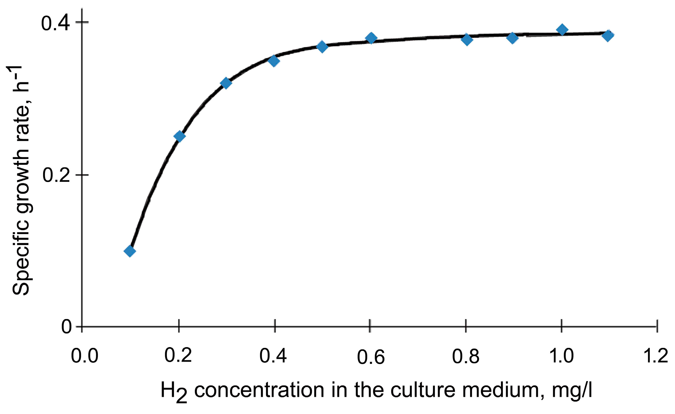
Figure 1. Specific grow rate of Seliberia carboxydohydrogena Z1062 vs. concentration of the limiting H2 dissolved in the culture medium [41].
Mathematics 11 03183 g001
Figure 2. Concentrations of H2 (Mathematics 11 03183 i012, mg/L) and biomass (Mathematics 11 03183 i013, g/L) in Seliberia carboxydohydrogena Z1062 vs. chemostat culture (flow rate 0.15 h−1) as dependent on hydrogen fed into the fermenter (vol.%) [41].
Mathematics 11 03183 g002
Table 1. Different Types of Interactions Providing for Stationary Coexistence of Species in Experimental Flow Systems.
St.
No.
Medium Factors (RFs)Coexisting SpeciesInteraction DiagramRef.
12345
1S, glucose,
P, lactate
X1Lactobacillus plantarum
x2Proptonibacterium shermanii
Mathematics 11 03183 i001[29]
2S, lactate
P, acetate
X1Desulfovibrio desulfuricans
X2Methanobacterium sp.
[30]
3S, manitol
P, fructose
X1Acetobacter suboyxdans
X2Saccharomyces carlsbergensis
[31]
4S, 5-methyl-recorcin (orcin)
P1, unknown product
P2, unknown product
X1Pseudomonas sp.
x2Gram-positive bacilli
x3Gram-positive bacilli
Mathematics 11 03183 i002[32]
5S1PO4 ions
S2SiO2 ions
Diatoms
X1Cyclotello
x2Asterionella
Mathematics 11 03183 i003[33]
6Sparathion (organophosphorus insecticide)
P1paranitrophenol
P2diethyl phosphate
X1Ps. stutzeri
x2Ps. aeruginosa
Mathematics 11 03183 i004[34]
7Soxygen
P1methanol
P2organic matter
P3organic matter
X1Pseudomonas sp.
x2Hyphomicrobium
X3Flavobacterium sp.
X4Acinetobacter sp.
Mathematics 11 03183 i005[35]
8S1noxibenzoate
S2glucose
X1Klebsiella aerogenes
X2Pseudomonas aeruginosa
Mathematics 11 03183 i006[36]
9Sglucose
Priboflavin
X1Saccharomyces cerevisiqe
X2Lactobacillus casei
Mathematics 11 03183 i007[37]
10Sglucose
Pvitamin
X1Candida mycoderma
X2C. tropicalis
[38]
11Sglucose
Punidentified compound
X1Flavobacterium breve (F-39)
X2Fl. ferrugineum (B-21)
Mathematics 11 03183 i008[39]
12S1glucose
S2xylose
x1Candida mycoderma
X2C. tropicalis
Mathematics 11 03183 i009[38]
13S1glucose
S2galactose
X1Candida mycoderma
X2C. tropicalis
[38]
14S1glucose
S2arabinose
X1Candida scottii
X2C. tropicalis
Mathematics 11 03183 i010[38]
15Sglucose
PH+
Saccharomyces cerevisiae:
X1haploid
X2diploid
Mathematics 11 03183 i011[38]
16Ssubstrate
Pinhibitor
Bacteria:
X1inhibitor-insensitive strain
X2sensitive strain
[40]
For example, Diagram 2 means that the substrate, S, makes SGR of the first species ( X 1 ) grow (plus over the arrow), while its own quantity decreases (minus over the reverse arrow); the substance, P, released by species X 1 (plus over the arrow), inhibits growth of the second species ( X 2 ) (minus over the arrow), etc.
Table 2. Characterization of steady states of Candida utilis continuous culture.
State
Number
Sinput, g/LSst, mg/LpHinputpHstXst, mg/LαS, g/gαH, 10−3 M/g
Flow rate 0.1 h−1
1113 ± 22.792.60375 ± 202.63 ± 0.152.37 ± 0.33
2116 ± 44.123.10400 ± 102.45 ±0.131.79 ± 0.07
3120 ± 63.152.79390 ± 252.54 + 0.162.37 ± 0.13
4216 ± 13.142.62840 ± 102.36 ± 0.121.99 ± 0.10
50.57 ± 23.152.89205 ± 102.40 ± 0.102.83 ± 0.34
6112 ± 12.462.32410 ± 102.40 ± 0.133.19 ± 0.43
71.519 ± 42.372.22590 ± 102.51 ± 0.133.02 ± 0.41
8110 ± 22.382.28415 ± 102.38 ± 0.122.59 ± 0.38
9116 ± 42.322.21410 ± 102.41 ± 0.133.38 ± 0.54
10221 ± 42.372.15≥920≤2.15≤2.93
11230 ± 52.232.09945 ± 152.08 ± 0.112.36 ± 0.33
12221 ± 62.182.021070 ± 201.85 ± 0.102.75 ± 0.42
13225 ± 62.142.00980 ± 152.02 ± 0.102.70 ± 0.45
142.548 ± 62.141.901290 ± 201.90 ± 0.102.80 ± 0.58
Flow rate 0.055 h−1
152.558 ± 52.242.101130 ± 302.16 ± 0.061.93 ± 0.21
162.591 ± 102.142.051020 ± 252.36 ± 0.071.67 ± 0.26
17240 ± 52.142.07710 ± 302.30 ±0.101.79 ± 0.37
Indexes “input” and “st” denote the input and steady state values, respectively. X is biomass concentration; αS and αH are coefficients of transformation of glucose and hydrogen ions, respectively, by biomass. pH measurement precision is 0.01 units.
Table 3. SC values for glucose and pH.
Steady StateSinput, g/LpHinputSC for GlucoseSC for pH
1–513.150.00 ± 0.011.10 ± 0.10
6–912.380.02 ± 0.021.06 ± 0.07
7, 10, 1122.370.00 ± 0.010.65 ± 0.10
12–1422.140.05 ± 0.020.71 ± 0.13
13–172.52.140.10 ± 0.030.65 ± 0.20
Disclaimer/Publisher’s Note: The statements, opinions and data contained in all publications are solely those of the individual author(s) and contributor(s) and not of MDPI and/or the editor(s). MDPI and/or the editor(s) disclaim responsibility for any injury to people or property resulting from any ideas, methods, instructions or products referred to in the content.