A GA-Based Scheduling Method for Civil Aircraft Distributed Production with Material Inventory Replenishment Consideration

Abstract

The production of civil aircrafts is confronted with a significant demand for the interconnectivity of production resources among distributed factories, while the complex coupling relationships among various production resources might restrict the improvement of production efficiency. Therefore, researching scheduling methods for civil aircraft distributed production is necessary, but previous studies have not taken material inventory into account sufficiently. This article proposes a scheduling method for civil aircraft distributed production that aims to minimize the production time to complete all the jobs in a large production station under the condition of material inventory replenishment. Firstly, we analyze the factors constraining civil aircraft production efficiency, and formulize the production scheduling problem into the Resource-Constrained Project Scheduling Problem model with Inventory Replenishment (RCPSP-IR). Precedence constraints and resource constraints, especially the inventory constraints, are mainly considered in RCPSP-IR. To solve the corresponding scheduling problem, the Genetic Algorithm (GA) is applied and multiple approaches are introduced to handle the complex constraints and avoid local optimum. Finally, we applied the proposed scheduling method to a case study of a jet twin-engine civil aircraft production of COMAC. The results of the case study show that the proposed method can give a nearly optimal scheduling strategy to be applied to actual civil aircraft production.

1. Introduction

Scheduling methods are still important means to optimize production processes such as [1,2]. This significance is particularly evident in multi-site manufacturing systems [3,4,5]. However, different from the mass production in which the scheduling is simpler and can be described as a disjunctive scheduling problem, the civil aircraft production system is typically a Discrete Manufacturing System (DMS), where the products are assembled from various materials through various production processes. Compared with other manufacturing industries, civil large aircraft production has characteristics, including larger scale, advanced technology, and longer production cycle, requiring a wider variety of resources in the production processes [6]. Furthermore, it is expensive to purchase and stock some of the materials in civil aircraft production. Therefore, it is generally challenging to plan production based on the held material inventory. Instead, the production as well as material consumption is pulled by orders received from customers, typically from airline companies. In other words, the production environment of civil aircraft falls under the category of make-to-order (MTO). The production company must make a long-term production plan according to the received orders. Before the production of a certain flight is commenced, a scheduling scheme must be made in advance. By providing scheduling solutions with shorter production times, it is beneficial to improve production efficiency.

As shown in Figure 1, the civil aviation industry is usually organized on a prime manufacturer–supplier structure, where suppliers are responsible for providing a variety of materials to the prime manufacturer undertaking the final assembly of the aircraft. Since the resources required by the civil aviation production are geographically dispersed, the factories of suppliers are also distributed in different places. Manufacturing companies commonly employ Material Requirements Planning (MRP) for production orders and management. However, MRP may have limitations when applied in the considered civil aircraft production environments. Based on our investigation on the companies, inventory shortages are commonly encountered in the production of the prime manufacturer of civil aircraft, and these shortages usually arise due to the limited production capacity of upstream suppliers. While other production industries can solve this issue by (1) adding more suppliers or (2) requesting suppliers to increase their production capacity, the unique characteristic of civil aircraft production presents challenges in implementing these solutions. The number of aviation suppliers that meet the necessary requirements is often limited, making (1) relatively difficult to achieve. Additionally, the implementation of (2) tends to be slow for aircraft production. As a result, it is necessary to schedule under the limited inventory.

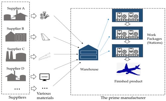
Figure 1. A diagram of the layout of the distributed manufacturing of civil aircraft.

By conducting on-site investigation, we conducted a comprehensive analysis of the factors that could affect civil aircraft production efficiency and discover that the factors constraining the production time mainly come from two aspects: precedence constraints and resource constraints. Precedence constraints include the certain time required for each production operation to complete, and the precedence relationship between each production operations, which can be represented by a directed acyclic graph in the form of activity-on-node (AON). Resource constraints are usually reflected in the limited amount of materials required for each production operation. Taking into consideration the existence of these two aspects of constraints and the distributed characteristic of civil aircraft manufacturing, the production activities of the work packages in aircraft production can be modeled by Resource-Constrained Project Scheduling Problem (RCPSP).

RCPSP and its variants have been widely practiced already in describing industrial scheduling problems, including civil aviation production in recent years. For example, ref. [7] described an aircraft assembly scheduling problem using RCPSP, and attempted to solve it using two different coding methods based on a demand-driven GA. However, the types of resource it mainly considered were reusable human resources, with limited consideration on material inventory. Ref. [8] described the paced aircraft assembly line rescheduling problem as an RCPSP, and proposed novel optimization criteria suitable for the aircraft manufacturing environment. However, the material resources were mainly not replenishable. Considering the situation where there were multiple stations sharing resources in an aircraft moving assembly line, ref. [9] proposed a resource investment problem based on project splitting with time windows and a two-stage iterative loop algorithm was used to solve the corresponding optimization problem. The unpredictability of resource shortages was also considered, but its application scenario did not include material inventory.

The above examples of research on scheduling aircraft production with RCPSP modeling have insufficient consideration on inventory. In their models, the materials are not replenishable and limited by the application scenarios. In practical production, the material inventory would fluctuate rather than strictly being renewable or unrenewable during the production process, because of the continuous supply from upstream suppliers. We stress the importance of considering replenishable material because civil aircraft production enterprises are prone to production delays caused by inventory shortages in practical production. The shortages are usually caused by inflexible scheduling strategy.

Considering that the consumption of the material inventory is driven by orders, it is necessary to model the replenishable material inventory. Since the production capacity of the upstream suppliers is limited, it is unrealistic to stock all the required materials in advance when an order occurs. From the scheduler’s point of view, the material inventory is supplied periodically, and different processes may potentially compete for materials. Thus, it is necessary to consider the production as an RCPSP-IR.

In this article, we propose a GA-based scheduling method for civil aircraft distributed production, taking into consideration material inventory replenishment. First, we formulate the civil aircraft production scheduling problem as an RCPSP-IR. By analyzing the production process, we formulate the problem into a mixed integer programming (MIP) problem. Then, we introduce GA with resource constraints to solve RCPSP-IR so as to minimize the production time. To deal with the complex constraints including the inventory constraints, different constraint handling approaches and local optima preventing methods are used. Finally, to evaluate effectiveness of the proposed scheduling method, we conduct a case study of a jet twin-engine civil aircraft production of COMAC. The results of the case study show that the proposed method can give a nearly optimal scheduling strategy to be applied to actual civil aircraft product919ion.

The remainder of this paper is organized as follows:

Section 2 introduced the related work; In Section 3, the aircraft production process is summarized and the corresponding mathematical model of RCPSP-IR is described; In Section 4, the model is solved by GA considering the complex constraints; Section 5 gives the computational result of a case study; Finally, Section 7 summarizes the paper.

2. Related Work

2.1. Variants of RCPSP on Different Resources Consideration

Project scheduling problems are a large class of problems researching how to balance the overall cost or completion time in a project by solving the decision problem of resource allocation. According to [10], as one type of project scheduling problem, the characteristic of RCPSP is that there are mainly two interdependencies among the activities. First, the activities need to compete for limited resources that are required to conduct activities. Second, there are precedence constraints between the activities, which means each pair of adjacent activities must be conducted in a predetermined order. RCPSP belongs to the category of NP-hard problems.

Although RCPSP already has a formalized description and widely applied in a variety of problems, its original form cannot cover all practical scenarios, especially the scenarios with more complex resource considerations. The traditional RCPSP assume that the amount of all resources is given at the beginning and is not replenishable as the activities process. Therefore, in recent years, some studies have proposed different modifications to RCPSP based on the characteristics of resource for specific problems. For example, in multi-mode RCPSP (MRCPSP), resources can be divided into renewable resources that are occupied when being used and can be reused by other activities after being released, and unrenewable resources that would be consumed in quantity [11]. In [12], the scheduling problem of dismantling activities as an MRCPSP with cumulative resources was explored. Article [13,14] considered the scenario where the resource request would change from time to time. Reference [15] considered time-dependent resource requests within a problem setting that includes multiple skills. In [16], the scenario where the overall budget of the project should be allocated to different types of resource to determine the general resource capacity corresponding to the total amount of renewable resources to be allocated specifically to the project was considered, and the project manager should allocate resources to each project based on overall resource capacity. An integrated model was built, and two solution methods—a two-stage method and a GA method—were proposed.

2.2. Existing RCPSP Applications Considering Inventory

There have already been some examples of research considering the material inventory factors in other areas. For instance, driven by the limited inventory capacity, reference [17] proposed a model for an MRCPSP scenario where the maximum total resource capacity was limited. Their proposed model for railway construction projects included activity scheduling, material ordering, and supplier selection. For material ordering, different supplier discounts and inventory costs were taken into account. Reference [18] also considered the inventory problem. On the basis of the RCPSP, the interval-valued fuzzy number was additionally introduced to model the uncertainty in the project, and a mixed multi-objective method was proposed to solve the interval valued-fuzzy mathematical model. Aiming at the trade-off between the cost and environmental impact of the project and considering the inventory procurement, reference [19] proposed a mixed integer programming model based on RCPSP. In addition, in [20], a hybrid scheduling problem was proposed. It considered the objective of minimizing the makespan of the project as well as maximizing the robustness and minimizing the total cost caused by material ordering. Reference [21] integrated MRCPSP and material batch ordering for a construction project; a hybrid algorithm was proposed to solve it.

In summary, although there have been studies on RCPSP considering inventory factors in various domains, the practice of RCPSP specifically on civil aircraft production still needs further exploration. We believe the following research gaps exist: Although in many areas there have been studies on RCPSP that consider inventory factors, the consideration on inventory is not enough when RCPSP is applied on civil aircraft production. The RCPSP-IR in this paper will be dedicated to solving the problem, and we are going to provide a mathematical formulation for practical production problems, and then apply optimization algorithms on its computational experiments.

3. RCPSP-IR Modeling for the Distributed Production Scheduling of Civil Aircraft

3.1. Introduction of Civil Aircraft Production Process

The manufacturing of civil aircrafts is a typical DMS where its production process can be decomposed into many processing tasks to complete. Its production consists of several large, isolated work packages. These work packages are completed by stations on the actual production line. The production efficiency of those stations on the main production line directly affects the total aircraft production time. These stations include the installation and docking of the front, middle, and rear sections of the fuselage, as well as the assembly of the front and rear wings. The large work packages can be further divided into sub work packages, corresponding to the substations inside the station as shown in Figure 2. The substations involve many working procedures. It takes a certain amount of time and consumes a certain quantity of materials including structural parts, standard parts, and raw materials to carry out a procedure, and if the work package’s production design does not change, its consumption quantity usually does not change greatly.

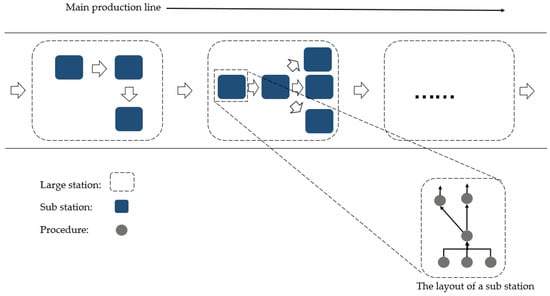
Figure 2. The diagram of the relationship among stations and procedures. At the top level, the main production line of the prime manufacturer is made up of various stations, and each station is composed of a series of substations. The minimum scale in our consideration is procedure shown by gray circles. All stations, and procedures at their level have certain procedure relationships.

There exists a precedence relationship between the procedures, where each certain procedure can only start after its predecessor procedures have all been completed. Each procedure progresses according to this order, until the final procedure is conducted. By regarding each procedure as a node and the temporal precedence relationship between them as an edge, we can represent the precedence relationship as an Activity-on-Node (AON) structured graph as shown in Figure 3. In the AON graph, a node is connected to the nodes representing its predecessor procedures through the incoming edges, and the outgoing edges are linked to the nodes representing its successor procedures. All paths in the graph do not always lead to the same final node, which represents a branch that occurs in the production process. The overall graph is a directed acyclic graph (DAG) for there is no cycle in the production, and the graph must be a connected graph.

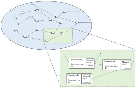
Figure 3. A part of the AON graph representing the production. Each procedure node has two main attributions—processing time and required materials.

In addition to the precedence relationship mentioned above, inventory is also a major factor restricting the production. It is worth noting that the materials required by each procedure is listed by its technological document. Before the procedure is started, all materials required must be available and transported from the inventory to the shop. The types and numbers of these materials would be checked. Only after that, the procedure can begin. All these materials are stored in the warehouse of the prime manufacturer. These materials mainly come from the orders from upstream suppliers. Generally, according to the technological document, a procedure requires several types of materials, and the amount of each type of material required is different. Both the types and amount required would be different among the procedures. The inventory replenishment periods and replenishment quantities for each type of material are also different. Materials with low complexity and technology such as standard parts and raw materials have large output and can be produced and supplemented at a stable rate, while the structural parts produced by strategic suppliers have limited output and longer replenishment cycle.

From the above, it can be seen that for the prime manufacturer, the production capacity is constrained by the capacity of stations on the main line, and the factors restricting the capacity of stations mainly come from two aspects: (1) precedence constraints; (2) resource constraints. In terms of precedence constraints, each procedure needs a certain amount of time to complete, and the execution of each procedure requires the completion of some other procedures as a precondition.

The factors of resource constraints should be emphasized. In terms of resource constraints, each procedure consumes a certain type and quantity of materials. Restricted by the limited production capacity of upstream suppliers and the consumption by production, the main manufacturer may not have enough materials in the inventory to simultaneously conduct all procedures that meet time constraints. On the other hand, some procedures may require the same types of material, which will inevitably lead to the competition among procedures for materials. Because of these two aspects of constraints, the scheduling solution needs to be responsible for both the procedure scheduling and resource scheduling.

These two aspects of constraints make the problem fit the characteristics of RCPSP, and the production activities in the stations can be modeled in the framework of RCPSP. Additionally, compared with the classic RCPSP, the replenishable inventory should be considered, because the total amount of resources in many RCPSP models are initially given at the beginning of the project and are renewable as the project processes. The main difference between our aircraft production problem and traditional RCPSPs is that the inventory of material can be replenished by upstream suppliers and consumed by the procedures over time. Therefore, it should be defined as an RCPSP with inventory replenishment (RCPSP-IR). Table 1 compares difference between RCPSP and our model considering inventory constraints.

Table 1. Comparison of RCPSP and RCPSP-IR.

RCPSP	RCPSP-IR
Model input does not include material inventory replenishment and consumption.	Model input includes material inventory replenishment and consumption.
Poor ability to describe situations where inventory is insufficient.	Can describe the situation of insufficient inventory. Making it possible to efficiently schedule production.

3.2. Formulization of RCPSP-IR

Considering that civil aircraft production is DMS, we assume the whole production process is decomposed into many stations and procedures, and the precedence relationship of the procedures in a station can be represented by a connected AON which is a DAG. In addition, the aircraft production environment is MTO, and inventory is limited by the amount and period of material supplied by upstream suppliers. So, the production plan must be scheduled in advance because of the inventory constraints for a specific production link. According to the historical inventory data, we assume that upstream suppliers and manufacturing departments provide materials regularly and quantitatively.

On the basis of the production process, the following assumptions are made to solve and verify the model:

• Upstream suppliers and manufacturing departments provide materials regularly and quantitatively;
• Each type of material has its own supply quantity and supply cycle;
• The whole production process of a civil aircraft can be decomposed into many procedures;
• Each procedure must only be started after the completion of its predecessor procedure, and takes a certain amount of time to complete;
• No cycle during the production. In other words, the AON graph is a DAG;
• The AON graph is a connected graph;
• Supply disruptions or production breakdown caused by external factors, like quality issues, human error, and sudden fault, are not considered;
• Working hour is the time unit of this model.

In this article, the scheduling problem of civil aircraft production is solved through the idea of optimization. The objective of the established optimization model is to minimize the overall production time of each station. The decision variable is the start time of each procedure. As previously mentioned, time factors and resource factors, including inventory, are mainly considered. The variables related to time factors should include the procedure precedence constraints and execution time, etc. The variables related to resource factors encompass the quantity of materials required for each procedure, as well as the inventory replenishment quantities and periods. Since the procedures and material consumption are closely coupled, scheduling material resources can also be achieved by scheduling the start time of the procedures. Depending on the replenishment quantities and periods, three kinds of materials are considered: raw materials, standard parts, and structural parts. The symbols and their definitions appearing in this paper are shown in Table 2, including the symbols related to GA used in this article.

Table 2. Notations and explanations.

	Symbol	Definition
Sets	$D_S$	Set of structural parts
	$D_P$	Set of standard parts
	$D_W$	Set of raw materials
	$D_I$	Set of the procedures
Notations	$s,p,w$	Numbers of materials, $s\in D_S,p\in D_P,f\in D_w$
	$i$	Numbers of procedure $i$ in the station, $i\in D_I$
	$t$	The $t$ th hour during the production process
	$\tau$	A solution of the problem
Parameters of the problem	$N_s\left(t\right),N_p\left(t\right),N_w^{}\left(t\right)$	The inventory quantity of material $s$(or $p$, $w$) at the hour $t$
	$Y_s^{}{,Y}_p^{},Y_w^{}$	The inventory replenishment quantity of material $s$(or $p$, $w$) per time
	$I_s^{},I_p^{}{,I}_w^{}$	Inventory replenishment period of material $s$(or $p$, $w$)
	${MP}_i^{}$	Time needed for procedure $i$ to finish
	$S_i^{}\left(s\right),P_i^{}\left(p\right),W_i^{}\left(w\right)$	Amount of materialrequired to start procedure $i$
Variables	${ST}_i^{}$	Decision variables. The start time of procedure $i$
	${CL}_i^{}$	The completion time of procedure $i$
	$\Delta t_i^{}$	Time difference between ${ST}_i^{}$ and the latest completion time of $i$‘s pre-procedure
	$R_s\left(t\right),R_p\left(t\right),R_w\left(t\right)$	Boolean value describing whether material is replenished at $t$
	$B_i^{}\left(t\right)$	Boolean value describing whether procedure $i$ starts at $t$
	$G_s\left(t\right),G_p\left(t\right),G_w^{}\left(t\right)$	The inventory constraint violation value of material $s$(or $p$, $w$) at $t$
Symbols related to GA	$v\left(\tau \right)$	Violation of constraints by solution $\tau$
	$f\left(\tau \right)$	Fitness function of solution $\tau$
	$P$	The population of GA
	$r\left(P\right)$	The proportion of feasible solutions in population $P$
	$g$	The generation of GA.
	$m$	Number of resource constraint inequalities
	$c,d,\alpha ,\beta$	Constant values
	$e$	Extinction countdown
	$T_{}$	The time objective function
	$T_{}=\mathrm{m}\mathrm{a}\mathrm{x}\left\{{CL}_i^{}\right\}$	Objective equals to the end time of the last completed task

The constraints presented in the form of equations and inequalities are as follows.

In our consideration, the whole production process starts at time 0 so all variables representing time should be non-negative. For all $i$,

$${ST}_i^{}\ge 0$$

(1)

$${CL}_i^{}\ge 0$$

(2)

The precedence constraints contain a series of inequalities, stating that only after all the predecessors are finished can a procedure start. “$SC\left(i^{\prime }\right)=i$” represents that the succeed procedure of procedure $i^{\prime }$ is procedure $i$.

$${ST}_i^{}\ge {{CL}_{i^{\prime }},}_{}^{}\mathrm{for}\mathrm{all}SC\left(i^{\prime }\right)=i$$

(3)

According to the definition of ${MP}_i^{}$ we have the following:

$${CL}_i^{}={ST}_i^{}+{MP}_i^{}$$

(4)

By combining the previous Formulas (4) and (5), we have the following:

$${ST}_i^{}\ge {\underset{i^{\prime }}{\max (}{\mathit{ST}}_{i^{\prime }}^{}+{\mathit{MP}}_i^{}),{}_{{}^{}}^{}}_{}^{}\mathrm{for}\mathrm{all}SC\left(i^{\prime }\right)=i$$

(5)

The current inventory depends on the delivery volume from suppliers and consume volume caused by the production activities. Taking structural part $s$ for example (the situation for raw materials and standard parts are the same),

$$N_s^{}\left(t+1\right)=N_s^{}\left(t\right)+R_s\left(t\right)·Y_s^{}-B_i^{}(t)·{\sum }_i^{t={CL}_i^{}}{S}_i^{}\left(s\right)$$

(6)

Here, $R_s\left(t\right)$ and $B_i^{}\left(t\right)$ are the Boolean functions, respectively describing whether there is inventory replenishment of part $s$ happening at moment $t$, and whether procedure $i$ starts at moment $t$:

$$B_i^{}(t)=\left\{\begin{array}{c}1,\mathrm{if}t={ST}_i^{},\hfill \\ 0,\mathrm{if}t\ne {ST}_i^{}\hfill \end{array}\right.,$$

(7)

The value of $R_s\left(t\right)$ depends on the order strategy of the factory and in our assumption so there should be a time sequence ${LT}_s^{}=[l_s^0,l_s^1,l_s^2,l_s^3,\dots ]$ indicating the date list when there are parts arriving. As mentioned above, we assume here that they arrive at constant intervals, so $R_s\left(t\right)$ represents whether $t$ is in ${LT}_s^{}$.

In the AON representing the manufacturing process, there is no acyclic, so every job should and can only be conducted once. For a pair of fixed $w$ and $i$,

$$\sum _t{B}_i^{}\left(t\right)=1,$$

(8)

The inventory of each kind of material should have a lower bound, or at least it should not be a negative value. The lower bound can be fixed to another value if it is necessary to set a safety inventory. In the following case study, we set the lower bound of inventory to 0 and directly consider the relative value of the current inventory compared to the safety inventory.

$$N_s^{}\left(t\right)\ge 0,\hspace{1em}\hspace{1em}\mathrm{for}\mathrm{all}t,s$$

(9)

4. RCPSP-IR Solving Based on GA

The main challenge to solve RCPSP-IR by GA is how to deal with the constraints associated with the problem. The scale of the problem and the complexity of the constraints seriously restrict the efficiency of computation. There is a large number of constraints in the model. Firstly, precedence constraints exist between two adjacent procedures. Secondly, at every moment there is an inventory lower bound constraint for each type of material. Moreover, there is a strong coupling relationship among these constraints, making the feasible region quite narrow. If GA is left to evolve and iterate from random population without intervention, it may not reach the feasible region in acceptable runtime, let alone find a feasible optimal solution. Thus, the two aspects of constraints need to be handled accordingly.

4.1. Precedence Constraints

Precedence constraints can be solved by variable substitutions. The precedence constraints are easily violated because it is hard to generate a scheduling policy satisfying the constraint between a pair of procedures without violating the others. Since the GA does not strictly impose requirement on whether the optimization problem is linear or not, inequality (3) can be transformed into (10):

$${ST}_i^{}\ge {\underset{i^{\prime }}{\max }{\mathit{CL}}_{i^{\prime }},}_{}^{}\mathrm{for}\mathrm{all}SC\left(i^{\prime }\right)=i^{}$$

(10)

The inequalities can then be translated into equalities to reduce the difficulty of solving by introducing variable $\mathsf{\Delta }{t}_i^{}$ as shown in (11) and (12). The main decision object $\tau$ becomes the array composed of $\mathsf{\Delta }{t}_i^{}$ for each procedure $i^{}$ as shown in (13).

$${ST}_i^{}=\Delta t_i^{}+{\underset{i^{\prime }}{\max }{\mathit{CL}}_{i^{\prime }}^{}}_{}^{}$$

(11)

$$\Delta t_i^{}\ge 0$$

(12)

$$\tau =[\Delta t_1^{},\Delta t_2^{},\Delta t_3^{},\dots ]$$

(13)

4.2. Resource Constraints Considering Inventory Replenishment

For the resource constraints, the inventory fluctuates every moment and cannot be easily eliminated. Generally, when solving combinatorial optimization problems, GA often employs the penalty method and the correction algorithm to handle constraints. Since the correction algorithm depends on specially designed heuristics for complex problems, it is not as concise and flexible as the penalty function method while they achieve similar effects. So, the penalty function method applied to solve the inventory constraints. The penalty method generally adds a penalty function term $v\left(\tau \right)$ to solutions that violate the constraints in order to reduce their fitness, so that they are less fit and easier to be eliminated during the iteration. $v\left(\tau \right)$ represents the degree of constraint violation by solution $\tau$, and its value depends on the selected penalty method.

It should be noted that the feasible regions of different problems have different characteristics, and there is no universal penalty function that can be applied. In addition, some penalty functions also involve coefficient adjustment such as static penalty, and the performance of the penalty functions may also be related to the hyperparameter configuration of GA, so it is necessary to compare experiments to find a penalty function that can deal with the constraints of the problem in this paper. Three penalty function methods are potentially helpful in handling these complex constraints.

$$f\left(\tau \right)=T\left(\tau \right)+v\left(\tau \right)$$

(14)

4.2.1. Static Penalty

In our consideration, since the inventory quantity has a lower bound, the inventory constraint violation term of a certain material at a specific time should be defined as (15). In the static penalty method (denoted by SP), the total constraint violation $v\left(\tau \right)$ is the weighted sum of violations of all constraint terms shown in (16), where $\beta$, $c_{s,t}$are constant values and $\beta$ can be 1 or 2, similar to the method mentioned in [22]. Obviously, results of SP will be influenced by the values of these constant coefficients.

$$G_s\left(t\right)=\left\{\begin{array}{c}-N_s\left(t\right),N_s\left(t\right)<0\hfill \\ 0,N_s\left(t\right)\ge 0\hfill \end{array}\right.$$

(15)

$$v\left(\tau \right)=\sum _{s,t}^{}{c}_{s,t}(G_s\left(t\right){)}^{\beta }+\sum _{p,t}^{}{c}_{p,t}(G_p\left(t\right){)}^{\beta }+\sum _{w,t}^{}{c}_{w,t}(G_w\left(t\right){)}^{\beta }$$

(16)

4.2.2. Dynamic Penalty

In the dynamic penalty method (denoted by DP), the violation coefficient values depend on the current iteration of GA, as shown in (17), where $C,\alpha ,\beta$ are constant, and $g$ is the current iteration. In this way, a larger penalty can be imposed on infeasible solutions when the number of iteration rounds is relatively large, and theoretically it is expected to avoid the algorithm from making too many useless explorations in the infeasible domain.

$$v\left(\tau \right)={\left(C\ast g\right)}^{\alpha }\ast (\sum _{s,t}^{}(G_s\left(t\right){)}^{\beta }+\sum _{p,t}^{}(G_p\left(t\right){)}^{\beta }+\sum _{w,t}^{}(G_w\left(t\right){)}^{\beta })$$

(17)

4.2.3. Adaptive Penalty

We adopt two adaptive penalty methods for potentially better algorithm performance. In the first adaptive penalty method (denoted by AP1), the factor of penalty term is computed dynamically according to the individuals in the population at the current generation. As shown in (18) and (19), theoretically it is expected to automatically expand its search range if the past k generations are all feasible and narrowing its search area to obtain a feasible solution if the past k generation are not feasible, same as [22].

$$v\left(\tau \right)=\lambda \left(g\right)·(\sum _{s,t}^{}{G}_s\left(t\right)+\sum _{p,t}^{}{G}_p\left(t\right)+\sum _{w,t}^{}{G}_w\left(t\right))$$

(18)

$$\lambda \left(g+1\right)\left\{\begin{array}{c}\frac{1}{{\beta }_1}·\lambda \left(g\right),\mathrm{The}\mathrm{optimal}\mathrm{solutions}\mathrm{in}\mathrm{the}\mathrm{past}k\mathrm{generations}\mathrm{are}\mathrm{all}\mathrm{feasible}\hfill \\ {\beta }_2·\lambda \left(g\right),\mathrm{None}\mathrm{of}\mathrm{the}\mathrm{optimal}\mathrm{solutions}\mathrm{in}\mathrm{the}\mathrm{past}k\mathrm{generations}\mathrm{is}\mathrm{feasible}\hfill \\ \lambda \left(g\right),\mathrm{Otherwise}\hfill \end{array}\right.$$

(19)

Different from the method above, the second penalty adaptive method (denoted by AP2) normalized the objective function of populations and constraint violations of individuals separately. Similar with [23], when there were fewer feasible solutions in the population, the weight of the penalty for violating the constraints is increased to obtain more feasible solutions. When there are more feasible solutions, the weight of the optimization goal is increased to obtain the optimal solution. Where $\tilde{T}\left(\tau \right)$ is the normalized optimization goal, $v\left(\tau \right)$ is the normalized violation of the individual, and $r\left(P\right)$ is the proportion of feasible solutions in $P$.

$$f\left(\tau \right)=\left\{\begin{array}{c}\tilde{T}\left(\tau \right),\mathrm{for}\mathrm{feasible}\mathrm{individual}\\ v\left(\tau \right),\mathrm{if}\mathrm{there}\mathrm{is}\mathrm{no}\mathrm{feasible}\mathrm{individual}\\ \sqrt{{\tilde{T}}^2\left(\tau \right)+v^2\left(\tau \right)}+r\left(P\right)\ast \tilde{T}\left(\tau \right)+\left(1-r\left(P\right)\right)\ast v\left(\tau \right),\mathrm{otherwise}\end{array}\right.$$

(20)

$$\tilde{T}\left(\tau \right)=\frac{T\left(\tau \right)-\underset{\mathit{\tau \; in\; P}}{\min }T\left(\tau \right)}{\underset{\mathit{\tau \; in\; P}}{\max }T\left(\tau \right)-\underset{\mathit{\tau \; in\; P}}{\min }T\left(\tau \right)}$$

(21)

$$v\left(\tau \right)=\frac{1}{m}\ast \frac{1}{\underset{s,t}{\max }{G}_s\left(t\right)}\mathrm{*}(\sum _{s,t}^{}{G}_s\left(t\right)+\sum _{p,t}^{}{G}_p\left(t\right)+\sum _{w,t}^{}{G}_w\left(t\right))$$

(22)

4.3. Prevention of Local Optima

Another concern is the local optima resulting from premature convergence, which is quite common when applying GA. According to [24], although it is hard to totally avoid falling into local optima and verify the current optimal solution’s optimality, increasing the individual diversity of the population is still useful to reduce local optima. This can be achieved by properly increasing the crossover rate or mutate rate and increasing the magnitude of mutation.

One of the characteristics of our problem is that the feasible regions are distributed in isolation if the range of the optimization goal is restricted. Some penalty methods, such as DP and AP1, trend to assign a large penalty to the infeasible individuals, which would lead the individuals to fall into a nearby feasible region where there is no optimal solution in a hurry.

An extinction mechanism is introduced to solve local optima. If the optimal feasible solution is not being improved for $e$ generations, where $e$ is the countdown, all optimal feasible individuals would be removed from the population and replaced by randomly generated new individuals, because that potentially means it may be trapped in a local optimum.

By adopting the methods above, the algorithm can be expressed as Algorithm 1.

Algorithm 1 Overview of GA in this article
1:	Define the selection mechanism, the crossover mechanism, the mutation mechanism.
2:	Define the extinction countdown $e$.
3:	Initialize the population P and maximum iteration episodes $g_{max}$.
4:	For each individual $\tau$ in $P$, calculate the fitness $f\left(\tau \right)$.
5:	for $g=0\to g_{max}$:
	(a)	Select from $P$ to obtain a new population $P^{\prime }$ according to the selection mechanism.
	(b)	for each pair of individuals ${\tau }_1,{\tau }_2$ in $P^{\prime }$, with a crossover probability:   Crossover ${\tau }_1,{\tau }_2$ to obtain offspring ${\tau }_1\prime ,{\tau }_2\prime$ according to the crossover mechanism.   Replace ${\tau }_1,{\tau }_2$ with ${\tau }_1\prime ,{\tau }_2\prime$. end for
	(c)	for each individual $\tau$ in $P^{\prime }$, with a mutation probability:   Mutate $\tau$ to get solution$\tau \prime$ according to the mutation mechanism   Replace $\tau$ with $\tau \prime$. end for
	(d)	Recalculate the fitness $f\left(\tau \right)$ of each individual $\tau$ in $P^{\prime }$.
	(e)	Obtain the current optimal feasible solution from $P^{\prime }$. If the fitness of the current optimal feasible solution is not getting improved for $e$ generations, remove all optimal feasible individuals from $P^{\prime }$, and recalculate the fitness $f\left(\tau \right)$ of each individual $\tau$ in $P^{\prime }$.
	(f)	Replace $P$ with $P^{\prime }$.
	end for
6:	Return the optimal feasible solution O in population P.

5. Case Study and Analysis

5.1. Case Discription

In this section, we present a real case study in a jet twin-engine civil aircraft production of COMAC to demonstrate the feasibility and practicality of the presented model in real-world scenarios. In the case, we specifically focus on a station involving fuselage docking on the main production line. The station comprises in total 134 procedures and requires around 17 kinds of materials. The information of the materials including their replenishment period and quantity are shown in Table 3. Note that these 17 raw materials are not all the materials required by the station. Some materials that are in high supply and not prone to shortages are not considered. These procedures belong to nine substations. The precedence relationship of these nine substations is shown in the Figure 4, covering the installation procedures, testing, and checkout before entering storage. Additional information of the substations is shown in Table 4, Table 5, Table 6, Table 7, Table 8, Table 9, Table 10, Table 11 and Table 12. Although the duration of each procedure may vary due to technical improvements, within the production process of a single aircraft, each procedure is executed only once. In the event of any changes to the procedure, a new plan will be rescheduled accordingly.

Table 3. Information about the materials.

Material Identifier	Category	Replenishment Period (h)	Replenishment Quantity
C01	structural part	100	1
C02	structural part	20	4
E01	structural part	80	3
F01	structural part	80	2
H01	structural part	203	1
H02	structural part	15	5
H03	structural part	237	1
H04	standard part	100	100
J01	standard part	400	30
M01	standard part	2	2
R01	structural part	408	1
S01	standard part	75	8
S02	raw material	10	154
X01	standard part	9	54
X02	standard part	70	12
B01	raw material	2	1200
A01	structural part	165	1

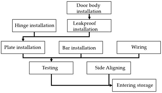
Figure 4. Precedence relationship of the substations.

Table 4. The procedures in the substation of door body installation.

Procedure	Predecessor Procedures	Duration (h)	Required Material Type and Amount
PD1	PD2	11	None
PD2	PD3, PD4, PD5, PD6, PD7, PD8, PD9, PD10, PD11	15	F01(7), S02(14), X01(13), X02(8), B01(2400)
PD3	None	18	E01(2), S02(16), X01(2), X02(9), B01(3323)
PD4	None	5	X01(2), B01(2564)
PD5	None	1	F01(7), S02(27), X01(13), X02(8), B01(2425)
PD6	None	3	E01(2), S02(15), X01(2), X02(9), B01(2747)
PD7	None	1	X01(2), B01(2397)
PD8	None	9	S02(1), X01(2), X02(2), B01(133)
PD9	None	7	None
PD10	None	14	S02(1), X01(2), X02(2), B01(133)
PD11	None	11	None
PD12	PD13	27	S02(10), B01(11,400)
PD13	PD14, PD15, PD16, PD17, PD18, PD19, PD20, PD21	6	B01(1820)
PD14	None	22	B01(3000)
PD15	None	9	B01(12,533)
PD16	None	13	None
PD17	None	5	B01(760)
PD18	None	5	B01(2403)
PD19	None	15	B01(2204)
PD20	None	13	B01(2608)
PD21	None	8	B01(200)

Table 5. The procedures in the substation of leakproof installation.

Procedure	Predecessor Procedures	Duration (h)	Required Material Type and Amount
PL1	PD2	27	X01(60), B01(712)
PL2	PL3, PL4, PL5, PL6, PL7, PL8, PL9	13	None
PL3	PD2, PD13	13	None
PL4	None	17	None
PL5	None	21	F01(7), S02(27), X01(13), X02(8), B01(2425)
PL6	None	32	E01(2), S02(15), X01(2), X02(9), B01(2747)
PL7	None	16	X01(2), B01(2397)
PL8	None	31	S02(1), X01(2), X02(2), B01(133)
PL9	None	31	None

Table 6. The procedures in the substation of hinge installation.

Procedure	Predecessor Procedures	Duration (h)	Required Material Type and Amount
PH1	PH2	36	None
PH2	PH3, PH4, PH5	21	H04(153), J01(1), B01(6832)
PH3	None	23	B01(14,374)
PH4	None	1	H04(408)
PH5	None	8	H04(5), S01(1)
PH6	PH7	19	None
PH7	PH8, PH9, PH10, PH11	36	C02(7), B01(20,000)
PH8	None	21	S02(25), B01(9589)
PH9	None	23	B01(3624)
PH10	None	1	C02(6), H02(4), S02(4), B01(2900)
PH11	None	4	J01(3), B01(3200)

Table 7. The procedures in the substation of plate installation.

Procedure	Predecessor Procedures	Duration (h)	Required Material Type and Amount
PP1	PH2	23	None
PP2	PP3, PP4, PP5, PP6, PP7, PP8, PP9	14	M01(247), B01(3600)
PP3	PL2, PH2, PH7	21	M01(188), B01(3652)
PP4	None	31	B01(5972)
PP5	None	18	B01(6668), A01(2)
PP6	None	27	B01(560)
PP7	None	18	None
PP8	None	19	None
PP9	None	15	B01(160)
PP10	PP11	18	C02(14), H04(55), B01(93)
PP11	PP12, PP13, PP14, PP15, PP16, PP17	27	C02(149), H04(54), B01(5755)
PP12	PP2	18	H04(8), B01(9)
PP13	None	19	H02(12), H04(20), X01(11), B01(999)
PP14	None	15	C02(4), H04(369), J01(40), B01(5000)
PP15	None	13	H04(4), X01(10), B01(7980)
PP16	None	4	H04(18), X01(36), B01(6374)
PP17	None	5	C02(1), H04(1)

Table 8. The procedures in the substation of bar installation.

Procedure	Predecessor Procedures	Duration (h)	Required Material Type and Amount
PB1	PB2	13	None
PB2	PB3, PB4	17	B01(241)
PB3	None	5	S02(7), B01(1130)
PB4	None	5	S01(1), B01(12)

Table 9. The procedures in the substation of wiring.

Procedure	Predecessor Procedures	Duration (h)	Required Material Type and Amount
PW1	PW2	18	None
PW2	PW3, PW4, PW5, PW6, PW7, PW8, PW9	15	F01(7), S02(14), X01(13), X02(8), B01(2400)
PW3	None	15	E01(2), S02(16), X01(2), X02(9), B01(3323)
PW4	None	8	X01(2), B01(2564)
PW5	None	6	F01(7), S02(27), X01(13), X02(8), B01(2425)
PW6	None	6	E01(2), S02(15), X01(2), X02(9), B01(2747)
PW7	None	1	X01(2), B01(2397)
PW8	None	9	S02(1), X01(2), X02(2), B01(133)
PW9	None	14	None
PW10	PW11	5	B01(30)
PW11	None	5	B01(5402)

Table 10. The procedures in the substation of side aligning.

Procedure	Predecessor Procedures	Duration (h)	Required Material Type and Amount
PS1	None	13	B01(348)

Table 11. The procedures in the substation of testing.

Procedure	Predecessor Procedures	Duration (h)	Required Material Type and Amount
PT1	PD2	31	None
PT2	PT3, PT4, PT5, PT6, PT7, PT8, PT9, PT10, PT11, PT12, PT13, PT14, PT15	19	H01(4), S02(1), X01(10), B01(3700)
PT3	PP11, PW2, PW11, PB2	23	C02(5), B01(151)
PT4	None	14	C02(2), B01(883)
PT5	None	21	S01(52), B01(1080)
PT6	None	31	X01(51), X02(26), B01(1500)
PT7	None	18	H02(29), X01(38), B01(2995)
PT8	None	27	S01(10), S02(4), B01(315)
PT9	None	18	S02(2), B01(438)
PT10	None	19	C01(8), S01(8), B01(1274)
PT11	None	15	C01(1), B01(1484)
PT12	None	13	X01(51), X02(14), B01(4756)
PT13	None	4	X01(28), B01(16)
PT14	None	5	X01(2), B01(16)
PT15	None	12	S01(4), B01(197)
PT16	PT17	25	None
PT17	PT18, PT19, PT20, PT21, PT22, PT23, PT24, PT25	23	B01(61)
PT18	PT2	19	None
PT19	None	36	S01(4), X01(1), B01(5300)
PT20	None	21	H02(232), H03(3), H04(21), X01(41), B01(9500)
PT21	None	23	X01(4), B01(7900)
PT22	None	1	None
PT23	None	8	B01(4300)
PT24	None	21	S02(2), B01(1869), A01(3)
PT25	None	6	B01(64)
PT26	PT27	15	S02(28), B01(20,000)
PT27	PT28, PT29, PT30	27	S02(127), B01(20,000)
PT28	PT17	13	S02(15), B01(7274)
PT29	None	13	S02(1), B01(1590)
PT30	None	17	M01(8), S02(14,000)
PT31	PT32	21	H02(20), B01(12,400)
PT32	PT33, PT34, PT35	32	E01(10), B01(4400)
PT33	PT27	16	E01(19), B01(4000)
PT34	None	31	B01(3300)
PT35	None	31	B01(3600)
PT36	PT37	11	B01(19)
PT37	PT38, PT39, PT40	25	H02(1), B01(33,000)
PT38	PT32	26	C02(33), R01(1), B01(2800)
PT39	None	29	B01(2168)
PT40	None	14	C02(8), B01(115)
PT41	PT42	21	B01(20)
PT42	PT43, PT44, PT45	14	None
PT43	PT37	19	S01(8), B01(1400)
PT44	None	17	B01(5000)
PT45	None	19	B01(48)

Table 12. The procedures in the sub-station of entering storage.

Procedure	Predecessor Procedures	Duration (h)	Required Material Type and Amount
PE1	PE2	9	None
PE2	PT42	14	S01(7), B01(3300)
PE3	PE4	18	B01(97)
PE4	PE5, PE6, PE7	18	H04(3), M01(229), B01(6000)
PE5	PS1	15	B01(17,000)
PE6	None	15	H04(23), S02(4), B01(87,000)
PE7	None	8	B01(67)
PE8	PE9	6	None
PE9	PE10	6	None
PE10	PE2, PE4	1	None
PE11	PE12	20	B01(4)
PE12	PE13, PE14, PE15	20	M01(4), B01(193)
PE13	PE10	20	None
PE14	None	20	M01(51), B01(524)
PE15	None	20	B01(34)

5.2. Computatoin Environment and Basic Configuration

The computation environment is Intel(R) Xeon(R) Gold 6226R CPU @ 2.90 GHz, with 64 GB DDR4 memory. The GA used here is written based on the DEAP framework on Python platform.

In the population of GA, each individual is encoded as the value set of $\mathsf{\Delta }{t}_i^{}$ of each procedure in Equations (12) and (13). The parameters of GA are empirically set as Table 13.

Table 13. The parameter configuration of GA.

Parameter	Configuration
Population size	300
Maximum iterations	30 K
Cross function	Two-point cross
Cross rate	0.3
Selection function	Tournament selection
Selection size	2
Mutation function	Uniform mutation
Mutation rate	0.3

5.3. Experimental Results

5.3.1. Comparison of Penalty Methods

The performance of GA is largely influenced by the configuration of parameters, and additionally in this scheduling problem, the method chosen to handle constraints—with each penalty method having its own parameters to be fine-tuned. Several experiments for each method are made to find the parameter configuration that makes the scheduling objective better.

Figure 5 shows the result with the fastest convergence of the four mentioned penalty methods. It can be seen that the DP and AP1 converge relatively slowly, taking more than 10,000 generations to converge. Speculatively, these two methods trends to assign a large penalty to the violated individuals, especially when the generation is relatively great, making the penalty method easily degrade to death penalty, which is believed to be an inefficient method. The values of their optimization objective also turn out to be not good enough comparatively because of local optima, which will be discussed later in this chapter in Section 5.3.2. In contrast, AP2 requires less parameter and coefficient fine-tuning.

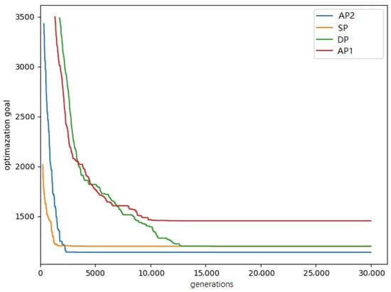
Figure 5. Comparation among the penalty method in the case.

By contrast, the SP and AP2 works better on both convergence time and the optimality of the scheduling. It is worth noting that the static method, as an old method, works quite well on our problem, although it still suffers from premature convergence, ended with the optimization goal to be 1201 h, while the exact optimal schedule objective is at most 1137 h appropriately. This is because its relatively simple way of calculating the penalty prevents the aforementioned degradation into a death penalty. However, its result is easily influenced by the coefficients $r_i$ of the penalty terms and it takes time to fine-tune the best coefficients of the penalty terms. Figure 6 shows the results of assigning coefficient $r_i$ with a same value. It can be seen that even if all $r_i$ are the same coefficients, the quality of the found optimal schedule objective still varies depending on the values of coefficient, let alone if $r_i$ are assigned different coefficients.

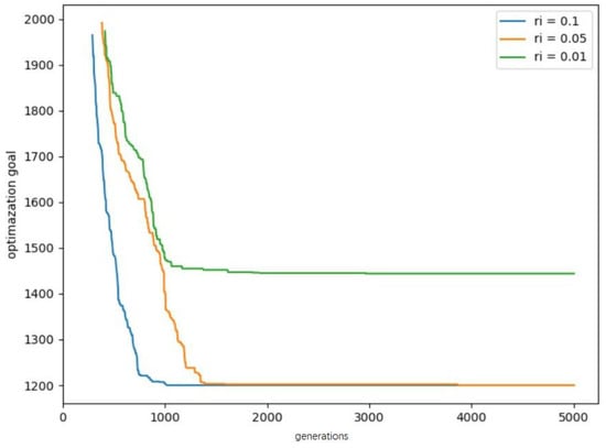
Figure 6. Result of assigning values to the penalty coefficient $r_i$.

5.3.2. Effect of Extinction Countdown

Figure 7 shows a population distribution situation during the evolution of GA after visualization using Principal Component Analysis (PCA) to reduce dimensions. It can be seen that individuals tend to cluster in some areas.

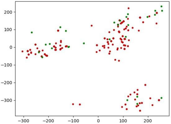
Figure 7. The distribution of GA’s population, when using static penalty at the 2000th generation. Each red point represents a feasible schedule solution and the green points represents the infeasible solutions.

Figure 8 shows the comparison of the results where there is and there is no extinction mechanism introduced. It can be seen that although the extinction mechanism cannot improve the convergence speed, it can obtain better schedules through iteration after convergence, and the value of $e$ makes difference. A too-small $e$ leads to a worse scheduling objective because the extinction happens before a better solution is generated.

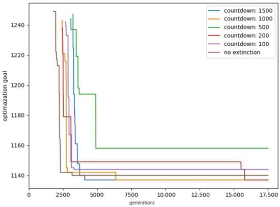
Figure 8. Comparation of the results where there is and there is no extinction mechanism introduced.

In any case, the above problems do not have an impact on the feasible optimal schedules that have already been produced. Figure 9 shows the fluctuations in inventory of several kinds of materials under the optimal scheduling. There is no case where the inventory is below the lower bound.

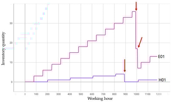
Figure 9. The fluctuations in inventory of two kinds of materials under the optimal scheduling. The red arrow indicates the material is used in a procedure.

Appendix A Table A1, Table A2, Table A3, Table A4 and Table A5 shows the other five cases of different set of production orders as input, and the result in Appendix A Figure A1 shows that our proposed algorithm can still calculate approximate optimal solutions in these cases. The results of the case studies shows that RCPSP-IR is capable to describe the scheduling problems in actual production scenarios, and our scheduling method based on GA is practical to solve RCPSP-IR. By conducting a series of comparative experiments of the hyper parameters and constraint handling methods, a production scheduling strategy with shorter production time objective can be obtained.

6. Discussion

The RCPSP-IR is proposed to formulate the scheduling problem of civil aircraft production. Despite the narrow feasible regions inherent in this combinatorial optimization problem, the obtained results demonstrate the feasibility and practicality of finding near-optimal solutions, forming an effective scheduling scheme for civil aircraft production.

In terms of convergence speed, AP2 outperforms DP and AP1 because AP2 can adaptively adjust the penalty terms, while DP and AP2 easily degrade to the death penalty situation. Moreover, from the point of view of the scheduling goal value that it finally converges to, AP2 shows a lower likelihood to fall into local optima for similar reasons. Additionally, compared with SP, AP2 also takes less effort to fine-tune parameters. By additionally importing extinction, local optimality can be further avoided. These efforts make the scheduler obtain faster scheduling schemes.

The purpose of our method is to schedule production activities in advance when order demands occur, providing a reference for the layout of production. As an approximate optimal scheduling scheme has been generated, it is possible to serve as guidance for production assembly. The results of this case study have already been used to guide the aircraft production assembly in COMAC.

7. Summary and Prospect

In this paper, we focus on providing a scheduling solution with the shortest production time for a station, leading to an improvement in station production efficiency. We propose a GA-based scheduling method for civil aircraft production, with considerations on material inventory replenishment. Based on the on-site research and investigation, we formulate the civil aircraft production scheduling problem as RCPSP-IR. To solve RCPSP-IR and achieve the minimum production time, GA with different constraint handling techniques is introduced. The results of the case study demonstrate that our proposed method can effectively obtain a nearly optimal scheduling strategy. This method has already been applied to guide practical production to improve production efficiency. For future work, we will further consider the interdependencies between multiple stations as well. The method can also be further improved by comprehensively considering other effects of production and supply chain links, such as service level, inventory levels, lead times, or costs.

References

- Guzman, E.; Andres, B.; Poler, R. Models and algorithms for production planning, scheduling and sequencing problems: A holistic framework and a systematic review. J. Ind. Inf. Integr. 2022, 27, 100287. [Google Scholar] [CrossRef]
- Lohmer, J.; Lasch, R. Production planning and scheduling in multi-factory production networks: A systematic literature review. Int. J. Prod. Res. 2021, 59, 2028–2054. [Google Scholar] [CrossRef]
- Beheshtinia, M.A.; Ghasemi, A. A multi-objective and integrated model for supply chain scheduling optimization in a multi-site manufacturing system. Eng. Optim. 2018, 50, 1415–1433. [Google Scholar] [CrossRef]
- Beheshtinia, M.A.; Ghasemi, A.; Farokhnia, M. Supply chain scheduling and routing in multi-site manufacturing system (case study: A drug manufacturing company). J. Model. Manag. 2018, 13, 27–49. [Google Scholar] [CrossRef]
- Maaoui, A.; Abdellatif, A.; Telmoudi, A.J.; Gattoufi, S.; Nabli, L. Multi-Site Manufacturing System Scheduling Using Petri Nets; IEEE: Piscataway, NJ, USA, 2018; pp. 469–474. [Google Scholar] [CrossRef]
- Chen, R.; Lu, J.; Zhang, H.; Xia, L. Research on scheduling problem of discrete manufacturing workshop for major equipment in complicated environment. Mater. Sci. Eng. 2019, 688, 055048. [Google Scholar] [CrossRef]
- Shan, S.; Hu, Z.; Liu, Z.; Shi, J.; Wang, L.; Bi, Z. An adaptive genetic algorithm for demand-driven and resource-constrained project scheduling in aircraft assembly. Inf. Technol. Manag. 2017, 18, 41–53. [Google Scholar] [CrossRef]
- Lovato, D.; Guillaume, R.; Thierry, C.; Battaia, O. Managing disruptions in aircraft assembly lines with staircase criteria. Int. J. Prod. Res. 2023, 61, 632–648. [Google Scholar] [CrossRef]
- Lu, Z.; Ren, Y.; Wang, L.; Zhu, H. A resource investment problem based on project splitting with time windows for aircraft moving assembly line. Comput. Ind. Eng. 2019, 135, 568–581. [Google Scholar] [CrossRef]
- Hartmann, S.; Briskorn, D. An updated survey of variants and extensions of the resource-constrained project scheduling problem. Eur. J. Oper. Res. 2022, 297, 1–14. [Google Scholar] [CrossRef]
- Ratajczak-Ropel, E.; Skakovski, A. Population-Based Approaches to the Resource-Constrained and Discrete-Continuous Scheduling; Springer: Berlin, Germany, 2018. [Google Scholar]
- Bartels, J.-H.; Gather, T.; Zimmermann, J. Dismantling of nuclear power plants at optimal NPV. Ann. Oper. Res. 2011, 186, 407–427. [Google Scholar] [CrossRef]
- Hartmann, S. Project scheduling with resource capacities and requests varying with time: A case study. Flex. Serv. Manuf. J. 2013, 25, 74–93. [Google Scholar] [CrossRef]
- Hartmann, S. Time-varying resource requirements and capacities. Handb. Proj. Manag. Sched. 2015, 1, 163–176. [Google Scholar]
- Hosseinian, A.H.; Baradaran, V.; Bashiri, M. Modeling of the time-dependent multi-skilled RCPSP considering learning effect: An evolutionary solution approach. J. Model. Manag. 2019, 14, 521–558. [Google Scholar] [CrossRef]
- Beşikci, U.; Bilge, Ü.; Ulusoy, G. Multi-mode resource constrained multi-project scheduling and resource portfolio problem. Eur. J. Oper. Res. 2015, 240, 22–31. [Google Scholar] [CrossRef]
- Habibi, F.; Barzinpour, F.; Sadjadi, S.J. A mathematical model for project scheduling and material ordering problem with sustainability considerations: A case study in Iran. Comput. Ind. Eng. 2019, 128, 690–710. [Google Scholar] [CrossRef]
- Patoghi, A.; Mousavi, S.M. A new approach for material ordering and multi-mode resource constraint project scheduling problem in a multi-site context under interval-valued fuzzy uncertainty. Technol. Forecast. Soc. Chang. 2021, 173, 121137. [Google Scholar] [CrossRef]
- Tabrizi, B.H. Integrated planning of project scheduling and material procurement considering the environmental impacts. Comput. Ind. Eng. 2018, 120, 103–115. [Google Scholar] [CrossRef]
- Zoraghi, N.; Shahsavar, A.; Niaki, S.T.A. A hybrid project scheduling and material ordering problem: Modeling and solution algorithms. Appl. Soft Comput. 2017, 58, 700–713. [Google Scholar] [CrossRef]
- Fu, F. Integrated scheduling and batch ordering for construction project. Appl. Math. Model. 2014, 38, 784–797. [Google Scholar] [CrossRef]
- Coello, C.A.C. Constraint-Handling Techniques Used with Evolutionary Algorithms; Association for Computing Machinery: New York, NY, USA, 2022; pp. 1310–1333. [Google Scholar]
- Tessema, B.; Yen, G.G. An adaptive penalty formulation for constrained evolutionary optimization. IEEE Trans. Syst. Man Cybern.-Part A Syst. Hum. 2009, 39, 565–578. [Google Scholar] [CrossRef]
- Dang, D.C.; Friedrich, T.; Kötzing, T.; Krejca, M.S.; Lehre, P.K.; Oliveto, P.S.; Sudholt, D.; Sutton, A.M. Escaping local optima using crossover with emergent diversity. IEEE Trans. Evol. Comput. 2017, 22, 484–497. [Google Scholar] [CrossRef]
Disclaimer/Publisher’s Note: The statements, opinions and data contained in all publications are solely those of the individual author(s) and contributor(s) and not of MDPI and/or the editor(s). MDPI and/or the editor(s) disclaim responsibility for any injury to people or property resulting from any ideas, methods, instructions or products referred to in the content. |
© 2023 by the authors. Licensee MDPI, Basel, Switzerland. This article is an open access article distributed under the terms and conditions of the Creative Commons Attribution (CC BY) license (https://creativecommons.org/licenses/by/4.0/).