Multiscale Model Reduction with Local Online Correction for Polymer Flooding Process in Heterogeneous Porous Media

Abstract

In this work, we consider a polymer flooding process in heterogeneous media. A system of equations for pressure, water saturation, and polymer concentration describes a mathematical model. For the construction of the fine grid approximation, we use a finite volume method with an explicit time approximation for the transports and implicit time approximation for the flow processes. We employ a loose coupling approach where we first perform an implicit pressure solve using a coarser time step. Subsequently, we execute the transport solution with a minor time step, taking into consideration the constraints imposed by the stability of the explicit approximation. We propose a coupled and splitted multiscale method with an online local correction step to construct a coarse grid approximation of the flow equation. We construct multiscale basis functions on the offline stage for a given heterogeneous field; then, we use it to define the projection/prolongation matrix and construct a coarse grid approximation. For an accurate approximation of the nonlinear pressure equation, we propose an online step with calculations of the local corrections based on the current residual. The splitted multiscale approach is presented to decoupled equations into two parts related to the first basis and all other basis functions. The presented technique provides an accurate solution for the nonlinear velocity field, leading to accurate, explicit calculations of the saturation and concentration equations. Numerical results are presented for two-dimensional model problems with different polymer injection regimes for two heterogeneity fields.

1. Introduction

Polymer flooding is an advanced technique used in the field of Enhanced Oil Recovery (EOR) to improve the recovery of viscous oil from reservoirs. It involves injecting a mixture of chemicals, including polymers and surfactants, to reduce the viscosity of the injected fluids during the flooding process. The flow behavior of polymeric solutions in porous media is recognized as a complex phenomenon, where the viscosity of a polymer solution plays a pivotal role in governing its flow characteristics [1,2,3]. The viscosity of a polymer solution is influenced by factors such as concentration, polymer structure, velocity, heterogeneity, and temperature [4,5,6]. The Flory–Huggins equation describes the viscosity of a polymeric solution at zero shear rates, which relates the viscosity to the concentration of the polymer [1,7,8,9]. The shear-thinning viscosity model accounts for the non-Newtonian behavior of polymer solutions, indicating that the viscosity decreases with increasing shear rate or flow velocity [10]. Polymer flooding has been the subject of extensive research over numerous years. However, its successful implementation remains a challenge primarily due to the highly heterogeneous nature of reservoir properties. These heterogeneities significantly impact the flow and transport processes, necessitating a specialized approach to constructing mathematical models and developing computational algorithms [8,11,12,13].

The reservoir properties and fluid behavior exhibit significant spatial and temporal variations at multiple scales. The heterogeneities can range from pore-scale variations to field-scale geological features. Capturing these fine-scale details in numerical simulations can be computationally prohibitive. Upscaling and multiscale methods are essential approaches that aim to bridge the gap between the fine-scale details of the reservoir and the practical computational requirements for reservoir-scale simulations. Various multiscale and homogenization methods have been extensively studied and developed in the field of reservoir simulations. Multiscale methods involve decomposing a system into multiple scales or levels of detail, each representing different physical phenomena or spatial resolutions. These methods consider the interactions and interdependencies between scales and provide a framework for capturing the effects of heterogeneity, nonlinearity, and other complex behaviors. Some commonly used multiscale methods include the Multiscale Finite Element Method [14,15], Mixed Multiscale Finite Element Method [16,17,18], Multiscale Finite Volume Method [19,20], Generalized Multiscale Finite Element Method [21,22,23,24], Constrain Energy Minimization method [25], and Non-Local Multi-Continua upscaling [26,27,28,29,29]. In [30], the authors considered the upscaling of parameters related to polymer flooding. The procedure involves three stages: (1) single-phase upscaling of the absolute permeability, (2) two-phase upscaling of relative permeabilities, and (3) upscaling of the parameters involved in polymer flooding. The upscaling–downscaling method of EOR simulation (polymer, surfactant, and thermal) was presented in [31]. In this algorithm, the pressure distribution is solved on the upscaled coarse grid, but the fine-scale heterogeneities are included in the computation of the saturations using a downscaled velocity. In [10], the extension of the multiscale restricted-smoothed basis method was presented for polymer flooding, including shear-thinning effects. Multiscale methods effectively reduce the computational complexity while preserving the system’s key characteristics that enable efficient computation by reducing the degrees of freedom in the simulation models.

This paper considers a polymer flooding process in heterogeneous porous media. A mathematical model is described by equations for the flow and transport (water saturation and polymer concentration). The convenient way to solve such problems includes the construction of a sufficiently fine grid that resolves heterogeneity on the grid level (fine grid). To approximate space variables, we use a finite volume approximation with explicit time approximation for the transports and implicit time approximation for the flow processes. Approximations on the fine grid lead to a large system of equations that are computationally expensive to solve. The main challenge is related to the pressure equation, which requires the solution of the large system of equations associated with the fine grid [10,31]. To reduce the cost associated with the pressure solution, we first apply a loose coupling approach. Loose coupling is closely related to the operator-splitting techniques and mutilate time stepping [32]. We apply a loose coupling algorithm to run a transport solve with a minor time step, which is restricted by the stability of the explicit approximation, and call an implicit pressure to solve with a coarser time step. The loosely coupled scheme is typical for multiphysics problems, where different time scales can characterize each sub-problems. In [33], the loose coupling algorithm is used for coupled fluid flow and geomechanical deformation simulation. In [34], the study of the partitioned solution procedure for thermomechanical coupling was presented, where a separate time integration scheme solves each sub-problem. The multirate iterative schemes for the poroelasticity problem are presented in [35], where the multirate iterative coupling scheme exploits the different time scales for the mechanics and flow problems by taking multiple finer time steps for flow within one coarse mechanics time step. In [32], the physics-based two-level operator splitting is used for two-phase flow problems with a multiscale solver for pressure solving. The two-level operator splitting is based on the split into the three sub-systems (elliptic in the pressure equation, hyperbolic, and parabolic in the saturation equation). The multiscale finite volume element method is applied for the elliptic and parabolic sub-systems.

In this work, we combine operator-splitting techniques with a multiscale approach for polymer flooding processes in heterogeneous porous media. Motivated by a loose coupling approach presented for a two-phase flow problem in [32], we extend it and investigate for the polymer flooding process, where for the pressure equation upscaling, we use a multiscale method with an online local correction process. The construction of reduced order model is based on the Generalized Multiscale Finite Element Method (GMsFEM). In GMsFEM, we construct multiscale basis functions on the offline stage for a given heterogeneous field; then, we use them to define the projection/prolongation matrix and construct a coarse grid approximation. However, for accurate solutions to nonlinear problems, the multiscale basis function should incorporate information about the current solution (saturation, concentration, and pressure). Such basis reconstruction is computationally expensive and leads to the regeneration of the projection matrix [36,37,38]. In this work, we propose a local online correction technique for the nonlinear pressure equation that arises in the simulation of the polymer flooding process. In local online correction, we use local residual information to correct the current multiscale solution in a set of non-overlapping local domains. Next, we construct the splitted multiscale approach based on the additive representation of the pressure matrix. We propose decoupling related to the multicontinuum types of problems for separating the primary continuum from others [39]. Furthermore, we can associate such splitting with separating the part related to the regular coarse grid approximation and the remaining part for the local spectral enrichment. The presented technique provides an accurate solution for the nonlinear velocity field, leading to accurate, explicit calculations of the saturation and concentration equations. We present numerical results for two-dimensional model problems with different polymer injection regimes for two hetergeneity fields. To test the presented coupled and splitted multiscale method, we investigate the influence of coarse grid size, the number of multiscale basis functions, the effect of the correction step, and loose coupling on the method’s accuracy.

The paper is organized as follows. In Section 2, we present a problem formulation with a basic mathematical model of the polymer flooding process and consider the construction of the discrete problem on the fine grid using a finite volume method, an explicit transport scheme and loose coupling with an implicit pressure solve. In Section 3, we construct a coupled and splitted multiscale method for the solution of the flow equation on the coarse grid, where we introduce offline and online stages with a local residual-based correction for nonlinear pressure problems. A numerical investigation is presented in Section 4 for two-dimensional model problems with different polymer injection regimes for two hetergeneity fields. Finally, the conclusion is presented.

2. Problem Formulation

This section starts with the mathematical model formulation for polymer flooding processes in porous media. Then, we define a fine grid approximation based on the finite volume method and discuss the construction of the time approximation with an explicit approximation for saturation and concentration equations.

2.1. Mathematical Model

The polymer flooding process in porous media can be mathematically represented by incorporating Darcy’s law and conservation laws for the water saturation and polymer concentration. In the case where the fluid and rock are incompressible and there are no gravitational or capillary forces, we have

$$\begin{array}{cc}\hfill \varphi \frac{\partial s}{\partial t}-\nabla ·({\lambda }_w(s,c)k\left(x\right)\nabla p)=f_w,& \hfill x\in \mathsf{\Omega },t>0,\hfill \\ \hfill \varphi \frac{\partial \left(sc\right)}{\partial t}-\nabla ·(c{\lambda }_w(s,c)k\left(x\right)\nabla p)=c{f}_w,& \hfill x\in \mathsf{\Omega },t>0,\hfill \\ \hfill -\nabla ·q=f_w+f_n,q=q_w+q_n,& \hfill x\in \mathsf{\Omega },\hfill \\ \hfill q_{\alpha }=-{\lambda }_{\alpha }(s,c)k\left(x\right)\nabla p,& \hfill x\in \mathsf{\Omega },\hfill \end{array}$$

(1)

where $s=s_w$ is the saturation of the wetting phase, c is the polymer concentration in the wetting phase, p is the pressure, $q_w$ and $q_n$ are the wetting and non-wetting phase fluxes, $f_{\alpha }$ is the source term of the $\alpha$-phase, $\varphi$ is the porosity, k is the heterogeneous permeability and

$${\lambda }_w(s,c)=k_{rw}\left(s\right)/{\mu }_w\left(c\right),{\lambda }_n\left(s\right)=k_{rn}\left(s\right)/{\mu }_n,\lambda ={\lambda }_w+{\lambda }_n,$$

(2)

here, ${\mu }_{\alpha }$ and $k_{r\alpha }$ are the viscosity and relative permeability for $\alpha$-phase ($\alpha =n,w$).

For the polymer flooding process, we use a linear law for wetting phase viscosity

$${\mu }_w\left(c\right)={\mu }_{wa}(1+\gamma c),$$

(3)

where ${\mu }_{wa}$ is the pure water viscosity and the coefficient $\gamma$ characterizes the particular polymer [4,7,8,9]. This model simplifies the zero shear rate Flory model with the neglected effect of the salinity [1,7,8,9]. We note that, in general, different types of relationships can be employed to characterize the viscosity of the wetting phase, and these variations do not significantly impact the overall algorithm proposed in this paper.

We supplement the mathematical model (1) with given initial conditions

$$s=s_0,c=c_0,p=p_0,t=0,$$

(4)

and zero flux boundary conditions.

2.2. Approximation Space on the Fine Grid

The conventional approach for constructing approximations is typically based on creating a grid that resolves heterogeneity at the grid level. This grid, which effectively resolves fine-scale details, will be referred to as the “fine grid” in this study. In this work, we consider a two-dimensional domain $\mathsf{\Omega }$.

Let ${\mathcal{T}}_h={\cup }_{i=1}^{N_f}{K}_i$ be the fine grid of the domain $\mathsf{\Omega }$, where $N_f$ is the number of cells. To construct a space approximation, we employ a finite volume method with a two-point flux approximation

$$q_{\alpha ,ij}\approx -{\lambda }_{\alpha }(s_{ij},c_{ij})W_{ij}(p_j-p_i),W_{ij}=k_{ij}\frac{|E_{ij}|}{d_{ij}},$$

(5)

where $k_{ij}$ is the harmonic average between $k_i$ and $k_j$ ($k_{ij}=2/(1/k_i+1/k_j)$), $|E_{ij}|$ is the length of face between cells $K_i$ and $K_j$, $d_{ij}$ is the distance between midpoints of cells $K_i$ and $K_j$ for $i=1,\dots ,N_f$, $N_f$ is the number of cells of the fine grid (Figure 1).

Figure 1. Heterogeneous permeability and fine grid (${\mathcal{T}}_h$).

For approximation of the ${\lambda }_w(s_{ij},c_{ij})$, we use an upwind scheme

$${\lambda }_w(s_{ij},c_{ij})=\left\{\begin{array}{cc}\hfill {\lambda }_w(s_i,c_i),\hfill & \hfill if T_{ij}(p_i-p_j)>0\hfill \\ \hfill {\lambda }_w(s_j,c_j),\hfill & \hfill \mathrm{otherwise},\hfill \end{array}\right..$$

Then, the system of Equation (1) can be written in the following semi-discrete way for each cell $K_i$

$$\begin{array}{cc}\hfill {\varphi }_i\frac{\partial s_i}{\partial t}\left|K_i\right|+& \hfill \sum _j{T}_{w,ij}(p_i-p_j)=f_{w,i}\left|K_i\right|,\hfill \\ \hfill {\varphi }_i\frac{\partial \left(s_i{c}_i\right)}{\partial t}\left|K_i\right|+& \hfill \sum _j{c}_{ij}{T}_{w,ij}(p_i-p_j)=c_i{f}_{w,i}\left|K_i\right|,\hfill \\ \hfill & \hfill \sum _j{T}_{ij}(p_i-p_j)=f_i\left|K_i\right|,\hfill \end{array}$$

(6)

where

$$T_{ij}=\lambda (s_{ij},c_{ij})W_{ij},T_{w,ij}={\lambda }_w(s_{ij},c_{ij})W_{ij},$$

and $\lambda (s_{ij},c_{ij})$ is the average between $\lambda (s_i,c_i)$ and $\lambda (s_j,c_j)$.

2.3. Approximation by Time and Loose Coupling

In this work, we use an explicit time approximation for the saturation and concentration problems, which leads to the standard IMPES scheme (implicit pressure, explicit saturation and concentration)

$$\begin{array}{cc}\hfill {\varphi }_i\frac{s_i^{n+1}-s_i^n}{\tau }\left|K_i\right|+& \hfill \sum _j{T}_{w,ij}^n(p_i^n-p_j^n)=f_{w,i}^n\left|K_i\right|,\hfill \\ \hfill {\varphi }_i\frac{s_i^{n+1}{c}_i^{n+1}-s_i^n{c}_i^n}{\tau }\left|K_i\right|+& \hfill \sum _j{c}_{ij}^n{T}_{w,ij}^n(p_i^n-p_j^n)=c_i^n{f}_{w,i}^n\left|K_i\right|,\hfill \\ \hfill & \hfill \sum _j{T}_{ij}^n(p_i^n-p_j^n)=f_i^n\left|K_i\right|,\hfill \end{array}$$

(7)

where n is the number of time steps and $\tau$ is the given time step size. We note that the time step size is chosen to satisfy a stability condition of the explicit scheme.

The pressure equation can be written in the following matrix form for $p={(p_1,\dots ,p_{N_f})}^T$

$$A^n{p}^n=F^n,$$

(8)

with

$$A^n=\left\{a_{ij}^n\right\},a_{ij}=\left\{\begin{array}{cc}\sum _j{T}_{ij}^n& i=j,\\ -T_{ij}^n& i\ne j\end{array}\right.,$$

where $F^n={(f_1^n,\dots .,f_{N_f}^n)}^T$ and $i=1,\dots ,N_f$.

We have the following algorithm for the fine grid problem:

• Initialize, saturation, concentration and pressure fields, using given initial conditions

  $$p^0=p_0,s^0=s_0,c^0=c_0.$$
• For each time iteration ($n=1,2,\dots ,N_t$):

  -

  Implicit pressure solve.

  Generate the fine scale matrix and right-hand side vector ($A^n$ and $F^n$) and solve the system of linear Equation (8) to find $p^n$.

  -

  Explicit transport solve.

  Update saturation and concentration using explicit formulas on the fine grid:

  $$\begin{array}{cc}\hfill s_i^{n+1}& \hfill =s_i^n+\frac{\tau }{{\varphi }_i}{f}_{w,i}^n-\frac{\tau }{{\varphi }_i\left|K_i\right|}\sum _j{T}_{w,ij}^n(p_i^n-p_j^n),\hfill \\ \hfill c_i^{n+1}& \hfill =\frac{1}{s_i^{n+1}}\left(s_i^n{c}_i^{n+1}+\frac{\tau }{{\varphi }_i}{c}_i^n{f}_{w,i}^n-\frac{\tau }{{\varphi }_i\left|K_i\right|}\sum _j{c}_{ij}^n{T}_{w,ij}^n(p_i^n-p_j^n)\right).\hfill \end{array}$$

  (9)

The main challenge in this problem is related to the pressure equation, which requires the solution of the large system of linear equations associated with the fine grid. To reduce the cost associated with the pressure solve, we first use a loose coupling approach to run an explicit transport solve for a set of time steps with fixed pressure (see Figure 2 for illustration).

Figure 2. Illustration of the loosely coupled time stepping.

Finally, we have the following loose coupled algorithm for the fine grid problem:

• Initialize, saturation, concentration and pressure fields, using given initial conditions, $p^0=p_0,s^0=s_0,c^0=c_0$.
• For each time iteration ($n=1,2,\dots ,N_t$):

  -

  If the remainder of dividing n by $n_p$ is equal to zero ($n_p$ is the given number). Then Implicit pressure solve.

  Generate the fine-scale matrix and right-hand side vector ($A^n$ and $F^n$) and solve the system of linear Equation (8) to find $p^n$.

  -

  Explicit transport solve.

  Update saturation and concentration using explicit formulas on the fine grid using (9).

A similar technique was considered in [32] with a multiscale approximation for a pressure field for a two-phase flow problem. In this work, we use a different multiscale method and investigate the influence of loose coupling on polymer flooding processes.

Next, we discuss constructing the reduced order model for pressure using the multiscale method.

3. Multiscale Model Reduction

We construct a coarse scale approximation for the pressure equation using the Generalized Multiscale Finite Element Method (GMsFEM). In GMsFEM, we construct a multiscale basis function to capture the behavior of the solution at a fine scale. The GMsFEM approach involves two stages: offline and online. In the offline stage, we define local domains (subdomains), construct multiscale basis functions by solving the local eigenvalue problems, and generate a projection matrix. In the online stage, we project fine-scale problems onto the multiscale space using a projection matrix and solve a reduced-order problem on the coarse grid. The solution obtained using GMsFEM provides an accurate representation of the multiscale behavior on the coarse scale grid and can be downscaled to the fine-scale resolution using a projection matrix. Finally, after calculating the pressure equation using the multiscale method, we calculate a saturation and concentration on the fine grid using explicit formulas.

The accuracy of the transport problem solution highly depends on the accuracy of the nonlinear velocity field that is calculated based on the current pressure distribution. To address this issue, we propose an additional online correction step that can significantly reduce the error of the multiscale method. The correction step is based on the local calculations in the subdomains using information about the current residuals.

3.1. Offline Stage

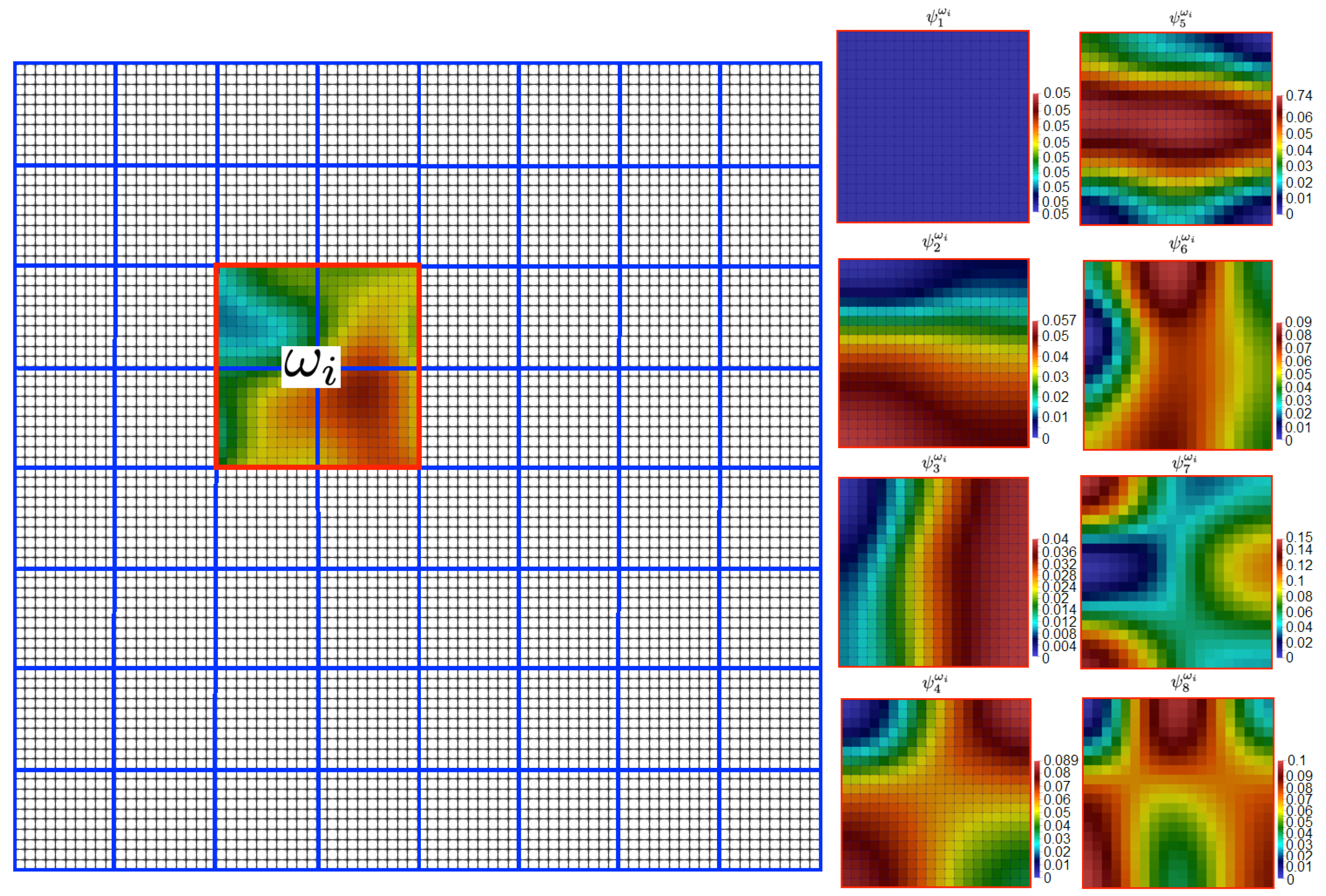
Let ${\mathcal{T}}_H$ be the coarse grid with cells $K_j$, and ${\omega }_i$ is the local domain related to the coarse grid node that is constructed as a combination of the several coarse cells that contains the corresponding coarse grid node (see Figure 3).

Figure 3. Coarse grid (blue lines, ${\mathcal{T}}_H$), fine grid (black lines), local domain (${\omega }_i$) and first eight eigenvalues (${\psi }_l^{{\omega }_i}$, $l=1,\dots ,8$.).

In order to construct multiscale basis functions on the offline stage for the nonlinear problem, we use a linear part of the pressure equation. In each local domain ${\omega }_i$, we solve the following eigenvalue problem

$$A^{{\omega }_i}{\psi }_l^{{\omega }_i}={\lambda }_l^{{\omega }_i}{S}^{{\omega }_i}{\psi }_l^{{\omega }_i},$$

(10)

with

$$A^{{\omega }_i}=\left\{a_{ij}\right\},a_{ij}=\left\{\begin{array}{cc}\sum _j{W}_{ij}& i=j,\\ -W_{ij}& i\ne j\end{array}\right.,S^{{\omega }_i}=\left\{s_{ij}\right\},s_{ij}=\left\{\begin{array}{cc}{k}_i\left|K_i\right|& i=j,\\ 0& i\ne j\end{array}\right.,i,j=1,\dots ,N_f^{{\omega }_i},$$

where $W_{ij}=k_{ij}\frac{|E_{ij}|}{d_{ij}}$ and $N_f^{{\omega }_i}$ is the number of coarse grid cells in the local domain ${\omega }_i$.

Next, we choose eigenvectors that correspond to the smallest $M_i$ eigenvalue ($0={\lambda }_1^{{\omega }_i}<{\lambda }_2^{{\omega }_i}<\dots <{\lambda }_{M_i}^{{\omega }_i}$) and create a projection matrix

$$R={\left[{\chi }^1{\psi }_1^{{\omega }_1},\dots ,{\chi }^1{\psi }_{M_1}^{{\omega }_1}\dots {\chi }^{N_c}{\psi }_1^{{\omega }_{N_c}},\dots ,{\chi }^{N_c}{\psi }_{M_{N_c}}^{{\omega }_{N_c}}\right]}^T.$$

(11)

where ${\chi }^i$ is the linear partition of unity functions, and $N_c$ is the number of the local domains (number of coarse grid nodes).

3.2. Online Stage

Once the projection matrix is constructed, the GMsFEM can be used to solve the problem on the coarse scale, taking advantage of the reduced dimension.

We use constructed multiscale basis functions to solve the pressure equation on the coarse grid. We use the projection matrix R to project the fine grid system to the coarse grid

$$A_H^n{p}_H^n=F_H^n,$$

(12)

with

$$A_H^n=R{A}^n{R}^T,F_H^n=R{F}^n.$$

(13)

After the solution of the reduced system, we reconstruct a fine grid solution

$$p_{ms}^n=R^T{p}_H^n.$$

(14)

Note that the size of the system is $N_c={\sum }_{i=1}^{N_v}{M}_i$, $M_i$ is the number of local multiscale basis functions in ${\omega }_i$ and $N_v$ is the number of coarse grid vertices. For the numerical investigation, we set to take the same number of basis functions in each local domain ($M_i=M$), and therefore, we have $N_c=M·N_v$. The convergence of the presented method depends on a number of local basis functions and coarse grid size.

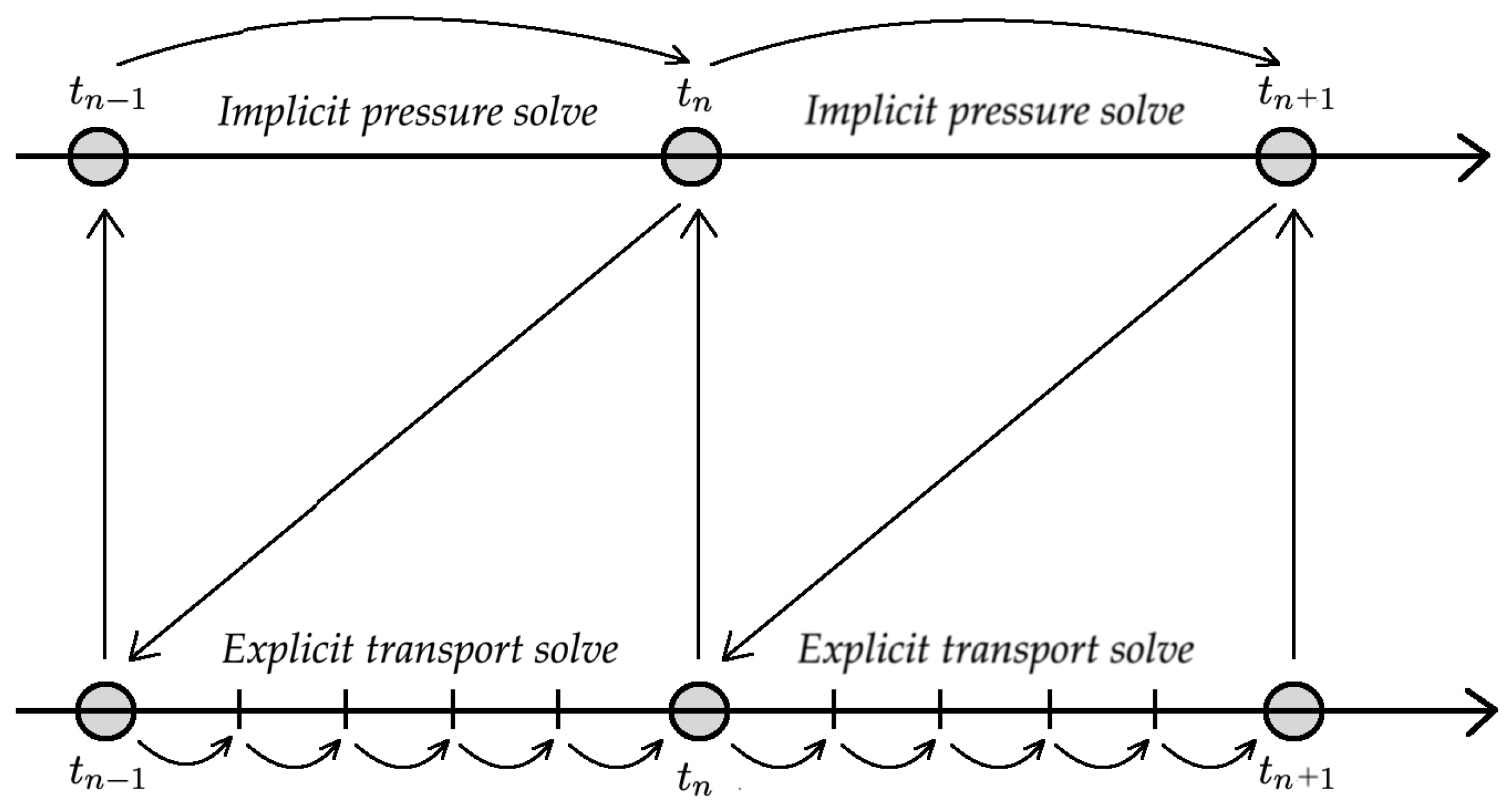
Then, on the online stage, we have the following algorithm for the transport and flow problem with loose coupling:

• Initialize saturation, concentration and pressure fields using initial conditions $p_h^0=p_0$, $s_h^0=s_0$, $c_h^0=c_0$ and project pressure onto the coarse grid $p_H^0=R{p}_h^0$.
• For each time iteration ($n=1,2,\dots ,N_t$):

  -

  If the remainder of dividing n by $n_p$ is equal to zero ($n_p$ is the given number). Then, Implicit pressure solve.

  Generate a fine scale matrix and right-hand side vector ($A^n$ and $F^n$), project the system onto coarse grid ($A_H^n=R{A}^n{R}^T$ and $F_H^n=R{F}^n$), solve the system of the linear Equation (12) to find $p_H^n$ and downscale the solution to fine grid $p_{ms}^n=R^T{p}_H^n$.

  -

  Explicit transport solve.

  Update saturation and concentration using explicit formulas on the fine grid:

  $$\begin{array}{cc}\hfill s_{ms,i}^{n+1}& \hfill =s_{ms,i}^n+\frac{\tau }{{\varphi }_i}{\tilde{f}}_{w,i}^n-\frac{\tau }{{\varphi }_i\left|K_i\right|}\sum _j{\tilde{T}}_{w,ij}^n(p_{ms,i}^n-p_{ms,j}^n),\hfill \\ \hfill c_{ms,i}^{n+1}& \hfill =\frac{1}{s_{ms,i}^{n+1}}\left(s_{ms,i}^n{c}_{ms,i}^{n+1}+\frac{\tau }{{\varphi }_i}{c}_{ms,i}^n{\tilde{f}}_{w,i}^n-\frac{\tau }{{\varphi }_i\left|K_i\right|}\sum _j{c}_{ms,ij}^n{\tilde{T}}_{w,ij}^n(p_{ms,i}^n-p_{ms,j}^n)\right),\hfill \end{array}$$

  (15)

  where ${\tilde{f}}_{w,i}$ and ${\tilde{T}}_{w,ij}^n$ are calculated using a multiscale solution $s_{ms,ij}^n,c_{ms,ij}^n$ and $p_{ms,ij}^n$.

The accuracy of the transport problem solution highly depends on the accuracy of the nonlinear velocity field that is calculated based on the current pressure distribution. To address this issue, we propose an additional online correction step that can significantly reduce the error of the multiscale method.

3.3. Online Residual-Based Local Correction

The correction step is based on the local calculations in the subdomains using information about the current residuals. After the solution of the pressure Equation (12), in each local domain, we find a local residual and solve the following local problem in ${\omega }_i$

$$A^{{\omega }_i}{\varphi }^{{\omega }_i}=r^{{\omega }_i},$$

(16)

with

$$A^{{\omega }_i}=\left\{a_{ij}\right\},a_{ij}=\left\{\begin{array}{cc}\sum _j{T}_{ij}^n& i=j,\\ -T_{ij}^n& i\ne j\end{array}\right.,$$

(17)

$$r^{{\omega }_i}=\left\{r_i^{{\omega }_i}\right\},r_i^{{\omega }_i}=f_{ms,i}^n-\sum _j{T}_{ms,ij}^n(p_{ms,i}^n-p_{ms,j}^n),$$

(18)

with zero Dirichlet boundary conditions except for the global boundary, where we set a zero Newman boundary condition.

We construct a local correction ${\varphi }^{{\omega }^i}$ in a non-overlapping set of local domains ${\omega }_i\in B^k$, where for the quadratic coarse cells, we have for sets of local domains (see the first row in Figure 4). The correction function in the kth set of subdomains is used to update the solution

$$p_{ms}^{n,k}=p_{ms}^{n,k-1}+\sum _{{\omega }_i\in B^k}{\varphi }^{{\omega }_i,k},$$

(19)

where $p_{ms}^{n,0}$ is the solution of Problem (12) and

$$A^{{\omega }_i}{\varphi }^{{\omega }_i,k}=r^{{\omega }_i,k-1},$$

(20)

with

$$r^{{\omega }_i,k-1}=\left\{r_i\right\},r_i=f_{ms,i}^{n,k}-\sum _j{T}_{ms,ij}^n(p_{ms,i}^{n,k-1}-p_{ms,j}^{n,k-1}).$$

(21)

Figure 4. Illustration of online residual-based local correction using non-overlapping subdomains ${\omega }_i\in B^k$ ($k=1,2,3,4$ from left to right) for $8\times 8$ coarse grid.

We have the following algorithm:

• Initialize saturation, concentration, and pressure fields using initial conditions $p_h^0=p_0$, $s_h^0=s_0$, $c_h^0=c_0$ and project pressure onto the coarse grid $p_H^0=R{p}_h^0$.
• For each time iteration ($n=1,2,\dots ,N_t$):

  -

  If the remainder of dividing n by $n_p$ is equal to zero ($n_p$ is the given number). Then, Implicit pressure solve.

  *

  Generate fine scale matrix and right-hand side vector ($A^n$ and $F^n$), project system onto coarse grid ($A_H^n=R{A}^n{R}^T$ and $F_H^n=R{F}^n$), solve system of linear Equation (12) to find $p_H^n$ and downscale the solution to fine grid $p_{ms}^n=R^T{p}_H^n$.

  *

  For each set of non-oversampling local domains $B^k$, $k=1,2,3,4$ iteratively calculate local corrections in ${\omega }_i\in B^k$ and update current solution using (19) and (20).

  -

  Explicit transport solve.

  Update saturation and concentration using explicit Formula (15) with $p_{ms}^n=p_{ms}^{n,4}$.

The proposed online correction, similar to the multiscale basis functions calculations, is based on the local calculations in a non-overlapping set of local domains ${\omega }_i$. For the case of quadratic cells, we have four sets of non-overlapping subdomains. Moreover, this additional step does not affect the size of the coarse scale system.

3.4. Multiscale Splitting Approach

A regular multiscale method (GMsFEM), considered above, leads to the solution of the coupled system of equations related to a number of basis functions with size $N_c={\sum }_i{M}_i$. Next, instead of the solution of the coupled system of linear equations on each time step, we use an additive representation of the matrix to construct an uncoupled scheme for the pressure equation. In this work, we propose a decoupling related to the multicontinuum types of problems to separate the primary continuum from others [39]. Furthermore, we know that the first eigenvalue is the constant, and therefore, the resulting first basis is the regular bi-linear partition of the unity function. Therefore, we can associate such a type of splitting with the separation of the part related to the regular coarse grid approximation and remain a part with the local spectral enrichment. This approach is highly connected with our recent work [39], where we proposed a novel splitting algorithm for the flow in fractured porous media.

Let $R={[R_1,R_2]}^T$, where $R^1$ is constructed based on the first basis function for each local domain, and $R^2$ contains the remaining basis functions, i.e.,

$$\begin{array}{cc}\hfill & \hfill R_1={\left[{\chi }^1{\psi }_1^{{\omega }_1},\dots {\chi }^{N_c}{\psi }_1^{{\omega }_{N_c}}\right]}^T,\hfill \\ \hfill & \hfill R_2={\left[{\chi }^1{\psi }_2^{{\omega }_1},\dots ,{\chi }^{N_c}{\psi }_{M_1}^{{\omega }_1}\dots {\chi }^{N_c}{\psi }_2^{{\omega }_{N_c}},\dots ,{\chi }^{N_c}{\psi }_{M_{N_c}}^{{\omega }_{N_c}}\right]}^T.\hfill \end{array}$$

(22)

Then, instead of (12), we can use the following form of the coarse-scale system of pressure

$$\begin{array}{c}\hfill A_{H,11}^n{p}_H^{n,1}+A_{H,12}^n{p}_H^{n,2}=F_H^{n,1},\\ \hfill A_{H,21}^n{p}_H^{n,1}+A_{H,22}^n{p}_H^{n,2}=F_H^{n,2},\end{array}$$

(23)

where

$$A_H^n=\left(\begin{array}{cc}{A}_{H,11}^n& A_{H,12}^n\\ A_{H,21}^n& A_{H,22}^n\end{array}\right)=\left(\begin{array}{cc}{R}_1{A}^n{R}_1^T& R_1{A}^n{R}_2^T\\ R_2{A}^n{R}_1^T& R_2{A}^n{R}_2^T\end{array}\right),$$

(24)

$$F_H^n=\left(\begin{array}{c}{F}_{H,1}^n\\ F_{H,2}^n\end{array}\right)=\left(\begin{array}{c}{R}_1{F}^n\\ R_2{F}^n\end{array}\right),p_H^n=\left(\begin{array}{c}{p}_{H,1}^n\\ p_{H,2}^n\end{array}\right)=\left(\begin{array}{c}{R}_1{p}_h^n\\ R_2{p}_h^n\end{array}\right).$$

(25)

The construction of the multiscale splitting approach is based on an additive representation of the pressure operator

$$A_H^n=A_H^{n,1}+A_H^{n,2},$$

(26)

with

$$A_H^{n,1}=\left(\begin{array}{cc}{A}_{H,11}^n& 0\\ A_{H,21}^n& A_{H,22}^n\end{array}\right),A_H^{n,2}=A_H^n-A_H^{n,1},$$

(27)

Here, we approximate the coupling term in the first equation using the previous time layer and obtain the following multiscale splitting scheme

$$A_H^{n,1}{p}_H^n+A_H^{n,2}{p}_H^{n-1}=F_H^n.$$

(28)

where $p_H^{n-1}$ is the known solution from the previous time layer.

Such a representation leads to the independent calculations of the problems related to the first basis, and all remain basis functions

$$\begin{array}{c}\hfill A_{H,11}^n{p}_H^{n,1}+A_{H,12}^n{p}_H^{n-1,2}=F_H^{n,1},\\ \hfill A_{H,21}^n{p}_H^{n,1}+A_{H,22}^n{p}_H^{n,2}=F_H^{n,2},\end{array}$$

(29)

This system is decoupled, and allows us to first calculate solution $p_H^{n,1}$ and then find $p_H^{n,2}$ using $p_H^{n,1}$.

Finally, we have the following algorithm:

• Initialize saturation, concentration, and pressure fields using initial conditions $p_h^0=p_0$, $s_h^0=s_0$, $c_h^0=c_0$ and project pressure onto the coarse grid $p_H^0=R{p}_h^0$.
• For each time iteration ($n=1,2,\dots ,N_t$):

  -

  If the remainder of dividing n by $n_p$ is equal to zero ($n_p$ is the given number). Then, Implicit pressure solve.

  *

  Generate fine scale matrix and right-hand side vector ($A^n$ and $F^n$), and project system onto coarse grid

  $$A_H^n=\left(\begin{array}{cc}{A}_{H,11}^n& A_{H,12}^n\\ A_{H,21}^n& A_{H,22}^n\end{array}\right)=\left(\begin{array}{cc}{R}_1{A}^n{R}_1^T& R_1{A}^n{R}_2^T\\ R_2{A}^n{R}_1^T& R_2{A}^n{R}_2^T\end{array}\right),F_H^n=\left(\begin{array}{c}{F}_{H,1}^n\\ F_{H,2}^n\end{array}\right)=\left(\begin{array}{c}{R}_1{F}^n\\ R_2{F}^n\end{array}\right).$$

  Solve system of linear equations to find $p_H^{n,1}$

  $$A_{H,11}^n{p}_H^{n,1}=F_H^{n,1}-A_{H,12}^n{p}_H^{n-1,2},$$

  Solve system of linear equations to find $p_H^{n,2}$

  $$A_{H,22}^n{p}_H^{n,2}=F_H^{n,2}-A_{H,21}^n{p}_H^{n,1},$$

  Downscale the solution to fine grid $p_{ms}^n=R^T{p}_H^n$ with $p_H^n={[p_H^{n,1},p_H^{n,2}]}^T$.

  *

  For each set of non-oversampling local domains $B^k$, $k=1,2,3,4$ iteratively calculate local corrections in ${\omega }_i\in B^k$ and update current solution using (19) and (20).

  -

  Explicit transport solve.

  Update saturation and concentration using explicit Formula (15) with $p_{ms}^n=p_{ms}^{n,4}$.

4. Numerical Results

We consider the solution of the flow and transport in heterogeneous porous media ($\mathsf{\Omega }=[0,1]\times [0,1]$). We set source terms $f^{\pm }=\pm q$, $q={10}^3$ on left and right boundaries. For the nonlinear coefficient, we use $k_w=s^2$ and $k_n={(1-s)}^2$, $\varphi =1$, $m{u}_w=1$, ${\mu }_{wa}=5$ and $\gamma =4$ [4,7,9]. We consider two permeability fields for the numerical investigation. Both permeabilities are generated using the Karhunen–Loéve expansion [40,41]. The Gaussian covariance matrix is used with with correlation lengths $l_x=0.2$, $l_y=0.2$ for Heterogeneity-1 and $l_x=0.4$, $l_y=0.1$ for Heterogeneity-2. Figure 5 shows a permeability $k\left(x\right)$ for Heterogeneity-1 and Heterogeneity-2. The fine grid is $80\times 80$, and the coarse grid is $4\times 4$, $8\times 8$ and $16\times 16$ (see Figure 5).

Figure 5. Heterogeneous permeability (Heterogeneity-1 and Heterogeneity-2) and coarse grids ($4\times 4$, $8\times 8$, and $16\times 16$ (green color) with fine grid (blue color)).

We consider four test problems with different polymer injection options:

• Test 1. Pure water injection: $c_{inj}\left(t_m\right)=0$ and $s_{inj}\left(t_m\right)=1$ for $m=0,1,2\dots$.
• Test 2. Injection of polymer in first 100 time steps: $c_{inj}\left(t_m\right)=1$, $s_{inj}\left(t_m\right)=1$ for $m<100$ and $c_{inj}\left(t_m\right)=0$, $s_{inj}\left(t_m\right)=1$ for $m\ge 100$.
• Test 3. Injection of polymer in first 200 time steps: $c_{inj}\left(t_m\right)=1$, $s_{inj}\left(t_m\right)=1$ for $m<200$ and $c_{inj}\left(t_m\right)=0$, $s_{inj}\left(t_m\right)=1$ for $m\ge 200$.
• Test 4. Injection of polymer: $c_{inj}\left(t_m\right)=1$, $s_{inj}\left(t_m\right)=1$ for $m=0,1,2\dots$.

We set initial conditions $s_0=0.2$, $c_0=0$ and simulate 500 time steps with $\tau =0.8\times {10}^{-4}$ for Heterogeneity-1 and $\tau =0.4\times {10}^{-4}$ for Heterogeneity-2.

In Figure 6 and Figure 7, we depict the reference (fine grid) solution for Heterogeneity-1 and Heterogeneity-2, respectively. The simulation results are presented for Test 1, 2, 3 and 4 (from top to bottom). The pressure, saturation and concentration, $p^{500}$, $s^{100}$, $s^{300}$, $s^{500}$, $c^{100}$, $c^{300}$ and $c^{500}$ are depicted from left to right. We observe a significant influence of the heterogeneity field on the solution, where both probabilities are highly heterogeneous, and Heterogeneity-2 exhibits channelized features. Moreover, in Figure 6 and Figure 7, we observe a comparison between different polymer injection options in Test 1, 2, 3 and 4.

Figure 6. Heterogeneity-1. Fine grid solution for Test 1, 2, 3 and 4.

Figure 7. Heterogeneity-2. Fine grid solution for Test 1, 2, 3 and 4.

To compare the accuracy of the presented multiscale method and splitting techniques, we use the relative $L_2$ error in percentage for the saturation, concentration and pressure fields. Additionally, we calculate errors for the total and wetting phase velocity fields. We use the corresponding fine-grid solution for each test problem as a reference solution. The errors are calculated using the following formulas on the fine grid:

$$e_p^n=\frac{\left|\right|p^n-p_{ms}^n{\left|\right|}_{L_2}}{\left|\right|p^n{\left|\right|}_{L_2}}\times 100\%,e_s^n=\frac{\left|\right|s^n-s_{ms}^n{\left|\right|}_{L_2}}{\left|\right|s^n{\left|\right|}_{L_2}}\times 100\%,e_c^n=\frac{\left|\right|c^n-c_{ms}^n{\left|\right|}_{L_2}}{\left|\right|c^n{\left|\right|}_{L_2}}\times 100\%,$$

using the $L_2$ norm

$${\left|\right|v\left|\right|}_{L_2}^2=\sum _{i=1}^{N_f}{v}_i^2.$$

Here, n is the time layer; $p^n$, $s^n$ and $c^n$ are the reference (fine grid) solution; $p_{ms}^n$, $s_{ms}^n$ and $c_{ms}^n$ are the solution using the multiscale method.

Additionally, we calculate errors for the wetting phase velocity and total velocity

$$e_{u_w}^n=\frac{\left|\right|u_w^n-u_{w,ms}^n{\left|\right|}_{L_2}}{\left|\right|u_w^n{\left|\right|}_{L_2}}\times 100\%,e_u^n=\frac{\left|\right|u^n-u_{ms}^n{\left|\right|}_{L_2}}{\left|\right|u^n{\left|\right|}_{L_2}}\times 100\%,$$

where $u_w^n$ and $u^n$ are the wetting and total velocities calculated based on the fine grid solution (reference solution); $u_{w,ms}^n$ and $u_{ms}^n$ are the multiscale solutions based on wetting and total velocities. The accuracy of the velocity field directly affects the explicitly calculated saturation and concentration field errors.

Next, we present the numerical study results for the splitted multiscale approach. We start with the traditional coupled multiscale approach, where pressure is solved using the generalized multiscale finite element method with and without an online correction. We vary a number of multiscale basis functions to investigate the influence on the method’s accuracy. Then, we present results for the splitted multiscale approach, where we decouple part of the equation related to the first basis function or primary continuum [39,42]. Finally, we combine the multiscale splitting approach with the loose coupling approach for transport and pressure equations.

4.1. Multiscale Method with Online Correction

We consider the traditional coupled multiscale approach, where pressure is solved using a generalized multiscale finite element method with and without online correction. We vary a number of multiscale basis functions to investigate the influence on the method’s accuracy. We start with Heterogeneity-1.

In Table 1, Table 2 and Table 3, we present relative errors for three coarse grids $4\times 4$, $8\times 8$ and $16\times 16$ for Heterogeneity-1. We start by discussing the multiscale approximation results without a local correction step. We observe good results for all test cases with a sufficient number of multiscale basis functions for the pressure that can provide a good approximations of fluxes. For example, when we take 16 multiscale basis functions, we have less than one percent of error for the pressure field on the $4\times 4$ coarse grid in all tests (see Table 1). However, the wetting phase velocity error is significant (6.7%, 8.4%, 9.3%, and 6.4% for Test 1, 2, 3 and 4, which directly affects the saturation and concentration. For example, we have 5.4% and 6.5% of errors for saturation and concentration in Test 2. In Test 4, we observe more minor errors with 3.7% and 1.5% for saturation and concentration. On the $8\times 8$ coarse grid compared with the $4\times 4$ grid, we observe better results for the wetting phase velocity. For 16 multiscale basis functions, we obtain nearly one percent of the velocity error, which directly affects the saturation and concentration errors. We provide results with 0.9–1.3% for saturation and 0.2–1.5% for concentration (Table 2). For the $16\times 16$ coarse grid, we obtain less than one percent of errors for velocity, saturation, and concentration for all test cases using 12 and 16 basis functions (Table 3). Furthermore, we obtain a more significant error in Test 2and the slightest error in Test 4in all coarse grids.

Table 1. Heterogeneity-1. Relative errors at final time. Coarse mesh $4\times 4$.

	${\mathit{e}}_{\mathit{p}}$ (%)	${\mathit{e}}_{{\mathit{u}}_{\mathit{w}}}$ (%)	${\mathit{e}}_{\mathit{u}}$ (%)	${\mathit{e}}_{\mathit{s}}$ (%)	${\mathit{e}}_{\mathit{c}}$ (%)	${\mathit{e}}_{\mathit{p}}$ (%)	${\mathit{e}}_{{\mathit{u}}_{\mathit{w}}}$ (%)	${\mathit{e}}_{\mathit{u}}$ (%)	${\mathit{e}}_{\mathit{s}}$ (%)	${\mathit{e}}_{\mathit{c}}$ (%)
Test 1
1	13.109	53.602	40.242	38.159	-	4.656	16.506	12.423	9.203	-
2	8.527	47.568	36.327	29.041	-	3.236	9.389	7.454	5.594	-
4	4.272	28.271	22.364	16.899	-	1.162	3.612	2.796	1.924	-
8	2.008	19.640	15.190	12.081	-	0.247	0.984	0.744	0.519	-
12	1.382	20.212	15.221	10.216	-	0.050	0.245	0.185	0.118	-
16	0.431	6.731	5.123	3.668	-	0.062	0.240	0.183	0.124	-
Test 2
1	28.402	66.114	46.950	46.377	98.920	4.673	19.168	13.967	10.987	25.881
2	29.824	57.313	42.518	37.557	75.903	1.693	9.518	7.830	4.779	11.946
4	15.097	33.321	24.445	26.593	54.558	0.928	3.798	3.204	2.593	4.506
8	10.098	24.065	19.532	15.986	34.170	0.300	1.265	1.046	0.880	1.396
12	1.900	21.651	17.337	11.193	16.740	0.081	0.312	0.265	0.194	0.374
16	0.706	8.438	6.806	5.479	6.599	0.075	0.278	0.233	0.170	0.291
Test 3
1	20.887	67.125	48.138	47.346	81.318	2.854	19.145	13.709	11.665	26.816
2	24.285	60.581	43.811	39.228	64.401	1.231	9.699	7.854	4.320	10.816
4	14.952	34.354	25.698	26.539	39.849	0.474	4.242	3.510	2.006	4.006
8	9.012	23.394	17.943	16.043	19.783	0.142	1.201	0.970	0.644	1.132
12	2.710	19.450	15.358	9.628	9.472	0.037	0.282	0.224	0.148	0.253
16	1.215	9.367	7.623	5.350	4.905	0.030	0.233	0.186	0.125	0.200
Test 4
1	14.478	52.969	35.938	38.358	42.691	5.280	9.978	5.971	5.835	6.114
2	8.852	46.533	29.130	31.767	30.398	2.848	5.558	3.746	3.151	2.076
4	5.848	27.592	17.430	19.771	14.384	1.051	2.427	1.606	1.360	0.694
8	2.123	16.723	11.072	10.801	5.551	0.229	0.676	0.419	0.390	0.213
12	0.913	14.237	8.748	7.652	2.962	0.036	0.234	0.129	0.130	0.085
16	0.567	6.450	4.189	3.781	1.561	0.052	0.207	0.124	0.114	0.060

Table 2. Heterogeneity-1. Relative errors at final time. Coarse mesh $8\times 8$.

	${\mathit{e}}_{\mathit{p}}$ (%)	${\mathit{e}}_{{\mathit{u}}_{\mathit{w}}}$ (%)	${\mathit{e}}_{\mathit{u}}$ (%)	${\mathit{e}}_{\mathit{s}}$ (%)	${\mathit{e}}_{\mathit{c}}$ (%)	${\mathit{e}}_{\mathit{p}}$ (%)	${\mathit{e}}_{{\mathit{u}}_{\mathit{w}}}$ (%)	${\mathit{e}}_{\mathit{u}}$ (%)	${\mathit{e}}_{\mathit{s}}$ (%)	${\mathit{e}}_{\mathit{c}}$ (%)
Test 1
1	8.159	49.825	38.005	30.380	-	6.140	9.177	7.575	8.756	-
2	4.001	34.635	26.820	20.491	-	1.381	2.106	1.680	2.075	-
4	1.627	15.875	12.414	10.666	-	0.707	1.024	0.826	0.922	-
8	0.614	9.661	7.461	6.000	-	0.184	0.353	0.275	0.298	-
12	0.099	1.903	1.674	1.300	-	0.010	0.047	0.035	0.029	-
16	0.068	1.631	1.240	1.009	-	0.004	0.020	0.015	0.013	-
Test 2
1	30.648	57.487	39.132	39.987	80.954	3.218	16.619	13.803	9.749	27.697
2	13.984	41.214	32.014	25.225	47.403	1.398	3.426	2.822	3.318	7.066
4	3.581	18.364	15.131	12.398	21.862	0.588	1.334	1.097	1.233	2.584
8	0.756	11.339	9.565	6.336	7.943	0.147	0.378	0.317	0.344	0.722
12	0.172	2.434	2.168	1.834	2.259	0.014	0.082	0.069	0.046	0.083
16	0.100	1.728	1.411	1.252	1.516	0.006	0.036	0.030	0.019	0.035
Test 3
1	23.910	59.049	39.265	40.345	59.317	1.940	15.230	12.078	8.658	20.310
2	14.129	37.456	27.962	24.329	31.922	0.615	3.700	3.000	2.423	4.779
4	5.460	21.880	17.404	13.326	14.260	0.310	1.704	1.386	1.057	2.088
8	1.866	10.453	8.675	6.325	6.814	0.088	0.420	0.327	0.319	0.600
12	0.218	3.380	2.820	1.890	1.860	0.008	0.047	0.035	0.032	0.057
16	0.069	2.478	1.995	1.327	1.281	0.004	0.025	0.019	0.014	0.023
Test 4
1	7.747	45.956	24.910	30.230	26.341	6.316	7.457	5.004	5.337	5.465
2	4.445	27.459	16.847	18.224	11.225	1.754	2.167	1.471	1.890	1.274
4	1.963	16.082	10.149	11.325	6.178	0.884	1.144	0.770	0.893	0.547
8	0.905	8.847	5.937	5.964	2.223	0.248	0.377	0.248	0.295	0.161
12	0.098	1.897	1.470	1.323	0.320	0.016	0.040	0.026	0.027	0.013
16	0.051	1.577	0.986	0.951	0.228	0.007	0.016	0.010	0.011	0.006

Table 3. Heterogeneity-1. Relative errors at final time. Coarse mesh $16\times 16$.

	${\mathit{e}}_{\mathit{p}}$ (%)	${\mathit{e}}_{{\mathit{u}}_{\mathit{w}}}$ (%)	${\mathit{e}}_{\mathit{u}}$ (%)	${\mathit{e}}_{\mathit{s}}$ (%)	${\mathit{e}}_{\mathit{c}}$ (%)	${\mathit{e}}_{\mathit{p}}$ (%)	${\mathit{e}}_{{\mathit{u}}_{\mathit{w}}}$ (%)	${\mathit{e}}_{\mathit{u}}$ (%)	${\mathit{e}}_{\mathit{s}}$ (%)	${\mathit{e}}_{\mathit{c}}$ (%)
Test 1
1	3.195	33.424	25.467	19.233	-	2.085	2.680	2.142	2.277	-
2	1.096	21.183	16.400	12.278	-	0.512	0.853	0.653	0.704	-
4	0.523	10.060	7.948	5.913	-	0.235	0.500	0.384	0.346	-
8	0.222	5.523	4.293	3.205	-	0.060	0.149	0.116	0.090	-
12	0.024	1.100	0.868	0.595	-	0.004	0.022	0.016	0.012	-
16	0.012	0.843	0.610	0.355	-	0.001	0.007	0.006	0.004	-
Test 2
1	14.993	35.648	26.577	25.360	44.449	1.848	3.941	3.196	3.499	9.187
2	5.526	23.660	19.016	13.679	22.629	0.531	1.086	0.868	1.041	2.333
4	0.625	11.491	9.582	6.639	8.416	0.248	0.609	0.494	0.470	0.987
8	0.272	6.611	5.538	3.424	4.546	0.070	0.180	0.147	0.125	0.289
12	0.038	1.196	0.997	0.636	0.562	0.005	0.021	0.018	0.014	0.023
16	0.016	0.978	0.752	0.406	0.267	0.001	0.009	0.007	0.005	0.006
Test 3
1	14.025	35.884	25.831	26.058	33.289	0.903	4.806	3.908	2.965	5.788
2	6.630	22.824	17.767	14.249	19.666	0.262	1.324	1.066	0.934	1.631
4	1.248	11.978	9.837	6.352	7.223	0.149	0.702	0.574	0.421	0.691
8	0.301	7.141	5.852	3.361	3.516	0.041	0.173	0.143	0.100	0.176
12	0.033	1.241	1.038	0.648	0.480	0.003	0.022	0.019	0.012	0.015
16	0.015	0.646	0.498	0.372	0.239	0.001	0.007	0.005	0.004	0.004
Test 4
1	4.207	29.678	16.486	19.193	11.964	2.504	2.360	1.600	1.929	1.602
2	1.539	18.572	11.605	10.935	5.152	0.657	0.782	0.510	0.634	0.445
4	0.804	9.710	6.374	6.250	2.547	0.324	0.423	0.264	0.326	0.216
8	0.399	6.013	3.835	3.530	1.188	0.078	0.132	0.087	0.085	0.054
12	0.019	1.143	0.717	0.631	0.123	0.006	0.019	0.012	0.011	0.005
16	0.008	0.787	0.448	0.350	0.075	0.001	0.006	0.004	0.004	0.002

Next, we consider results with the local online correction and discuss the effect of the correction on the errors of the velocity field and the corresponding saturation and concentration errors. From the presented results in Table 1, Table 2 and Table 3, we observe a considerable error reduction after the application of the presented local correction step using residual information. In Table 1, we reduce the saturation error from 16% to 1.9% using the online correction step for the case with four multiscale basis functions in Test 1. In Test 4, we have 27%, 19%, and 14% of errors for the wetting phase velocity, saturation, and concentration using four basis functions. For the algorithm with a local online correction, we reduce errors to 2.4%, 1.3%, and 0.6% for wetting phase velocity, saturation, and concentration. In Test 2 and 3, we obtain excellent results for the online correction for the multiscale solution with eight basis functions, where we have 0.8 and 1.3% of error for saturation and concentration in Test 2, and 0.6 and 1.1% of error for saturation and concentration in Test 2. However, we obtain an excellent error reduction only when we use a sufficient number of preconstructed basis functions. On the finer coarse grid ($8\times 8$ in Table 2 and $16\times 16$ in Table 3), we observe good results for all test cases using four multiscale basis functions and two multiscale basis functions for $8\times 8$ and $16\times 16$ grids, respectively.

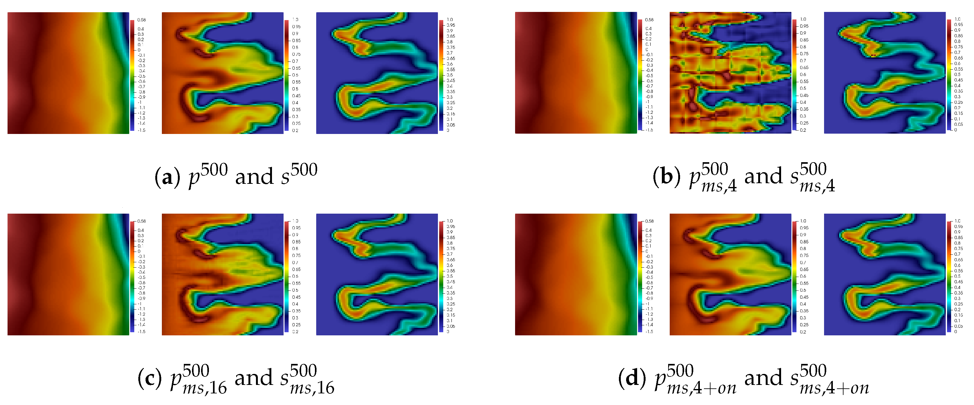
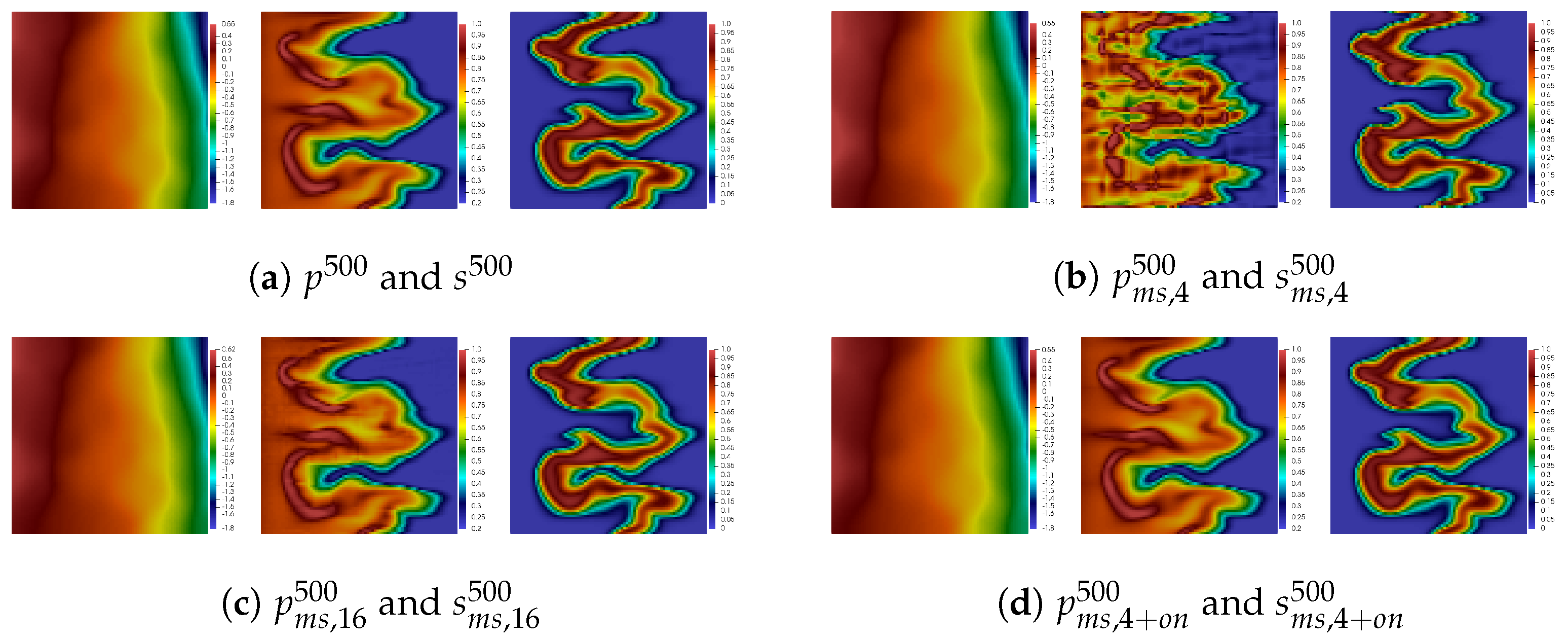
In Figure 8, Figure 9, Figure 10 and Figure 11, we depict results of numerical simulations at a final time for Tests 1, 2, 3 and 4 for Heterogeneity-1. In the first column, we depict a fine grid solution. The results using the presented multiscale method using four multiscale basis functions without and with online correction are depicted in the second and third columns. In the last fourth column, we demonstrate the results of the multiscale method using 16 multiscale basis functions without online correction. From the presented results of fine grid simulations, we observe a strong influence of the polymer concentration on the final saturation (see Figure 8 and Figure 11 for Tests 1 and 4). The effect of the polymer injection duration is represented in Figure 9 and Figure 10 for Tests 2 and 3.

Figure 8. Heterogeneity-1. Results of numerical simulations at final time for Test 1.

Figure 9. Heterogeneity-1. Results of numerical simulations at final time for Test 2.

Figure 10. Heterogeneity-1. Results of numerical simulations at final time for Test 3.

Figure 11. Heterogeneity-1. Results of numerical simulations at final time for Test 4.

In Figure 8, the results illustrate the accuracy of the presented multiscale solver for the solution of the two-phase flow problem (Test 1, no polymer injection). From the second and fourth columns, we observe the slight influence of a number of multiscale basis functions on the pressure field. However, the explicitly calculated fine grid saturation has a considerable difference. Moreover, the presented approach with local residual-based correction provides excellent results for the case with four multiscale basis functions.

In Figure 9 and Figure 10, we consider Tests 2 and 3, where polymer injection is given at the first 100 and 200 time steps, respectively (total number of time steps is 500). The concentration and pressure fields look accurate for the case with 4 and 16 multiscale basis functions without correction. However, the saturation field is susceptible to the number of bases, and the four functions are insufficient for obtaining good results. However, the proposed local online correction provides great results.

Numerical results for the Test 4 are presented in Figure 11. Similarly to the previous test problems, we observe a considerable influence of the number of basis functions on the final saturation solution.

Next, we consider test cases for Heterogeneity-2. In Table 4, we present relative errors for an $8\times 8$ coarse grid. We observe good results for all test cases with a sufficient number of multiscale basis functions for the pressure that can provide good approximations of fluxes. Moreover, we observe the effect of the online correction step that works great with a sufficient number of multiscale basis functions for all test cases of the polymer injection for Heterogeneity-2. In the channelized permeability field, we observe significant errors for the multiscale method without a correction step compared. However, online correction leads to very accurate results with fewer basis functions. For example, using the online correction step, we have $2.5\%$ of error for concentration using four multiscale basis functions and $0.7\%$ using eight multiscale basis functions in the Test 2 for Heterogeneity-1. For Heterogeneity-2, we have $1.4\%$ of error for concentration using four multiscale basis functions and $0.2\%$ using eight multiscale basis functions in the Test 2.

Table 4. Heterogeneity-2. Relative errors at final time. Coarse mesh $8\times 8$.

	${\mathit{e}}_{\mathit{p}}$ (%)	${\mathit{e}}_{{\mathit{u}}_{\mathit{w}}}$ (%)	${\mathit{e}}_{\mathit{u}}$ (%)	${\mathit{e}}_{\mathit{s}}$ (%)	${\mathit{e}}_{\mathit{c}}$ (%)	${\mathit{e}}_{\mathit{p}}$ (%)	${\mathit{e}}_{{\mathit{u}}_{\mathit{w}}}$ (%)	${\mathit{e}}_{\mathit{u}}$ (%)	${\mathit{e}}_{\mathit{s}}$ (%)	${\mathit{e}}_{\mathit{c}}$ (%)
Test 1
1	19.029	77.975	50.023	48.188	-	4.378	6.139	4.846	6.985	-
2	4.652	40.318	27.244	28.537	-	1.124	1.540	1.337	1.755	-
4	2.309	33.021	22.513	19.120	-	0.543	0.639	0.597	0.647	-
8	1.126	17.683	11.942	9.007	-	0.095	0.126	0.106	0.115	-
12	0.496	6.938	4.762	3.427	-	0.032	0.078	0.056	0.053	-
16	0.234	3.872	2.626	2.074	-	0.007	0.034	0.023	0.024	-
Test 2
1	20.006	78.323	44.569	48.963	87.056	4.782	5.970	4.975	6.521	14.625
2	8.717	45.755	27.707	29.160	59.480	1.116	1.962	1.636	2.565	4.144
4	5.800	36.804	23.224	21.672	40.370	0.576	0.812	0.714	0.866	1.430
8	0.966	20.272	14.158	10.964	16.776	0.113	0.157	0.133	0.159	0.254
12	0.542	7.785	5.545	4.989	8.148	0.037	0.072	0.053	0.062	0.096
16	0.271	4.869	3.418	3.535	5.810	0.008	0.031	0.022	0.031	0.048
Test 3
1	19.009	80.733	45.054	48.508	65.171	4.633	5.665	4.624	5.224	11.639
2	7.550	39.566	23.701	29.321	46.726	1.102	2.064	1.640	1.955	3.187
4	6.218	36.561	22.308	20.294	29.820	0.549	0.768	0.653	0.705	1.093
8	1.370	19.596	13.304	10.503	11.522	0.120	0.167	0.139	0.136	0.184
12	0.399	7.697	5.317	5.161	5.750	0.038	0.082	0.061	0.052	0.075
16	0.261	5.780	3.949	3.658	4.081	0.013	0.041	0.029	0.028	0.040
Test 4
1	20.039	86.238	43.783	43.754	33.495	4.253	4.123	3.643	3.992	3.986
2	4.767	39.402	16.693	28.987	21.471	1.046	1.111	1.078	1.039	0.733
4	2.530	30.716	13.495	17.775	10.269	0.446	0.427	0.502	0.416	0.280
8	0.838	16.162	8.371	8.503	4.112	0.082	0.125	0.096	0.096	0.055
12	0.431	8.588	4.391	4.385	2.291	0.029	0.070	0.043	0.046	0.031
16	0.210	4.687	2.339	2.614	1.438	0.009	0.031	0.018	0.021	0.015

For the multiscale solution of the pressure equation, we observe that the online local residual-based correction provides an excellent error reduction for the velocity field, leading to accurate calculations of the saturation and concentration problems. From the presented results in Table 1, Table 2 and Table 3, we also observe the effect of the coarse grid size and a number of local multiscale basis functions on the method accuracy, where a finer coarse grid leads to the minor error with a smaller number of basis functions. The effect of the heterogeneity field on the method accuracy is investigated.

4.2. Splitted Multiscale Approach

We present results for the splitted multiscale approach, where we decouple part of the equation related to the first basis function or primary continuum.

In Table 5 and Table 6, we present the errors at the final time for a splitted multiscale approach. The calculation is performed on the $8\times 8$ coarse grid. By system splitting, we separate the equations for the first and all other continua. The resulting errors are minor for the pressure field but lead to more significant errors for concentrations in the case without online correction. For example, we have $e_p=1.8\%$, $e_{u_w}=10.4\%$, $e_s=6.3$ and $e_c=6.8$ for the regular coupled multiscale method, and $e_p=2.2\%$, $e_{u_w}=12.6\%$, $e_s=6.6$ and $e_c=7.1$ for the splitted multiscale method in Test 3 with Heterogeneity-1 (see Table 2 and Table 5). In Test 3 for Heterogeneity-2, we have $e_p=1.3\%$, $e_{u_w}=19.5\%$, $e_s=10.5$ and $e_c=11.5$ for the regular coupled multiscale method, and $e_p=1.6\%$, $e_{u_w}=19.2\%$, $e_s=10.6$ and $e_c=12.2$ for the splitted multiscale method in Test 3 (see Table 4 and Table 6) However, we observe accurate results for the case with online correction. In this case, correction reduces the error of multiscale offline basis functions and is remarkable for the splitting approach. Therefore, we can use a splitting approach for the polymer flooding processes with an online correction step to reduce errors. Note that the error behavior is similar for two types of heterogeneity.

Table 5. Heterogeneity-1. Splitted multiscale approach on $8\times 8$ coarse grid.

	${\mathit{e}}_{\mathit{p}}$ (%)	${\mathit{e}}_{{\mathit{u}}_{\mathit{w}}}$ (%)	${\mathit{e}}_{\mathit{u}}$ (%)	${\mathit{e}}_{\mathit{s}}$ (%)	${\mathit{e}}_{\mathit{c}}$ (%)	${\mathit{e}}_{\mathit{p}}$ (%)	${\mathit{e}}_{{\mathit{u}}_{\mathit{w}}}$ (%)	${\mathit{e}}_{\mathit{u}}$ (%)	${\mathit{e}}_{\mathit{s}}$ (%)	${\mathit{e}}_{\mathit{c}}$ (%)
Test 1
2	3.848	34.659	26.806	20.415	-	1.187	2.050	1.616	1.915	-
4	1.597	15.840	12.389	10.629	-	0.665	1.009	0.811	0.913	-
8	0.527	9.556	7.400	5.784	-	0.162	0.372	0.286	0.295	-
12	0.171	2.450	1.999	1.621	-	0.062	0.120	0.086	0.109	-
16	0.104	2.797	2.107	1.983	-	0.023	0.055	0.039	0.057	-
Test 2
2	14.116	41.532	32.263	25.288	47.367	1.177	3.180	2.642	2.869	6.238
4	3.613	18.329	15.111	12.358	21.561	0.538	1.232	1.021	1.146	2.345
8	1.070	12.200	10.249	6.378	8.086	0.151	0.432	0.362	0.362	0.583
12	0.295	3.991	3.424	2.433	3.391	0.089	0.276	0.220	0.240	0.496
16	0.205	3.348	2.808	2.024	2.667	0.041	0.147	0.118	0.140	0.335
Test 3
2	14.190	37.264	27.823	24.349	31.712	0.559	3.017	2.464	2.001	3.849
4	5.506	21.872	17.424	13.359	14.210	0.294	1.492	1.213	0.970	1.857
8	2.282	12.681	10.432	6.682	7.106	0.117	0.428	0.342	0.311	0.454
12	0.378	5.974	4.931	2.685	2.791	0.075	0.339	0.275	0.244	0.354
16	0.182	4.541	3.691	2.197	2.340	0.047	0.182	0.151	0.153	0.220
Test 4
2	4.428	27.450	16.845	18.224	11.254	1.783	2.182	1.480	1.922	1.310
4	1.980	16.087	10.147	11.338	6.198	0.909	1.153	0.777	0.922	0.568
8	0.942	8.668	5.833	5.830	2.204	0.275	0.392	0.256	0.309	0.191
12	0.128	1.915	1.471	1.363	0.517	0.026	0.051	0.029	0.038	0.027
16	0.060	1.711	1.079	1.073	0.325	0.010	0.020	0.011	0.016	0.012

Table 6. Heterogeneity-2. Splitted multiscale approach on $8\times 8$ coarse grid.

	${\mathit{e}}_{\mathit{p}}$ (%)	${\mathit{e}}_{{\mathit{u}}_{\mathit{w}}}$ (%)	${\mathit{e}}_{\mathit{u}}$ (%)	${\mathit{e}}_{\mathit{s}}$ (%)	${\mathit{e}}_{\mathit{c}}$ (%)	${\mathit{e}}_{\mathit{p}}$ (%)	${\mathit{e}}_{{\mathit{u}}_{\mathit{w}}}$ (%)	${\mathit{e}}_{\mathit{u}}$ (%)	${\mathit{e}}_{\mathit{s}}$ (%)	${\mathit{e}}_{\mathit{c}}$ (%)
Test 1
2	4.652	40.327	27.251	28.539	-	1.122	1.540	1.336	1.752	-
4	2.321	33.004	22.495	19.156	-	0.541	0.637	0.595	0.642	-
8	1.097	16.976	11.409	9.153	-	0.093	0.127	0.106	0.113	-
12	0.517	6.843	4.701	3.421	-	0.032	0.082	0.058	0.055	-
16	0.343	4.588	3.109	2.355	-	0.006	0.037	0.025	0.024	-
Test 2
2	8.701	45.677	27.666	29.163	59.508	1.114	1.960	1.635	2.559	4.133
4	5.704	36.405	22.958	21.634	40.434	0.576	0.805	0.709	0.855	1.426
8	0.975	19.807	13.812	11.287	18.225	0.107	0.152	0.127	0.156	0.264
12	0.605	7.930	5.653	5.111	8.427	0.036	0.078	0.058	0.064	0.090
16	0.369	5.929	4.180	3.998	6.795	0.010	0.035	0.024	0.028	0.044
Test 3
2	7.584	39.525	23.658	29.316	46.754	1.102	2.056	1.635	1.949	3.180
4	6.285	36.931	22.513	20.342	29.911	0.548	0.765	0.650	0.694	1.091
8	1.642	19.240	12.967	10.697	12.277	0.121	0.186	0.148	0.138	0.191
12	0.408	8.578	5.962	5.454	6.159	0.036	0.081	0.060	0.048	0.068
16	0.325	7.507	5.113	4.447	5.182	0.013	0.049	0.034	0.029	0.040
Test 4
2	4.769	39.406	16.692	28.986	21.467	1.047	1.113	1.079	1.040	0.734
4	2.532	30.683	13.490	17.766	10.347	0.448	0.428	0.502	0.418	0.282
8	0.824	16.337	8.396	8.704	4.060	0.084	0.127	0.099	0.101	0.055
12	0.484	8.169	4.182	4.341	2.328	0.031	0.069	0.044	0.046	0.031
16	0.287	5.865	2.847	3.101	1.807	0.012	0.032	0.019	0.023	0.017

4.3. Loose Coupling

Finally, we combine a multiscale splitting approach with a loose coupling technique for transport and pressure equations. We consider the traditional and splitted multiscale approaches with two values of the loose coupling parameter $n_p=2$ and 5.

In Table 7 and Table 8, we present results for the loose coupling approach for Heterogeneity-1 and Heterogeneity-2. In the loose coupling approach, we calculate pressure if the remainder of dividing n by 2 is equal to zero. For $n_p=2$, we observe good results with almost the same errors except Test 2, where the minimum error for concentration was 0.03% using 16 multiscale basis functions with online correction compared with 1.9% for the case for loose coupling. We obtain a slightly bigger error by comparing traditional coupled and splitted multiscale approaches. Overall, we can state that the results with online correction work great for the splitted multiscale method with loose coupling. Moreover, we observe that the loose coupling works better for Heterogeneity-2 with more minor errors.

Table 7. Heterogeneity-1. Loose coupling with $n_p=2$ on $8\times 8$ coarse grid.

	${\mathit{e}}_{\mathit{p}}$ (%)	${\mathit{e}}_{{\mathit{u}}_{\mathit{w}}}$ (%)	${\mathit{e}}_{\mathit{u}}$ (%)	${\mathit{e}}_{\mathit{s}}$ (%)	${\mathit{e}}_{\mathit{c}}$ (%)	${\mathit{e}}_{\mathit{p}}$ (%)	${\mathit{e}}_{{\mathit{u}}_{\mathit{w}}}$ (%)	${\mathit{e}}_{\mathit{u}}$ (%)	${\mathit{e}}_{\mathit{s}}$ (%)	${\mathit{e}}_{\mathit{c}}$ (%)
Test 1 (ms-coupled)
2	3.956	34.595	26.782	20.446	-	1.260	2.165	1.724	2.023	-
4	1.553	15.873	12.403	10.650	-	0.590	1.108	0.879	0.902	-
8	0.511	9.652	7.448	5.986	-	0.104	0.438	0.321	0.286	-
12	0.136	1.918	1.679	1.315	-	0.138	0.226	0.141	0.190	-
16	0.130	1.648	1.247	1.030	-	0.141	0.215	0.133	0.189	-
Test 2 (ms-coupled)
2	14.047	41.152	31.959	25.288	47.270	1.276	3.025	2.558	2.945	5.836
4	3.742	18.225	15.024	12.400	21.506	0.480	1.293	1.098	1.030	2.033
8	0.820	11.283	9.511	6.353	7.680	0.180	1.026	0.812	0.596	1.664
12	0.257	2.545	2.241	1.939	2.653	0.213	1.031	0.789	0.691	1.966
16	0.231	1.970	1.593	1.407	2.403	0.215	1.021	0.777	0.697	1.987
Test 3 (ms-coupled)
2	14.088	37.548	28.035	24.425	32.077	0.660	3.326	2.737	2.127	4.246
4	5.589	21.641	17.183	13.405	14.167	0.432	1.500	1.259	0.851	1.737
8	1.865	10.186	8.440	6.387	6.752	0.238	0.852	0.701	0.424	0.777
12	0.313	3.411	2.835	2.010	2.140	0.244	0.985	0.790	0.540	0.965
16	0.260	2.562	2.065	1.449	1.569	0.245	0.996	0.797	0.551	0.985
Test 4 (ms-coupled)
2	4.447	27.446	16.848	18.220	11.252	1.746	2.146	1.484	1.861	1.281
4	1.977	16.084	10.152	11.326	6.185	0.879	1.123	0.779	0.873	0.555
8	0.890	8.841	5.935	5.955	2.224	0.224	0.365	0.252	0.258	0.163
12	0.091	1.901	1.470	1.324	0.324	0.025	0.106	0.042	0.074	0.050
16	0.054	1.582	0.987	0.953	0.230	0.030	0.104	0.035	0.079	0.052
	$e_p$ (%)	$e_{u_w}$ (%)	$e_u$ (%)	$e_s$ (%)	$e_c$ (%)	$e_p$ (%)	$e_{u_w}$ (%)	$e_u$ (%)	$e_s$ (%)	$e_c$ (%)
Test 1 (ms-splitted)
2	3.688	34.591	26.711	20.284	-	0.884	2.073	1.603	1.680	-
4	1.507	15.808	12.356	10.583	-	0.505	1.079	0.840	0.829	-
8	0.494	9.933	7.711	5.804	-	0.249	0.550	0.396	0.399	-
12	0.553	7.720	5.562	5.083	-	0.236	0.348	0.225	0.319	-
16	0.229	4.620	3.588	3.153	-	0.175	0.266	0.163	0.250	-
Test 2 (ms-splitted)
2	14.486	41.518	32.163	25.462	47.022	0.842	2.791	2.374	2.207	4.515
4	3.853	18.190	15.014	12.354	21.289	0.402	1.274	1.067	0.935	1.871
8	2.020	13.398	11.054	6.974	8.473	0.354	1.388	1.080	0.934	2.303
12	0.951	8.940	7.208	4.823	8.461	0.334	1.350	1.031	0.983	2.649
16	0.566	5.761	4.780	3.425	5.085	0.268	1.191	0.906	0.859	2.428
Test 3 (ms-splitted)
2	14.412	37.491	27.963	24.590	31.746	0.659	2.447	2.048	1.432	2.684
4	5.698	21.643	17.236	13.486	14.113	0.414	1.305	1.087	0.742	1.376
8	3.034	14.970	11.859	7.599	8.008	0.279	1.285	1.024	0.699	1.098
12	1.053	12.763	10.282	5.429	9.891	0.306	1.409	1.121	0.835	1.444
16	0.613	8.750	7.112	4.097	5.838	0.297	1.223	0.979	0.722	1.286
Test 4 (ms-splitted)
2	4.414	27.431	16.844	18.221	11.312	1.782	2.147	1.483	1.884	1.336
4	2.013	16.099	10.150	11.352	6.224	0.899	1.130	0.783	0.883	0.580
8	0.992	8.572	5.763	5.857	2.323	0.293	0.386	0.273	0.294	0.229
12	0.151	2.399	1.775	1.524	0.641	0.047	0.102	0.050	0.076	0.072
16	0.080	1.903	1.178	1.245	0.478	0.030	0.103	0.036	0.078	0.056

Table 8. Heterogeneity-2. Loose coupling with $n_p=2$ on $8\times 8$ coarse grid.

	${\mathit{e}}_{\mathit{p}}$ (%)	${\mathit{e}}_{{\mathit{u}}_{\mathit{w}}}$ (%)	${\mathit{e}}_{\mathit{u}}$ (%)	${\mathit{e}}_{\mathit{s}}$ (%)	${\mathit{e}}_{\mathit{c}}$ (%)	${\mathit{e}}_{\mathit{p}}$ (%)	${\mathit{e}}_{{\mathit{u}}_{\mathit{w}}}$ (%)	${\mathit{e}}_{\mathit{u}}$ (%)	${\mathit{e}}_{\mathit{s}}$ (%)	${\mathit{e}}_{\mathit{c}}$ (%)
Test 1 (ms-coupled)
2	4.658	40.333	27.251	28.552	-	1.107	1.547	1.343	1.710	-
4	2.321	33.025	22.507	19.113	-	0.528	0.660	0.607	0.626	-
8	1.141	17.698	11.947	9.013	-	0.085	0.168	0.123	0.160	-
12	0.501	6.942	4.761	3.430	-	0.037	0.111	0.064	0.116	-
16	0.239	3.874	2.624	2.082	-	0.033	0.100	0.047	0.114	-
Test 2 (ms-coupled)
2	8.671	45.658	27.689	29.150	59.333	1.139	1.808	1.582	2.360	3.489
4	5.755	36.838	23.264	21.698	40.192	0.597	0.608	0.625	0.734	0.970
8	0.981	20.448	14.287	10.960	16.660	0.148	0.455	0.308	0.389	0.757
12	0.574	7.809	5.559	4.992	8.133	0.084	0.494	0.322	0.390	0.826
16	0.313	4.844	3.387	3.564	5.871	0.072	0.509	0.328	0.404	0.856
Test 3 (ms-coupled)
2	7.565	39.563	23.671	29.304	46.644	1.121	1.975	1.644	1.814	2.889
4	6.173	36.609	22.330	20.309	29.767	0.569	0.633	0.623	0.630	0.869
8	1.366	19.758	13.410	10.542	11.466	0.152	0.473	0.306	0.359	0.409
12	0.409	7.763	5.358	5.208	5.721	0.076	0.479	0.295	0.348	0.432
16	0.278	5.769	3.932	3.713	4.052	0.061	0.490	0.295	0.356	0.443
Test 4 (ms-coupled)
2	4.768	39.385	16.692	28.984	21.482	1.049	1.097	1.081	1.022	0.727
4	2.528	30.706	13.496	17.766	10.265	0.450	0.403	0.502	0.404	0.277
8	0.841	16.171	8.374	8.501	4.109	0.087	0.137	0.097	0.116	0.073
12	0.435	8.602	4.395	4.389	2.301	0.034	0.101	0.049	0.067	0.057
16	0.214	4.705	2.345	2.619	1.451	0.014	0.080	0.028	0.057	0.047
	$e_p$ (%)	$e_{u_w}$ (%)	$e_u$ (%)	$e_s$ (%)	$e_c$ (%)	$e_p$ (%)	$e_{u_w}$ (%)	$e_u$ (%)	$e_s$ (%)	$e_c$ (%)
Test 1 (ms-splitted)
2	4.656	40.349	27.265	28.556	-	1.103	1.549	1.343	1.705	-
4	2.343	33.003	22.479	19.191	-	0.524	0.655	0.602	0.618	-
8	1.114	17.274	11.594	9.424	-	0.081	0.172	0.123	0.164	-
12	0.556	6.475	4.461	3.429	-	0.039	0.116	0.065	0.120	-
16	0.397	5.115	3.458	2.514	-	0.036	0.105	0.049	0.120	-
Test 2 (ms-splitted)
2	8.636	45.501	27.606	29.154	59.371	1.135	1.807	1.582	2.349	3.469
4	5.674	36.333	22.930	21.682	40.276	0.596	0.601	0.619	0.717	0.959
8	0.987	19.342	13.488	11.447	18.764	0.140	0.469	0.319	0.388	0.748
12	0.658	7.681	5.472	5.144	8.512	0.084	0.504	0.330	0.395	0.839
16	0.429	6.544	4.620	4.181	7.025	0.072	0.510	0.328	0.409	0.863
Test 3 (ms-splitted)
2	7.629	39.488	23.598	29.294	46.705	1.121	1.959	1.635	1.804	2.877
4	6.243	37.209	22.605	20.428	29.831	0.567	0.611	0.608	0.612	0.868
8	1.748	19.603	13.245	10.943	12.742	0.152	0.468	0.298	0.364	0.411
12	0.433	8.333	5.777	5.517	6.177	0.069	0.480	0.291	0.352	0.447
16	0.367	8.206	5.603	4.664	5.261	0.057	0.475	0.279	0.359	0.451
Test 4 (ms-splitted)
2	4.773	39.393	16.690	28.983	21.476	1.051	1.100	1.082	1.023	0.728
4	2.535	30.619	13.485	17.751	10.464	0.453	0.405	0.503	0.407	0.281
8	0.831	16.593	8.524	8.889	4.139	0.092	0.140	0.102	0.121	0.073
12	0.523	7.936	4.070	4.344	2.344	0.038	0.098	0.051	0.066	0.056
16	0.306	6.291	3.069	3.206	1.820	0.019	0.080	0.030	0.058	0.048

In Table 9 and Table 10, we present results for the loose coupling approach, where we calculate pressure if dividing n by 5 equals zero. Therefore, with the total number of iterations of 500, we calculate pressure only 100 times. From the results, we observe that the errors highly vary for different test cases; in the Tests 2 and 3, the errors increase significantly for both coupled and splitted multiscale approaches.

Table 9. Heterogeneity-1. Loose coupling with $n_p=5$ on $8\times 8$ coarse grid.

	${\mathit{e}}_{\mathit{p}}$ (%)	${\mathit{e}}_{{\mathit{u}}_{\mathit{w}}}$ (%)	${\mathit{e}}_{\mathit{u}}$ (%)	${\mathit{e}}_{\mathit{s}}$ (%)	${\mathit{e}}_{\mathit{c}}$ (%)	${\mathit{e}}_{\mathit{p}}$ (%)	${\mathit{e}}_{{\mathit{u}}_{\mathit{w}}}$ (%)	${\mathit{e}}_{\mathit{u}}$ (%)	${\mathit{e}}_{\mathit{s}}$ (%)	${\mathit{e}}_{\mathit{c}}$ (%)
Test 1 (ms-coupled)
2	3.839	34.483	26.671	20.324	-	0.903	2.352	1.834	1.845	-
4	1.397	15.878	12.375	10.616	-	0.317	1.461	1.071	0.947	-
8	0.405	9.650	7.422	5.982	-	0.422	0.929	0.603	0.684	-
12	0.526	2.080	1.745	1.497	-	0.555	0.820	0.507	0.733	-
16	0.536	1.829	1.335	1.257	-	0.559	0.811	0.501	0.733	-
Test 2 (ms-coupled)
2	14.271	41.170	31.941	25.544	47.273	1.015	3.563	2.959	2.675	5.637
4	4.327	18.135	14.916	12.642	21.173	0.600	3.454	2.693	2.235	6.128
8	1.276	11.648	9.717	6.847	9.553	0.743	3.791	2.904	2.534	7.050
12	0.831	4.302	3.457	3.212	7.286	0.820	3.837	2.918	2.682	7.391
16	0.828	4.087	3.161	2.926	7.428	0.823	3.828	2.909	2.689	7.412
Test 3 (ms-coupled)
2	14.018	37.921	28.337	24.727	32.613	1.101	3.926	3.300	2.007	3.979
4	6.077	21.024	16.565	13.807	14.473	1.034	3.436	2.827	1.771	3.266
8	2.058	9.884	8.105	6.864	7.275	0.912	3.572	2.871	2.010	3.561
12	0.939	4.766	3.859	3.009	4.274	0.934	3.755	2.997	2.176	3.850
16	0.936	4.266	3.415	2.584	3.967	0.936	3.767	3.005	2.186	3.870
Test 4 (ms-coupled)
2	4.454	27.414	16.854	18.209	11.342	1.711	2.068	1.496	1.739	1.311
4	2.027	16.094	10.163	11.330	6.219	0.848	1.103	0.799	0.792	0.604
8	0.875	8.825	5.931	5.935	2.239	0.210	0.483	0.289	0.302	0.266
12	0.143	1.945	1.477	1.355	0.384	0.123	0.409	0.135	0.308	0.206
16	0.136	1.637	0.998	1.000	0.300	0.128	0.412	0.133	0.315	0.209
	$e_p$ (%)	$e_{u_w}$ (%)	$e_u$ (%)	$e_s$ (%)	$e_c$ (%)	$e_p$ (%)	$e_{u_w}$ (%)	$e_u$ (%)	$e_s$ (%)	$e_c$ (%)
Test 1 (ms-splitted)
2	3.743	35.053	26.953	20.291	-	0.647	2.581	1.863	1.561	-
4	1.403	15.745	12.279	10.513	-	0.432	1.518	1.066	0.976	-
8	1.041	10.491	8.104	6.446	-	0.856	1.290	0.870	1.063	-
12	1.635	14.223	10.691	9.278	-	0.759	1.068	0.670	0.985	-
16	0.763	7.826	5.924	4.953	-	0.638	0.920	0.564	0.862	-
Test 2 (ms-splitted)
2	15.991	41.648	32.038	26.145	47.332	0.994	4.927	3.888	3.483	8.260
4	4.716	18.225	15.036	12.690	21.466	0.767	3.966	3.048	2.694	7.370
8	3.275	15.592	12.575	8.620	13.167	1.166	4.595	3.501	3.251	8.450
12	2.292	16.484	12.906	9.608	22.781	1.077	4.495	3.415	3.261	8.777
16	2.512	18.359	14.631	9.285	20.856	0.949	4.200	3.190	3.035	8.350
Test 3 (ms-splitted)
2	15.718	38.461	28.607	25.535	32.504	1.560	5.430	4.331	3.100	5.375
4	6.373	21.196	16.813	14.082	14.378	1.067	3.857	3.095	2.119	3.792
8	3.901	16.874	13.132	9.182	10.723	0.982	4.467	3.520	2.579	4.350
12	2.392	19.297	14.695	10.034	13.531	1.053	4.566	3.615	2.728	4.769
16	2.022	21.048	16.398	9.582	11.754	1.048	4.240	3.378	2.536	4.502
Test 4 (ms-splitted)
2	4.384	27.387	16.846	18.222	11.544	1.823	2.088	1.507	1.818	1.464
4	2.124	16.152	10.175	11.406	6.339	0.907	1.110	0.811	0.816	0.665
8	1.281	8.865	6.007	6.055	2.755	0.422	0.478	0.359	0.373	0.417
12	0.295	5.446	3.603	2.482	1.150	0.168	0.372	0.149	0.296	0.258
16	0.245	3.337	1.994	2.481	1.507	0.129	0.408	0.135	0.311	0.219

Table 10. Heterogeneity-2. Loose coupling with $n_p=5$ on $8\times 8$ coarse grid.

	${\mathit{e}}_{\mathit{p}}$ (%)	${\mathit{e}}_{{\mathit{u}}_{\mathit{w}}}$ (%)	${\mathit{e}}_{\mathit{u}}$ (%)	${\mathit{e}}_{\mathit{s}}$ (%)	${\mathit{e}}_{\mathit{c}}$ (%)	${\mathit{e}}_{\mathit{p}}$ (%)	${\mathit{e}}_{{\mathit{u}}_{\mathit{w}}}$ (%)	${\mathit{e}}_{\mathit{u}}$ (%)	${\mathit{e}}_{\mathit{s}}$ (%)	${\mathit{e}}_{\mathit{c}}$ (%)
Test 1 (ms-coupled)
2	4.677	40.382	27.277	28.598	-	1.062	1.602	1.370	1.621	-
4	2.357	33.039	22.488	19.092	-	0.494	0.784	0.651	0.685	-
8	1.191	17.760	11.969	9.041	-	0.123	0.410	0.222	0.465	-
12	0.528	6.962	4.759	3.461	-	0.124	0.367	0.173	0.445	-
16	0.276	3.894	2.623	2.144	-	0.131	0.374	0.174	0.451	-
Test 2 (ms-coupled)
2	8.534	45.405	27.646	29.133	58.920	1.235	2.172	1.817	2.160	2.655
4	5.617	36.948	23.384	21.795	39.730	0.704	1.601	1.142	1.382	2.555
8	1.052	21.072	14.729	11.036	16.597	0.330	1.914	1.235	1.565	3.251
12	0.707	8.052	5.696	5.192	8.591	0.287	1.965	1.265	1.584	3.335
16	0.480	5.051	3.461	3.902	6.707	0.278	1.982	1.273	1.600	3.365
Test 3 (ms-coupled)
2	7.605	39.580	23.586	29.264	46.439	1.201	2.370	1.938	1.806	2.376
4	6.040	36.774	22.398	20.375	29.643	0.661	1.624	1.138	1.271	1.383
8	1.359	20.285	13.752	10.718	11.419	0.296	1.894	1.154	1.401	1.712
12	0.484	8.118	5.564	5.474	5.850	0.236	1.915	1.162	1.404	1.754
16	0.382	5.980	4.014	4.055	4.262	0.226	1.929	1.164	1.414	1.767
Test 4 (ms-coupled)
2	4.770	39.331	16.690	28.973	21.516	1.063	1.079	1.090	0.989	0.728
4	2.522	30.675	13.498	17.739	10.258	0.466	0.409	0.507	0.414	0.306
8	0.853	16.197	8.387	8.498	4.104	0.109	0.306	0.123	0.247	0.180
12	0.454	8.645	4.409	4.403	2.337	0.058	0.301	0.098	0.216	0.175
16	0.233	4.764	2.365	2.642	1.495	0.041	0.295	0.087	0.217	0.168
	$e_p$ (%)	$e_{u_w}$ (%)	$e_u$ (%)	$e_s$ (%)	$e_c$ (%)	$e_p$ (%)	$e_{u_w}$ (%)	$e_u$ (%)	$e_s$ (%)	$e_c$ (%)
Test 1 (ms-splitted)
2	4.674	40.423	27.318	28.615	-	1.053	1.605	1.369	1.610	-
4	2.397	33.122	22.522	19.287	-	0.487	0.774	0.640	0.678	-
8	1.172	17.717	11.882	9.787	-	0.125	0.420	0.226	0.474	-
12	0.655	6.201	4.262	3.606	-	0.131	0.372	0.172	0.455	-
16	0.485	5.899	3.965	2.795	-	0.140	0.383	0.176	0.464	-
Test 2 (ms-splitted)
2	8.453	44.973	27.410	29.128	58.946	1.227	2.198	1.834	2.141	2.620
4	5.737	36.715	23.094	21.875	39.823	0.700	1.621	1.157	1.367	2.508
8	1.036	19.588	13.670	11.840	19.315	0.321	1.929	1.251	1.565	3.234
12	0.830	7.739	5.464	5.451	9.029	0.285	1.973	1.270	1.598	3.363
16	0.613	7.468	5.230	4.617	7.875	0.280	1.975	1.267	1.609	3.379
Test 3 (ms-splitted)
2	7.751	39.424	23.451	29.248	46.582	1.201	2.348	1.921	1.794	2.361
4	6.072	37.800	22.690	20.710	29.653	0.649	1.571	1.093	1.255	1.372
8	1.902	20.224	13.629	11.518	13.578	0.292	1.855	1.114	1.402	1.724
12	0.555	8.403	5.787	5.851	6.361	0.225	1.903	1.141	1.416	1.788
16	0.486	9.014	6.133	5.066	5.430	0.211	1.896	1.130	1.416	1.777
Test 4 (ms-splitted)
2	4.786	39.357	16.685	28.977	21.515	1.067	1.087	1.093	0.991	0.730
4	2.562	30.562	13.489	17.757	10.473	0.474	0.412	0.511	0.420	0.314
8	0.868	17.085	8.753	9.177	4.326	0.123	0.302	0.132	0.246	0.176
12	0.603	7.930	4.063	4.494	2.427	0.066	0.296	0.099	0.214	0.172
16	0.342	6.760	3.319	3.324	1.834	0.048	0.293	0.090	0.215	0.168

For example, in Test 3 for Heterogeneity-1, the concentration errors are $6.8\%$ and $0.6\%$ without and with online correction for eight multiscale functions. For loose coupling with $n_p=5$, we obtain $7.2\%$ and $3.5\%$, respectively. In Test 2 for Heterogeneity-1, the concentration errors are $7.9\%$ and $0.7\%$ without and with online correction for eight multiscale functions. For loose coupling with $n_p=5$, we obtain $9.5\%$ and $7.0\%$, respectively. Overall, we observe a significant effect of the polymer injection schemes on the error behavior of the presented loose coupled splitted multiscale method with online correction, where the most complex case is related to the shorter injection time in Test 2, which leads to the thinner polymer concentration profiles (see Figure 6 and Figure 7). The multiscale method for Tests 2 and 3 works worse than for Test 4 with continuous injection for all methods (Table 9 and Table 10).

5. Conclusions

We considered a polymer flooding process in heterogeneous porous media. A mathematical model is described by equations for the flow and transport processes (saturation and polymer concentration). For the construction of the fine grid approximation, we use a finite volume method with explicit time approximation for the transports and implicit time approximation for the flow processes. The loose coupling was presented to reduce the number of implicit pressure solutions. We presented the coupled and splitted multiscale solver for the nonlinear flow processes in heterogeneous porous media with loose coupling. We constructed a coarse grid approximation using the Generalized Multiscale Finite Element Method with local online correction. The numerical results are presented for two-dimensional model problems with different polymer injection regimes to demonstrate the influence on the method accuracy. We observe

• We investigated the effect of the coarse grid on the method accuracy, where we obtained better results for a finer coarse grid with a more significant number of multiscale basis functions. The polymer injection schemes in test cases significantly affect the multiscale method accuracy. The thinner concentration profiles in Test 2 lead to a more complex case for the multiscale method with more significant errors for the concentration field. However, online correction works well for all coarse grids and significantly improves accuracy.
• The second heterogeneity field leads to the more complex case due to its channelized features. The errors are more extensive for the regular multiscale method without online correction than the Heterogeneity-1, especially for Test 2. However, the online correction works well for both types of permeability fields in all test cases of polymer injection.
• The proposed splitted multiscale method with the online correction step works excellent for all types of polymer injection in Heterogeneity-1 and 2. This splitted approach is promising for future detailed consideration due to the multicontinuum type of decoupling, which separate the primary continuum from others. Furthermore, it relates to splitting the part associated with the convenient homogenization technique, and the other part relates to the local spectral enrichment process.
• We observe that the loose coupling is highly sensitive to the test problems (polymer injection scheme). It works great for the test problem with continuous polymer injection (Test 4) but increases the error for more complex test cases (Tests 2 and 3).

Finally, the sufficient number of multiscale basis functions with online correction for the pressure equation provide reasonable approximations of fluxes for coupled and splitted multiscale methods, leading to accurate calculation of the explicit transport processes.