
Temperature Compensation Algorithm of Air Quality Monitoring Equipment Based on TDLAS


Abstract
1. Introduction
2. Materials and Methods
3. Experimental Apparatus and Process
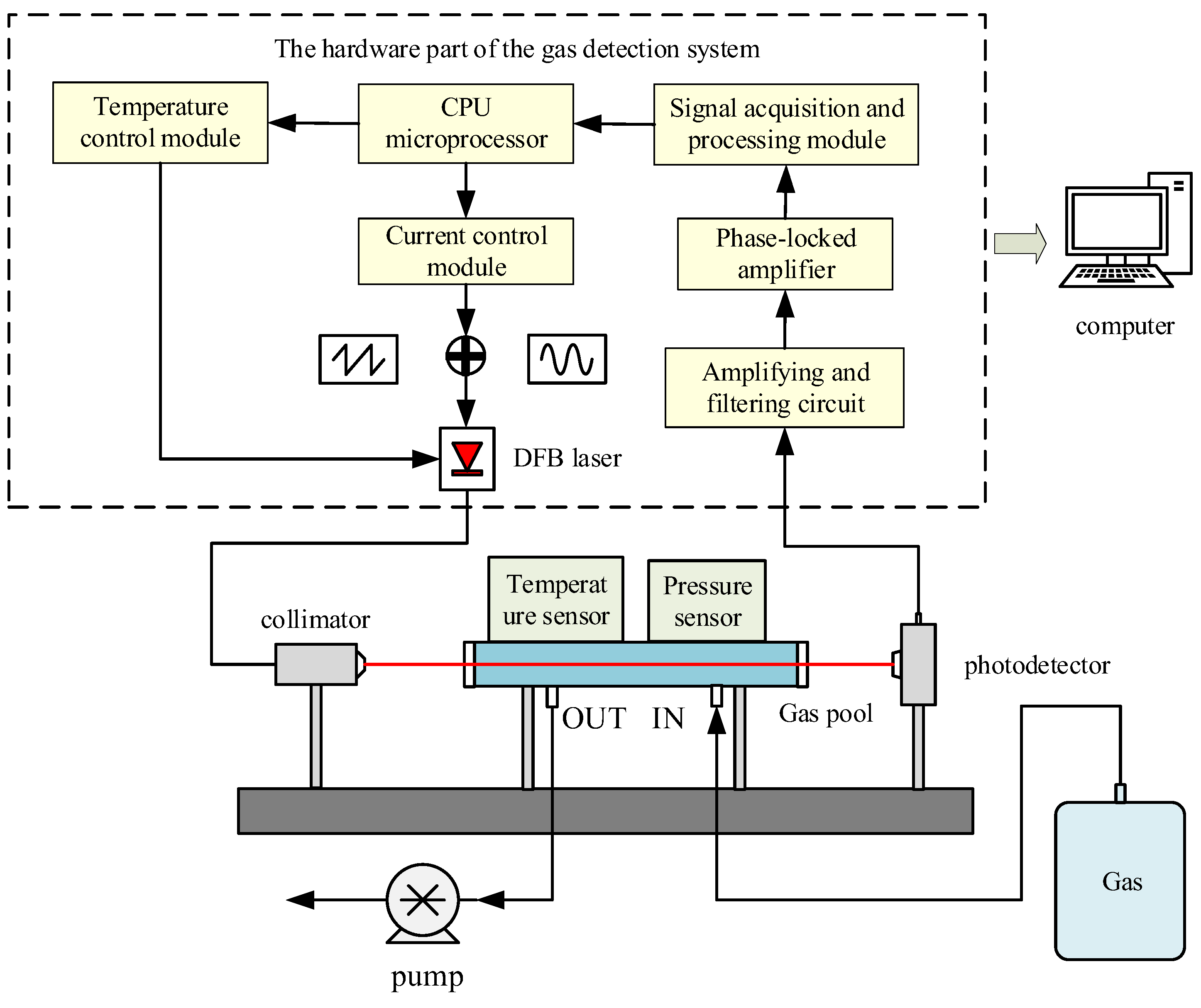
3.1. Construction of Methane Concentration Measurement System
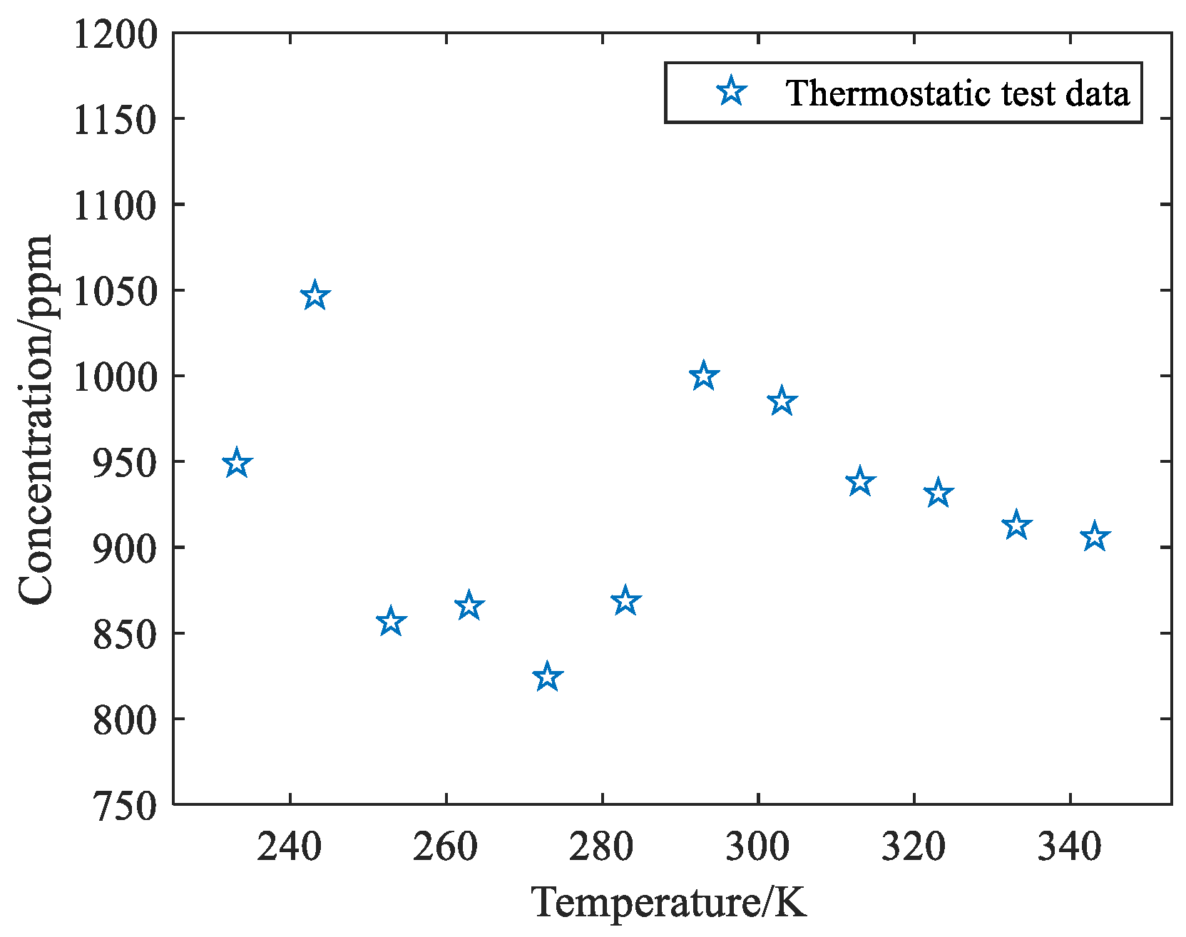
3.2. The Influence of Temperature Change of Gas to Be Measured on Measurement
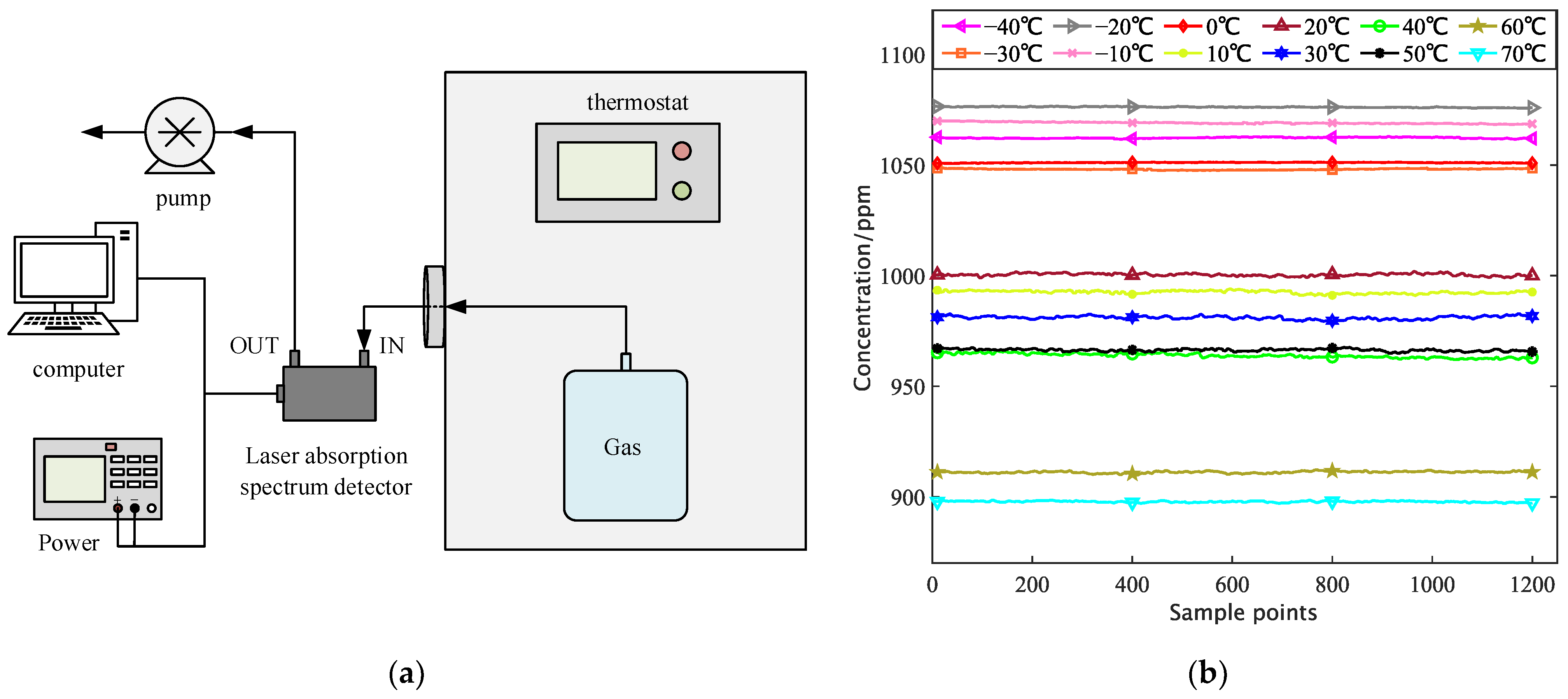
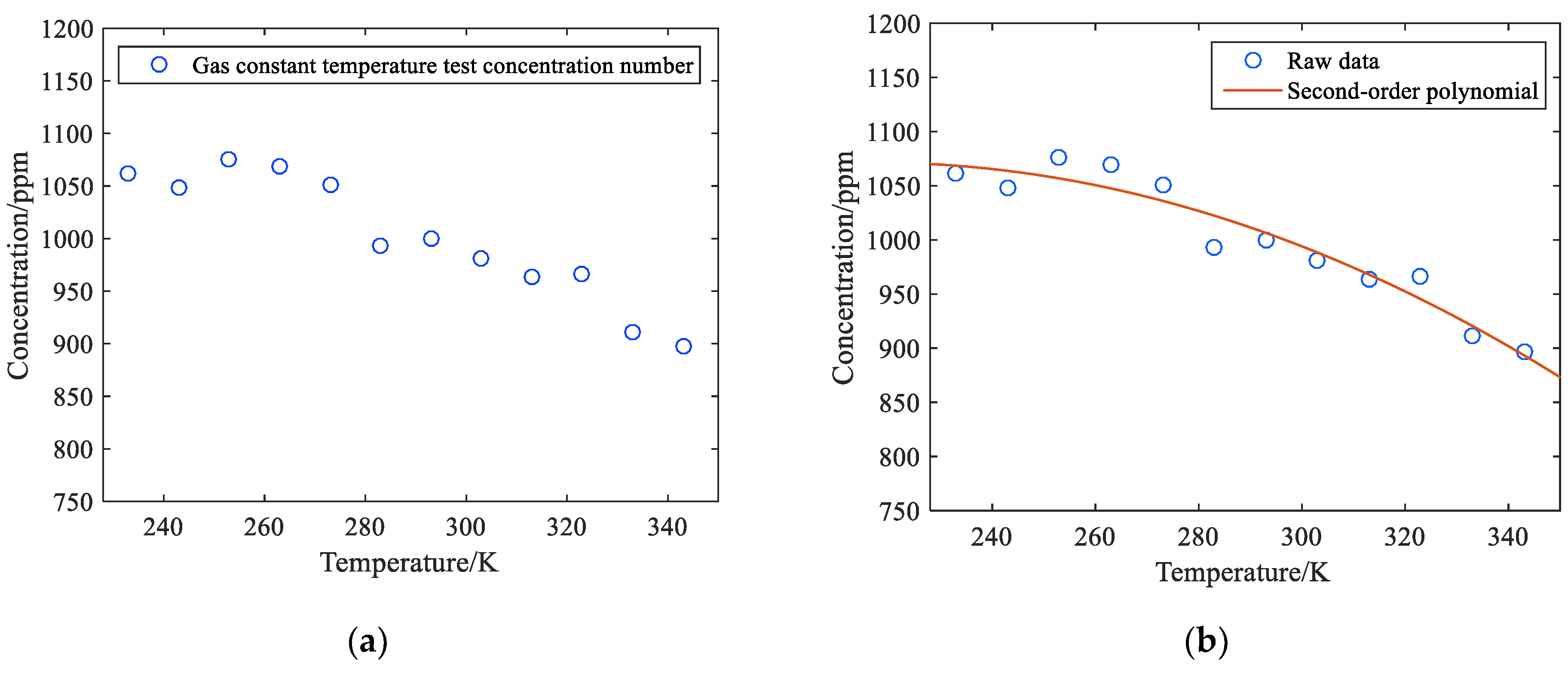
3.3. The Effect of Ambient Temperature Change on Measurement
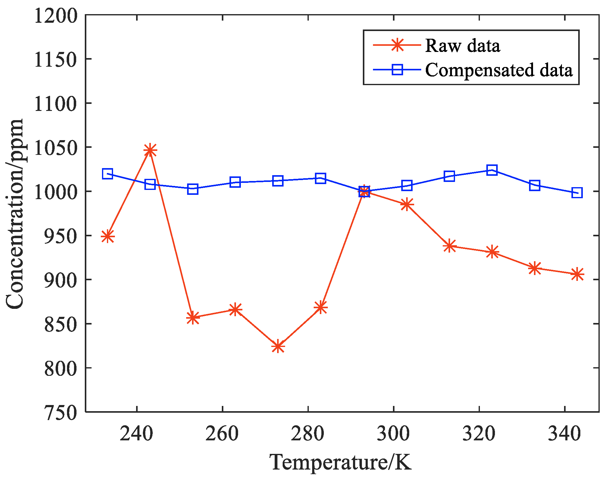
3.4. Correction of Monitoring System under Constant Temperature State of Detector
4. Experimental Results and Analysis
5. Discussion
Author Contributions
Funding
Data Availability Statement
Acknowledgments
Conflicts of Interest
References
- D’Amato, F.; Mazzinghi, P. Methane analyzer based on TDL’s for measurements in the lower stratosphere. Appl. Phys. B 2002, 75, 195–202. [Google Scholar] [CrossRef]
- Iwaszenko, S.; Kalisz, P.; Sota, M. Detection of Natural Gas Leakages Using a Laser-Based Methane Sensor and UAV. Remote Sens. 2021, 13, 510. [Google Scholar] [CrossRef]
- Liu, C.R.; Lian, X.B.; Huang, P.J. Research Review on the spatio-temporal Distribution of Ozone Pollution and Its Causes in China. J. Arid. Meteorol. 2020, 38, 355–361. [Google Scholar]
- Staniaszek, Z.; Griffiths, P.; Folberth, G. The role of future anthropogenic methane emissions in air quality and climate. Npj Clim. Atmos. Sci. 2022, 5, 21. [Google Scholar] [CrossRef]
- Kan, R.F.; Liu, W.Q.; Zhang, Y.J. Tunable diode laser absorption spectrometer monitors the ambient Methane with high sensitivity. Chin. J. Lasers 2005, 32, 1217–1220. [Google Scholar]
- Phillips, W.J.; Plemmons, D.H.; Plemmons Galyen, N.A. HITRAN/HITEMP Spectral Databases and Uncertainty Propagation by Means of Monte Carlo Simulation with Application to Tunable Diode Laser Absorption Diagnostics; Defense Technical Information Center: Fort Belvoir, VA, USA, 2011.
- Cheng, S.Y.; Gao, M.G.; Xu, L. Temperature correction method in spectral analysis of high temperature gas concentration. Infrared Laser Eng. 2013, 42, 413–417. [Google Scholar]
- Zhang, Z.R.; Wu, B.; Xia, H.; Pang, T.; Wang, G.X.; Sun, P.S.; Wang, Y. Study on the temperature modified method for monitoring gas concentrations with tunable diode laser absorption spectroscopy. Acta Phys. Sin. 2013, 62, 234204. [Google Scholar] [CrossRef]
- He, Y. Study on On-Line Detection Technology and Application of Main Anthropogenic Ammonia Emissions Based on Laser Absorption Spectroscopy. Ph.D. Thesis, University of Science and Technology of China, Hefei, China, 2017. [Google Scholar]
- Shu, X.W.; Zhang, Y.J.; Kan, R.F. An Investigation of Temperature Compensation of HCL Gas Online Monitoring Based on TDLAS Method. Spectrosc. Spectr. Anal. 2010, 30, 1352–1356. [Google Scholar]
- Zhu, Y.; Wei, Z.; Zhang, J.S. Temperature Correction Method of Absorption Spectrum with FTIR. J. Atmos. Environ. Opt. 2016, 11, 191–196. [Google Scholar]
- Zhu, X.; Yao, S.; Ren, W. TDLAS Monitoring of Carbon Dioxide with Temperature Compensation in Power Plant Exhausts. Appl. Sci. 2019, 9, 442. [Google Scholar] [CrossRef]
- Qi, R.B.; He, S.K.; Li, X.T. Simulation of TDLAS direct absorption based on HITRAN database. Spectrosc. Spectr. Analy 2015, 35, 172–177. [Google Scholar]
- Liu, C.; Xu, L.; Gao, Z. Measurement of nonuniform temperature and concentration distributions by combining line-of-sight tunable diode laser absorption spectroscopy with regularization methods. Appl. Opt. 2013, 52, 4827. [Google Scholar] [CrossRef] [PubMed]
- Zhang, K.K.; Zheng, X.Y.; Chen, S.Z. Research on laser water vapor concentration detection technology in the air-sea flux observation. IOP Conference Series. Mater. Sci. Eng. 2020, 711, 012079. [Google Scholar]
- Yang, C.; Wang, Z.; Zhao, L. Development of an Online Detection Setup for Dissolved Gas in Transformer Insulating Oil. Appl. Sci. 2021, 11, 12149. [Google Scholar] [CrossRef]
- Perlitz, J.; Bro, H.; Will, S. Measurement of Water Mole Fraction from Acoustically Levitated Pure Water and Protein Water Solution Droplets via Tunable Diode Laser Absorption Spectroscopy (TDLAS) at 1.37 µm. Appl. Sci. 2021, 11, 5036. [Google Scholar] [CrossRef]
- Kan, R.F.; Liu, W.; Zhang, Y. Application of α–β–γ filtering to real-time atmosphere methane concentration measurement. Chin. Phys. 2006, 15, 1379–1383. [Google Scholar]
- Telle, J.M.; Tang, C.L. Very rapid tuning of cw dye laser. Appl. Phys. Lett. 1975, 26, 572–574. [Google Scholar] [CrossRef]
- Pavone, F.S.; Lnguscio, M. Frequency- and wavelength-modulation spectroscopies: Comparison of experimental methods using an AlGaAs diode laser. Appl. Phys. 1993, 56, 118–122. [Google Scholar] [CrossRef]
- Yan, G. Research on Embedded Remote Monitoring Technology of Urban Atmospheric Trace Methane. Ph.D. Thesis, Jilin University, Changchun, China, 2022. [Google Scholar]
- Liger, V.; Mironenko, V.; Kuritsyn, Y. Temperature Measurements by Wavelength Modulation Diode Laser Absorption Spectroscopy with Logarithmic Conversion and 1f Signal Detection. Sensors 2023, 23, 622. [Google Scholar] [CrossRef] [PubMed]


| Temperature/K | Gas Concentration/ppm | Error/ppm | Relative Error/% |
|---|---|---|---|
| 233 | 949 | −51 | −5.10 |
| 243 | 1047 | 47 | 4.75 |
| 253 | 857 | −143 | −14.32 |
| 263 | 866 | −134 | −13.44 |
| 273 | 824 | −176 | −17.57 |
| 283 | 868 | −132 | −13.18 |
| 293 | 1000 | 0 | 0.00 |
| 303 | 985 | −15 | −1.49 |
| 313 | 938 | −62 | −6.15 |
| 323 | 931 | −69 | −6.94 |
| 333 | 913 | −87 | −8.70 |
| 343 | 906 | −94 | −9.40 |
| Temperature/K | Gas Concentration/ppm | Error/ppm | Relative Error/% |
|---|---|---|---|
| 233 | 1062 | 62 | 6.2 |
| 243 | 1048 | 48 | 4.8 |
| 253 | 1076 | 76 | 7.6 |
| 263 | 1069 | 69 | 6.9 |
| 273 | 1051 | 51 | 5.1 |
| 283 | 993 | −7 | −0.7 |
| 293 | 1000 | 0 | 0.0 |
| 303 | 981 | −19 | −1.9 |
| 313 | 963 | −37 | −3.7 |
| 323 | 966 | −34 | −3.4 |
| 333 | 911 | −89 | −8.9 |
| 343 | 897 | −103 | −10.3 |
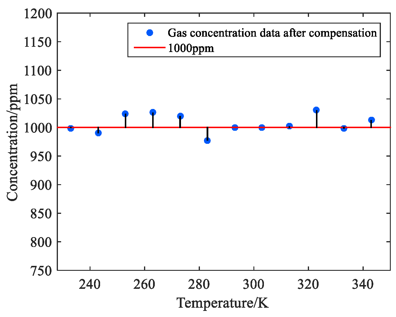
| Temperature/K | Measured Value/ppm | Relative Error/% | Compensated Concentration/ppm | Error /ppm | Relative Error /% |
|---|---|---|---|---|---|
| 233 | 1062 | 6.2 | 999 | −1 | −0.1 |
| 243 | 1048 | 4.8 | 990 | −10 | −1.0 |
| 253 | 1076 | 7.6 | 1024 | 24 | 2.4 |
| 263 | 1069 | 6.9 | 1026 | 26 | 2.6 |
| 273 | 1051 | 5.1 | 1020 | 20 | 2.0 |
| 283 | 993 | −0.7 | 977 | −23 | −2.3 |
| 293 | 1000 | 0.0 | 1000 | 0 | 0.0 |
| 303 | 981 | −1.9 | 1000 | 0 | 0.0 |
| 313 | 963 | −3.7 | 1002 | 2 | 0.2 |
| 323 | 966 | −3.4 | 1030 | 30 | 3.0 |
| 333 | 911 | −8.9 | 998 | −2 | −0.2 |
| 343 | 897 | −10.3 | 1013 | 13 | 1.3 |
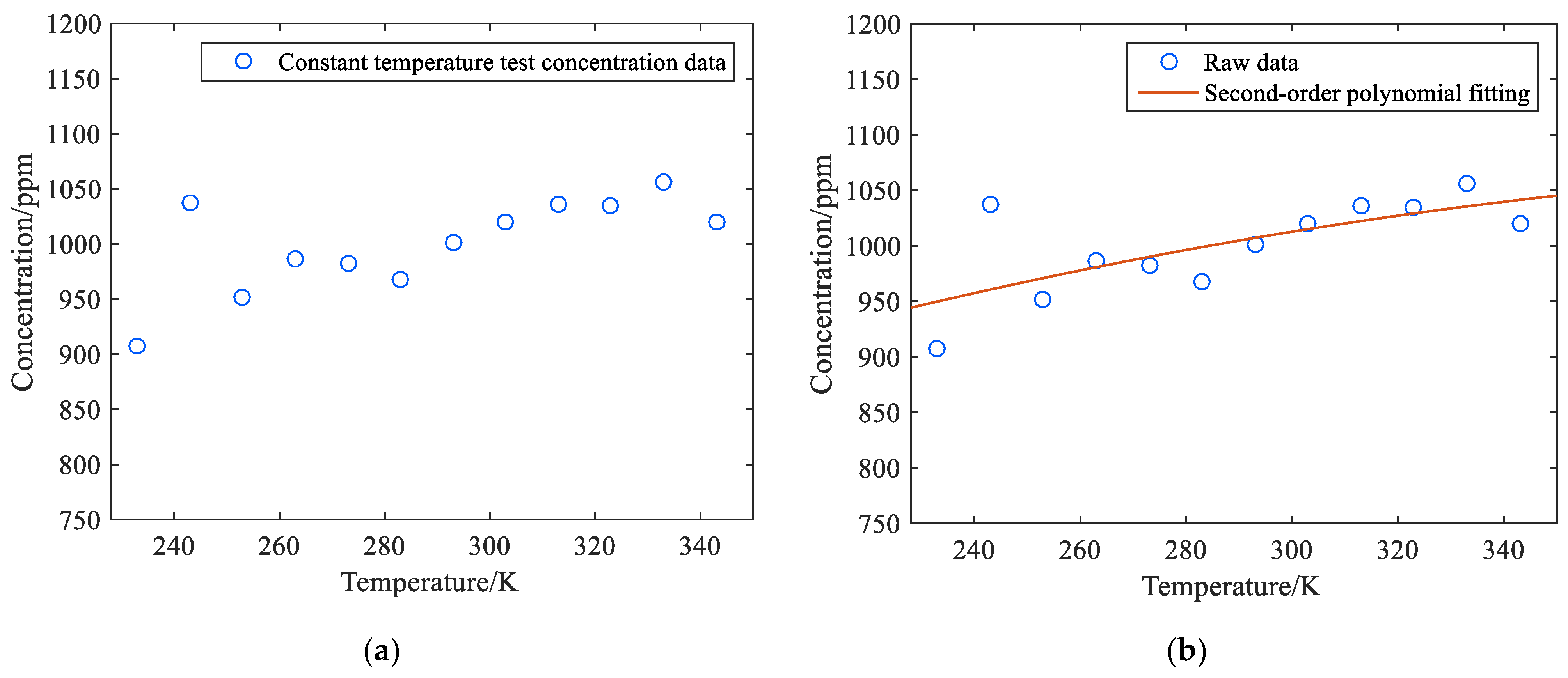
| Temperature/K | Gas Concentration/ppm | Error/ppm | Relative Error/% |
|---|---|---|---|
| 233 | 908 | −92 | −9.2 |
| 243 | 1037 | 37 | 3.7 |
| 253 | 952 | −48 | −4.8 |
| 263 | 986 | −14 | −1.4 |
| 273 | 982 | −18 | −1.8 |
| 283 | 968 | −32 | −3.2 |
| 293 | 1001 | 1 | 0.1 |
| 303 | 1020 | 20 | 2.0 |
| 313 | 1036 | 36 | 3.6 |
| 323 | 1035 | 35 | 3.5 |
| 333 | 1056 | 56 | 5.6 |
| 343 | 1020 | 20 | 2.0 |
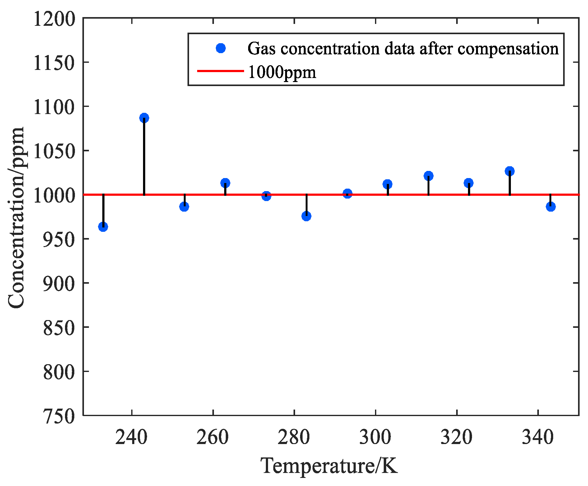
| Temperature/K | Measured Value/ppm | Relative Error/% | Compensated Concentration/ppm | Error /ppm | Relative Error /% |
|---|---|---|---|---|---|
| 233 | 908 | −9.2 | 963 | −37 | −3.7 |
| 243 | 1037 | 3.7 | 1087 | 87 | 8.7 |
| 253 | 952 | −4.8 | 987 | −13 | −1.3 |
| 263 | 986 | −1.4 | 1013 | 13 | 1.3 |
| 273 | 982 | −1.8 | 998 | −2 | −0.2 |
| 283 | 968 | −3.2 | 976 | −24 | −2.4 |
| 293 | 1001 | 0.1 | 1001 | 1 | 0.1 |
| 303 | 1020 | 2.0 | 1012 | 12 | 1.2 |
| 313 | 1036 | 3.6 | 1021 | 21 | 2.1 |
| 323 | 1035 | 3.5 | 1013 | 13 | 1.3 |
| 333 | 1056 | 5.6 | 1027 | 27 | 2.7 |
| 343 | 1020 | 2.0 | 987 | −13 | −1.3 |
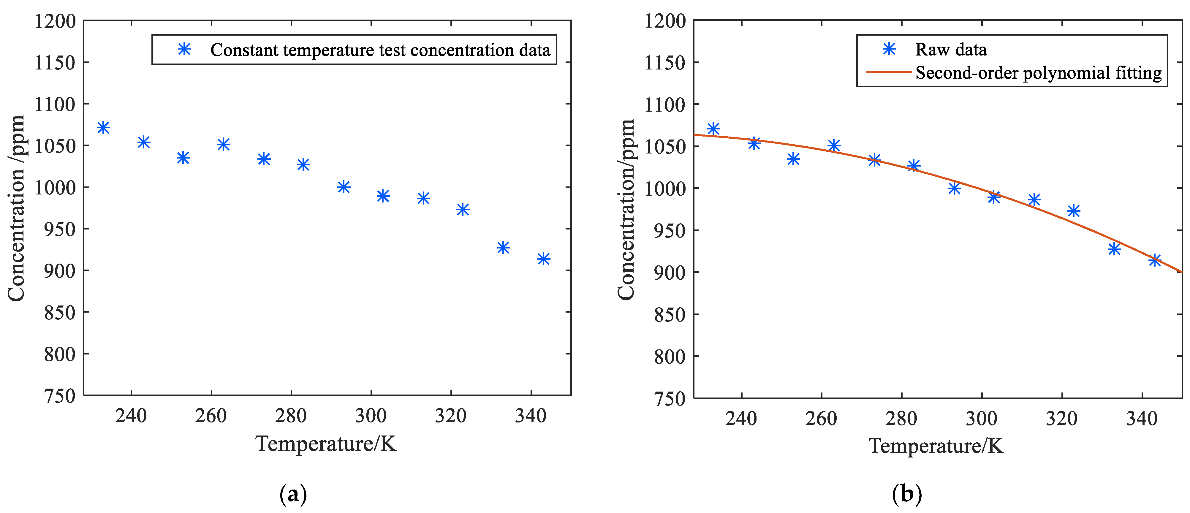
| Temperature/K | Gas Concentration/ppm | Error/ppm | Relative Error/% |
|---|---|---|---|
| 233 | 1071 | 71 | 7.1 |
| 243 | 1054 | 54 | 5.4 |
| 253 | 1035 | 35 | 3.5 |
| 263 | 1051 | 51 | 5.1 |
| 273 | 1033 | 33 | 3.3 |
| 283 | 1027 | 27 | 2.7 |
| 293 | 1000 | 0 | 0.0 |
| 303 | 989 | −11 | −1.1 |
| 313 | 986 | −14 | −1.4 |
| 323 | 973 | −27 | −2.7 |
| 333 | 927 | −73 | −7.3 |
| 343 | 914 | −86 | −8.6 |
| Temperature/K | Measured Value/ppm | Relative Error/% | Compensated Concentration/ppm | Error /ppm | Relative Error /% |
|---|---|---|---|---|---|
| 233 | 949 | −5.10 | 1016 | 16 | 1.6 |
| 243 | 1047 | 4.75 | 1004 | 4 | 0.4 |
| 253 | 857 | −14.32 | 992 | −8 | −0.8 |
| 263 | 866 | −13.44 | 1015 | 15 | 1.5 |
| 273 | 824 | −17.57 | 1008 | 8 | 0.8 |
| 283 | 868 | −13.18 | 1013 | 13 | 1.3 |
| 293 | 1000 | 0.00 | 1000 | 0 | 0.0 |
| 303 | 985 | −1.49 | 1004 | 4 | 0.4 |
| 313 | 938 | −6.15 | 1019 | 19 | 1.9 |
| 323 | 931 | −6.94 | 1025 | 25 | 2.5 |
| 333 | 913 | −8.70 | 998 | −2 | −0.2 |
| 343 | 906 | −9.40 | 1008 | 8 | 0.8 |
Disclaimer/Publisher’s Note: The statements, opinions and data contained in all publications are solely those of the individual author(s) and contributor(s) and not of MDPI and/or the editor(s). MDPI and/or the editor(s) disclaim responsibility for any injury to people or property resulting from any ideas, methods, instructions or products referred to in the content. |
© 2023 by the authors. Licensee MDPI, Basel, Switzerland. This article is an open access article distributed under the terms and conditions of the Creative Commons Attribution (CC BY) license (https://creativecommons.org/licenses/by/4.0/).
Share and Cite
Wang, Y.; Wang, X. Temperature Compensation Algorithm of Air Quality Monitoring Equipment Based on TDLAS. Mathematics 2023, 11, 2656. https://doi.org/10.3390/math11122656
Wang Y, Wang X. Temperature Compensation Algorithm of Air Quality Monitoring Equipment Based on TDLAS. Mathematics. 2023; 11(12):2656. https://doi.org/10.3390/math11122656
Chicago/Turabian StyleWang, Yue, and Xiaoli Wang. 2023. "Temperature Compensation Algorithm of Air Quality Monitoring Equipment Based on TDLAS" Mathematics 11, no. 12: 2656. https://doi.org/10.3390/math11122656
APA StyleWang, Y., & Wang, X. (2023). Temperature Compensation Algorithm of Air Quality Monitoring Equipment Based on TDLAS. Mathematics, 11(12), 2656. https://doi.org/10.3390/math11122656