A Model for a Vacation Queuing Policy Considering Server’s Deterioration and Recovery

Abstract

In this paper, we present a vacation queue model in which the service rate of the server deteriorates during the service period (e.g., due to the fatigue of a human server or the wear and ageing of machinery) and recovers during the vacation period (e.g., following a recuperation period for a human sever or the servicing of a machine). During the recuperation period, the main server is replaced with a temporary server with inferior capabilities. Using the multi-dimensional Markov process, we analyze the effects of different vacation policies on the target function and focus on the scheduling of the vacation period as a function of the deterioration and recovery rates. It is shown that the use of vacations to allow the server to rest and regain efficiency has a strong and valuable effect on the mean customer waiting time, to the extent that switching servers may be beneficial for the system, even when implemented at a point in time when the main server’s service rate is still much higher than that of the temporary server.

1. Introduction

In a conventional vacation queue, the servers (human or machine) suspend their service duties and leave for a vacation for a given amount of time before returning to service. There are various reasons for the server’s vacation, one of which is the deterioration of the service rate. In some systems, the decision on the vacation is instantaneous (e.g., due to unexpected human sickness or machine failure), while in other systems, the vacation is pre-planned based on the system policies (e.g., labor regulations for a human server or the technical maintenance of a mechanical server). Vacation queueing models can be applied to a large variety of real-world stochastic systems and have therefore attracted interest from many researchers. The idea of vacation queuing was introduced by Levy and Yechiali [1]; in this model, during the idle time of a server in an M/G/1 queue, the server performs a secondary task. The duration of time that the server spends on the secondary task is considered to be a random variable with a known distribution function. Levy and Yechiali [1] proposed two vacation queue models. In the first model, the server, upon returning to the initial queue, stays in the system even if there are no customers, and waits for the next arrival (single vacation policy). In the second model, the server takes another vacation if no customers are in the system at the time of returning to the initial queue (multiple vacations policy). In more recent surveys, Refs. [2,3] discussed additional types of models for vacation queueing systems, each with a different service policy. According to an exhaustive service policy, the server returns from vacation after a random duration and starts to serve customers until becoming idle again (and leaving for the next vacation period). According to the gated service policy, only customers who arrive during the vacation are served upon the server’s return from a vacation, and the server leaves for another vacation after serving only these customers. In the limited-service policy, the server serves a predefined number of customers and leaves for a vacation after serving that number. If the queue is empty upon the return to service, the server waits for the first customer to arrive and continues according to the limited queue policy. Ibe and Isijola [4] considered a system with two vacation types. One type of vacation follows a busy service period, while the other type follows a relaxed service period in which the server is idle for part of the time. This model is based on human as well as technical behaviors. It considers the case of human servers, where the server requires a longer recuperation period after an exhaustive service period compared with a more relaxed service period in which the customer arrival rate is relatively low. In the case of a technical server (e.g., a manufacturing CNC machine or an automatic packaging machine), the service time after exhaustive use is likely to be longer than that after limited use or none at all due to the more significant wear and tear of the machine. For further discussion on vacation queues, see, e.g., [5,6,7,8].

Traditionally (as introduced by Levi and Yechiali [1]), the server’s vacation time is used for performing ancillary duties while the main service is suspended. Thus, vacation policies do not improve the main queueing system’s efficiency and may even impair it. In particular, the need to wait for a server to complete ancillary duties may increase customers’ waiting times. According to the extensive research conducted by Polas et al. [9], waiting time has a significant and implicit impact on customer satisfaction (see also [10,11,12]). Hanukov et al. [13] suggested an alternative approach (instead of vacations) for the utilization of a server’s idle time, which can improve the main queueing system’s efficiency. On one hand, all these papers presume that an idle server reduces the overall efficiency of the system. On the other hand, many researchers have pointed out that the effectiveness of non-stop work diminishes over time, while it increases after a rest period. In his book, Pang [14] claimed that, in the context of human servers, “rest is an essential component of working well and working smart” and outlined several studies demonstrating that rest not only enables physical recuperation and the opportunity to think and innovate, but also increases overall productivity. Similarly, Weber et al. [15] stated that “When individuals undertake too many tasks, they actually are less efficient. It has been scientifically proven that idle time is required for developing creativity”. The effect of extended non-stop working hours on the performance of resident physicians in hospitals has been analyzed [16], and as a result, the actual working period of resident physicians between rest periods has been reduced. Another study on the effects of driving time and rest time on the performance of commercial bus and truck drivers concluded that a 15 min recuperation period, following a 2 h continuous driving task, allowed drivers to maintain a safe driving performance [17].

Likewise, a machine might process a task at a much slower rate because of wear and tear, thus needing time to be serviced or repaired. To this end, the authors of [18] considered maintenance control models in which the deterioration of the performance of a machine is modeled as a discrete-time Markov chain. At each state transition in the chain, the machine is either left untouched for the next service or it is repaired/replaced with another machine. If the machine is repaired, service is suspended during the repair period, while if the machine is replaced, services continue with the replacement machine.

To the best of our knowledge, Eisen [19] was the first to introduce the term “deteriorating server”. In his model, the mean service time increases after each customer is served, but due to the complexity of the problem, he focused on simple cases where the number of states is relatively small (e.g., three levels of service rates: normal, slow, and down) in order to obtain an analytical solution. For larger problems, Eisen proposed using simplified ergodic Markovian tools and selected arbitrary constants. In a more recent study, Kaufman and Lewis [20] considered a production machine maintenance policy modeled on a single-server queue. The machine is subject to deterioration that results in slower service rates and, eventually, in failure. They proposed a maintenance policy that considers the state of the machine (server) and the number of customers (jobs) in the queue. They also presented a repair model in which the costs of the server are fixed and a replacement model in which variable costs are considered. They showed that in general, the optimal maintenance policies have a switching curve structure that is monotonous in the server state. Yang et al. [21] considered maintenance in an M/M/1 queue which is subject to random shocks that cause a sharp deterioration of the service rate, and they proposed a preventative maintenance policy. Fitouhi and Nourelfath [22] addressed the problem of integrating noncyclical preventive maintenance and tactical production planning for a single machine. Given a set of products that must be produced in lots during a specified finite planning horizon, the maintenance policy suggests possible preventive replacements at the beginning of each production planning period to achieve minimal repairs and machine failures. In a recent study conducted by Huang et al. [23], the authors considered two types of queues, with each queue characterized by different exponential service requirements and serviced by a single server with a deteriorating service rate. In each state, the server can choose which queue to serve or to undergo a maintenance procedure. There are costs associated with waiting customers and with the cost of maintenance (the problem is derived from the semi-conductor manufacturing industry). The authors showed that a fixed maintenance policy is optimal for general arrival and server state processes, and a joint scheduling and maintenance policy is optimal when the maintenance policy is independent of the queue lengths, using a semi-Markov decision process (SMDP) model. Bouslah et al. [24] addressed the problem of maintenance control for production lines, where the reliability of each machine depends on the prevention of failures in other machines. As an illustration of this problem, they studied a two-machine line model. Choudhary et al. [25] also considered the deterioration of the server’s efficiency during service, which was recovered through a vacation of a random time duration. For clarification, Table 1 summarizes previous studies that address the deterioration of the server.

Table 1. Summary of studies on deteriorating service rates.

	Prop1	Prop2	Prop3	Prop4	Prop5	Prop6	Prop7	Prop8	Prop9	Comments
Our paper	√	√	√	√	√	√	√	√	√
Eisen (1963) [19]										a, d
Kaufman & Lewis (2007) [20]	√	√	√							b, d
Yang et al. (2009) [21]	√	√	√							b, d
Fitouhi & Nourelfath (2012) [22]	√		√							c, d
Huang et al. (2018) [23]	√	√	√							b, d
Bouslah et al. (2018) [24]		√	√							b, d
Choudhary et al. (2021) [25]	√	√	√	√						d

Prop1: Vacation model. Prop2: Considers server’s efficiency deterioration during the work period. Prop3: Utilizing the vacation as a tool for efficiency recovery. Prop4: The deterioration depending on the amount of work already done in the cycle. Prop5: The recovery depending on the vacation mean time. Prop6: The main server is replaced by the temporary server during the vacation. Prop7: Setting optimal number of services in each cycle. Prop8: Setting optimal mean vacation time. Prop9: Comparison with a non-stop working model. a: The server’s efficiency randomly changes up and down, independently of the amount of work done. b: The server’s efficiency randomly deteriorates, independently of the amount of work done. c: The vacation diminishes the probability of failure. d: The vacation initiates the server’s state, independently of the vacation duration.

An additional stream of research that is related to our work is the so-called ‘queues with modulated service rate’ (also called ‘queues in a random environment’), according to which the service system operates in different environments, and in each environment, the server serves customers at a different service rate. Examples of such a system include traffic flow control that is affected by scheduled or unscheduled incidents, and computer systems in which the processing rate depends on the applications running in parallel (see, e.g., [26]). The studies in this stream assume that the service rate of a specific service depends on the current environment and is independent of prior services. In contrast to these models, in our work, the current service’s execution is affected by prior services, such that the service rate of the current service depends on the following factors: (i) the number of services that have already been provided by the server in the work period; (ii) the service rates of the previous services provided by the server; and (iii) the time that the server spent in the vacation period before starting the new working period. This model is formulated and used to provide a scheme for determining the optimal allocation of the server’s active (in service) and idle (in vacation) time in order to increase the service system’s efficiency, which is the main goal of our work.

Another possible vacation policy was introduced by Servi and Finn [27], who proposed the ‘working vacation’ scheme, where the server changes the service rate during the vacation period (instead of no service at all, as in the previous models). Bouchentouf et al. [28] extended the working vacation scheme to the M/M/c/N feedback queueing system with breakdowns and customers’ impatience. They developed an optimization problem based on expected cost function. Do et al. [29] considered the M/M/1 retrial queue with strategic customers and working vacation. They investigated the optimal and the Nash equilibrium strategies and compared different scenarios regarding information availability. For further discussion on working vacation models, see, e.g., [30,31,32].

In this paper, we introduce a variation of the conventional vacation queueing policy that takes into account and quantifies the effect of the server’s rest and recuperation on the system’s effectiveness. According to the proposed model, the effectiveness of the server deteriorates during service and is increased during the recuperation period. Accordingly, the main server leaves the service from time to time for recuperation, and is temporarily replaced during the recuperation period by a secondary server (who/which is less effective). The main server returns to service upon the conclusion of the recuperation period. The paper focuses on the time when the main server leaves service and the length of the recuperation period. While Choudhary et al. [25] assumed that the working and vacation durations are exogenous variables that cannot be controlled by the system, in reality the system’s manager can control these variables (e.g., by controlling the vacation duration) in many service systems. Thus, in the current work, we extend this model, taking the working and vacation durations as endogenous variables, and provide a scheme for the system’s manager to optimize the vacation policy.

We consider two types of systems: (i) a system in which the server’s efficiency level deteriorates to 0 after a long time, meaning that departing for a vacation is mandatory; and (ii) a system with a deteriorating service rate that, after a long time, reaches a certain (low) level, meaning that, theoretically, the server can operate for an infinite period of time without vacations. As mentioned above, in a large number of practical situations, the rate of service in a service system may decrease randomly. For example, a human worker (e.g., a cashier at a supermarket checkout, an officer at an airline check-in counter, or a worker on an assembly line) is likely to work slower when s/he is tired; likewise, a machine (e.g., a computer, a manufacturing machine, or an automatic food-packaging machine) might process a task at a much slower rate as a result of wear and tear. Thus, a worker needs time to recuperate, and a machine needs time to be serviced or repaired, during which he/she/it can be replaced with a temporary worker or machine.

Given the proposed queuing system described above, we address the following research questions:

• How many customers should be served before releasing the main server for a vacation?
• How long should the server spend on vacation in each cycle in order to minimize the customers’ mean sojourn time in the system?
• How does utilizing the vacation period to recover the server’s efficiency affect the customer waiting time?

The main contributions of the paper are as follows:

(i)

We constructed a two-stage service system with a proposed vacation policy as a quasi-birth-and-death (QBD) process and developed quantitative performance measures.

(ii)

We developed a methodology for determining the optimal number of customers to be served during the working period and the optimal mean time of the vacation period.

(iii)

We show that the main server’s service rate may be much higher than the temporary server’s rate at the optimal switching point.

(iv)

We show the percentage of improvement achieved using the suggested vacation policy.

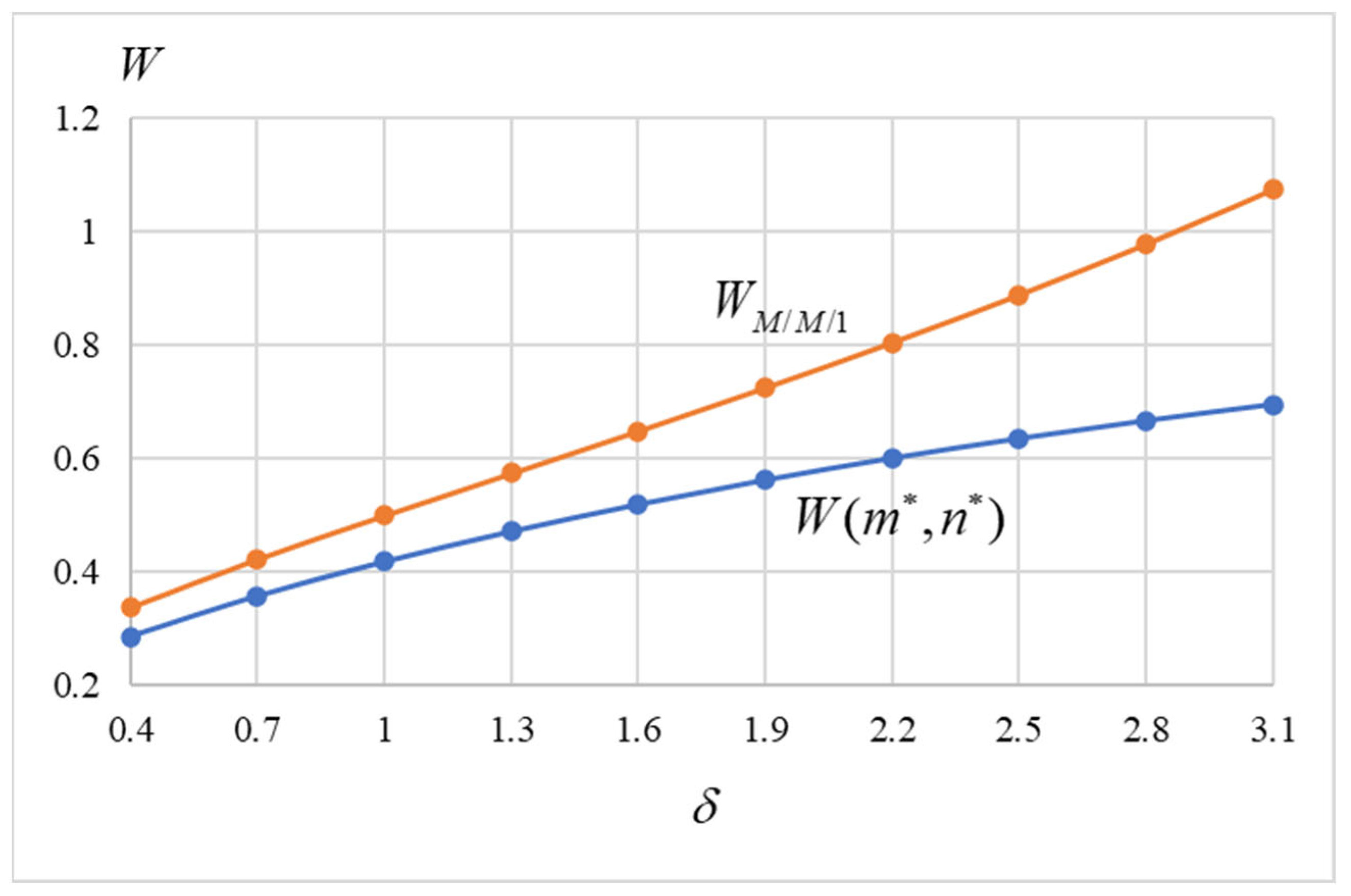
The paper is organized as follows: Section 2 describes the model formulation, and Section 3 provides a general economic analysis using a benchmark system. In Section 4, we compare the performance of the proposed model with that of a regular M/M/1 model with a deteriorating server. Section 5 provides concluding remarks.

Note that, although each of the variables and parameters used in this paper is defined and described when required, a comprehensive detailed list of notations is provided in Appendix A.

2. Model Formulation

Here, we consider a service system with a single server. Customers arrive according to a Poisson process with rate $\lambda$. The server’s efficiency level (hereafter EL) deteriorates after each service is provided. The server provides n services and then leaves for a vacation recovery period, irrespective of the number of customers currently present in the system. The duration of the vacation follows an exponential distribution with rate $\alpha$. During the vacation, the server’s EL increases in time. Let m be the mean EL when the server returns to the system (this can be smaller or larger than 1). Let $Ef{f}_k$, $1\le k\le n+1$, be the server’s mean EL when providing the $k^{th}$ service, where $k=1$ after the server’s return from a vacation and provision of the first service in the current cycle, and $k=n+1$ just before the server leaves for a vacation (the last service in the work period). Let ${\mu }_k=\mu Ef{f}_k$ be the rate of the $k^{th}$ service provided by the server, where μ is the nominal service rate. Accordingly, $Ef{f}_{k+1}<Ef{f}_k$, and so ${\mu }_{k+1}<{\mu }_k$. During the vacation, the main server (hereafter MS) is replaced with a temporary server (hereafter TS). The duration of a service during the vacation period, during which these services are performed by the TS, is exponentially distributed with rate $\beta$. When the MS returns from the vacation, he/she/it joins the system even if there are no customers. If, upon returning from the vacation, the MS finds that the TS is providing a service to a customer, the MS waits inside the system until the service’s completion and then replaces the TS.

The system’s manager aims to use the vacation as a tool for improving efficiency for future customers, which is accomplished at the expense of current customers. Thus, the system’s manager intentionally sets the vacation policy, which involves setting both (i) the number of customers served by the MS in each work period (n) and (ii) the mean vacation time ($1/\alpha$). Such a control structure, in which a decision is made regarding the mean vacation time, is in line with prior works (see, e.g., [33]). Note that $1/\alpha$ can be described by the values n and m (the greater the reduction in the mean EL that needs to be regained during the vacation ($m-Ef{f}_{n+1}$), the longer the required vacation will be). Thus, for a convenient presentation of the analysis, m and n are considered as the system’s decision variables. An example based on the explicit expression of the mean vacation time as a function of n and m is presented in the next section.

In order to analyze the system in a steady state, it is formulated as a quasi-birth-and-death (QBD) process. The system’s state is defined by a two-dimensional vector $(L,S)$. L denotes the number of customers in the system in the steady state, and S denotes the MS’s status in the steady state, as follows: (i) if S is equal to any value between 1 and n, S denotes the step number of the service, which is given by either the number of customers served since the last vacation (when the server is active in the system) or the step number of the next service (when the server is idle in the system and waits for the next customer). (ii) If S equals ‘v’, this indicates that the MS is on vacation; (iii) if S equals 0, this indicates that the MS has just returned from a vacation and is waiting in the system for the completion of the TS’s service. We define the steady-state joint probability distribution function of the two-dimensional Markovian process as $p_{i,j}=\mathrm{Pr}(L=i,S=j)$, $i=0,1,2,\dots$; $j=1,2,\dots n,v,0$.

In order to construct the infinitesimal generator matrix Q of the corresponding QBD process, the system states are arranged in the following order: $\{(0,1),(0,2),\dots ,(0,n),(0,v);(i,1),(i,2),\dots ,(i,n),(i,v),(i,0);\dots \}$, $i=0,1,2,\dots$.

Then,

$$Q=\left(\begin{array}{cccccc}{B}_{1,1}& B_{1,2}& 0& 0& 0& \cdots \\ B_{2,1}& A_1& A_0& 0& 0& \cdots \\ 0& A_2& A_1& A_0& 0& \cdots \\ 0& 0& A_2& A_1& A_0& \\ ⋮& ⋮& & \ddots & \ddots & \ddots \end{array}\right),$$

(1)

where the matrix $B_{1,1}$ is of the order $(n+1)\times (n+1)$, $B_{1,2}$ is of the order $(n+1)\times (n+2)$, $B_{2,1}$ is of the order $(n+2)\times (n+1)$, and $A_0$, $A_1$, and $A_2$, are each of the order $(n+2)\times (n+2)$. These matrices are given as follows: $A_0=\lambda I$, where I is the identity matrix:

$$\begin{gathered} B_{1,1}=\left(\begin{array}{ccccc}-\lambda & 0& \cdots & 0& 0\\ 0& -\lambda & \cdots & 0& 0\\ ⋮& ⋮& \ddots & ⋮& ⋮\\ 0& 0& \cdots & -\lambda & 0\\ \alpha & 0& \cdots & 0& -(\lambda +\alpha )\end{array}\right),B_{1,2}=\left(\begin{array}{ccccc}\lambda & 0& \cdots & 0& 0\\ 0& \lambda & \cdots & 0& 0\\ ⋮& ⋮& \ddots & ⋮& ⋮\\ 0& 0& \cdots & \lambda & 0\end{array}\right), \\ {B}_{2,1}=\left(\begin{array}{ccccc}0& {\mu }_1& 0& \cdots & 0\\ 0& 0& {\mu }_2& \cdots & 0\\ ⋮& ⋮& & \ddots & ⋮\\ 0& 0& 0& \cdots & {\mu }_n\\ 0& 0& 0& \cdots & \beta \\ \beta & 0& 0& \cdots & 0\end{array}\right),A_2=\left(\begin{array}{cccccc}0& {\mu }_1& 0& \cdots & 0& 0\\ 0& 0& {\mu }_2& \cdots & 0& 0\\ ⋮& ⋮& & \ddots & ⋮& ⋮\\ 0& 0& 0& \cdots & {\mu }_n& 0\\ 0& 0& 0& \cdots & \beta & 0\\ \beta & 0& 0& \cdots & 0& 0\end{array}\right), \\ {A}_1=\left(\begin{array}{cccccc}-(\lambda +{\mu }_1)& 0& \cdots & 0& 0& 0\\ 0& -(\lambda +{\mu }_2)& & 0& 0& 0\\ ⋮& ⋮& \ddots & ⋮& ⋮& ⋮\\ 0& 0& & -(\lambda +{\mu }_n)& 0& 0\\ 0& 0& \cdots & 0& -(\lambda +\alpha +\beta )& \alpha \\ 0& 0& \cdots & 0& 0& -(\lambda +\beta )\end{array}\right). \end{gathered}$$

For each system’s level i, we define the corresponding probability vector as ${\overrightarrow{p}}_0\equiv \left(p_{0,1},p_{0,2},\dots ,p_{0,n},p_{0,v}\right)$ and ${\overrightarrow{p}}_i\equiv \left(p_{i,1},p_{i,2},\dots ,p_{i,n},p_{i,v},p_{i,0}\right)$, $i=1,2,3,\dots$. Then, the total probability vector of all the system states is given by $\overrightarrow{p}\equiv ({\overrightarrow{p}}_0,{\overrightarrow{p}}_1,{\overrightarrow{p}}_2,\dots )$. Let $\overrightarrow{e}={(1,1,\dots ,1)}^T$ be a column vector with all its entries being equal to one. The system’s balance equations are given by

$$\overrightarrow{p}Q=\overrightarrow{0},{\displaystyle \sum _{i=0}^{\infty }{\overrightarrow{p}}_i\cdot \overrightarrow{e}}=1.$$

(2)

Theorem 1.

The system’s stability condition is given by

$$\lambda <(n+2){\left[\frac{1}{\alpha }+\frac{1}{\beta }+{\displaystyle \sum _{i=1}^n\frac{1}{{\mu }_i}}\right]}^{-1}$$

(3)

Proof of Theorem 1.

Let

$$A=A_0+A_1+A_2=\left(\begin{array}{cccccc}-{\mu }_1& {\mu }_1& 0& \cdots & 0& 0\\ 0& -{\mu }_2& {\mu }_2& \cdots & 0& 0\\ ⋮& ⋮& & \ddots & ⋮& ⋮\\ 0& 0& 0& \cdots & {\mu }_n& 0\\ 0& 0& 0& \cdots & -\alpha & \alpha \\ \beta & 0& 0& \cdots & 0& -\beta \end{array}\right),$$

and let $\overrightarrow{\pi }=({\pi }_1,{\pi }_2,\dots ,{\pi }_n,{\pi }_v,{\pi }_0)$ be the unique solution of

$$\begin{array}{l}\overrightarrow{\pi }A=\overrightarrow{0},\\ \overrightarrow{\pi }\overrightarrow{e}=1.\end{array}$$

(4)

Then, according to Neuts [34], the condition for stability is given by

$$\overrightarrow{\pi }{A}_0\overrightarrow{e}<\overrightarrow{\pi }{A}_2\overrightarrow{e}.$$

(5)

Solving the set in Equation (4) and substituting $\overrightarrow{\pi }$ in Equation (5) proves the claim. □

Let R be the rate matrix satisfying

$$A_0+R{A}_1+R^2{A}_2=0.$$

(6)

Then, the steady-state probabilities of the queueing system are calculated (see Neuts [34]) by

$${\overrightarrow{p}}_i={\overrightarrow{p}}_1{R}^{i-1},i=1,2,3,\dots ,$$

(7)

where ${\overrightarrow{p}}_0$ and ${\overrightarrow{p}}_1$ are calculated using some of the balance equations along with the normalization equation, specifically by

$$\begin{array}{l}{\overrightarrow{p}}_0{B}_{1,1}+{\overrightarrow{p}}_1{B}_{2,1}=\overrightarrow{0},\\ {\overrightarrow{p}}_0{B}_{1,2}+{\overrightarrow{p}}_1\left[A_1+R{A}_2\right]=\overrightarrow{0},\\ {\overrightarrow{p}}_0+{\overrightarrow{p}}_1{\left[I-R\right]}^{-1}\overrightarrow{e}=1.\end{array}$$

(8)

For a given m and n, let $L(m,n)$ be the mean number of customers in the system, let $L_q(m,n)$ be the mean number of customers in the queue, let $W(m,n)$ be the mean sojourn time of a customer in the system, and let $W_q(m,n)$ be the mean waiting time of a customer in the queue. $L(m,n)$ is given by

$$L(m,n)={\displaystyle \sum _{i=1}^{\infty }i{\overrightarrow{p}}_i\overrightarrow{e}}={\displaystyle \sum _{i=1}^{\infty }i{\overrightarrow{p}}_1{R}^{i-1}\overrightarrow{e}}={\overrightarrow{p}}_1{[I-R]}^{-2}\overrightarrow{e}.$$

(9)

Then, $L_q(m,n)$ is given by

$$L_q(m,n)=L(m,n)-(1-{\overrightarrow{p}}_0\overrightarrow{e}).$$

(10)

According to Little’s law, $W(m,n)=L(m,n)/\lambda$ and $W_q(m,n)=L_q(m,n)/\lambda$.

Let $p_{rep}(m,n)$ be the portion of time for which service is provided by the TS, and let $p_{main}(m,n)$ be the portion of time for which service is provided by the MS. Let ${\overrightarrow{u}}_1={(0,0,0,\dots ,0,1)}^T$ be an $(n+1)$-dimensional column vector and let ${\overrightarrow{u}}_2={(0,0,0,\dots ,0,1,1)}^T$ be an $(n+2)$-dimensional column vector. Then, $p_{rep}(m,n)$ is given by

$$p_{rep}(m,n)={\overrightarrow{p}}_0{\overrightarrow{u}}_1+{\displaystyle \sum _{i=1}^{\infty }{\overrightarrow{p}}_i{\overrightarrow{u}}_2}={\overrightarrow{p}}_0{\overrightarrow{u}}_1+{\displaystyle \sum _{i=1}^{\infty }{\overrightarrow{p}}_1{R}^{i-1}{\overrightarrow{u}}_2}={\overrightarrow{p}}_0{\overrightarrow{u}}_1+{\overrightarrow{p}}_1{[I-R]}^{-1}{\overrightarrow{u}}_2,$$

(11)

and consequently, $p_{main}(m,n)=1-p_{rep}(m,n)$. Let $p_{vac}(m,n)$ be the portion of time that the MS is on vacation, and let ${\overrightarrow{u}}_3={(0,0,0,\dots ,0,1,0)}^T$ be an $(n+2)$-dimensional column vector. Then, $p_{vac}(m,n)$ is given by

$$p_{vac}(m,n)={\overrightarrow{p}}_0{\overrightarrow{u}}_1+{\displaystyle \sum _{i=1}^{\infty }{\overrightarrow{p}}_i{\overrightarrow{u}}_3}={\overrightarrow{p}}_0{\overrightarrow{u}}_1+{\displaystyle \sum _{i=1}^{\infty }{\overrightarrow{p}}_1{R}^{i-1}{\overrightarrow{u}}_3}={\overrightarrow{p}}_0{\overrightarrow{u}}_1+{\overrightarrow{p}}_1{[I-R]}^{-1}{\overrightarrow{u}}_3.$$

(12)

Let $p_{ava}(m,n)$ be the portion of time that the MS is available in the system after returning from vacation but is waiting for the TS to complete the current service, and let ${\overrightarrow{u}}_4={(0,0,0,\dots ,0,0,1)}^T$ be an $(n+2)$-dimensional column vector. Then, $p_{ava}(m,n)$ is given by

$$p_{ava}(m,n)={\displaystyle \sum _{i=1}^{\infty }{\overrightarrow{p}}_i{\overrightarrow{u}}_4}={\displaystyle \sum _{i=1}^{\infty }{\overrightarrow{p}}_1{R}^{i-1}{\overrightarrow{u}}_4}={\overrightarrow{p}}_1{[I-R]}^{-1}{\overrightarrow{u}}_4,$$

(13)

and consequently, $p_{rep}(m,n)=p_{vac}(m,n)+p_{ava}(m,n)$.

3. Economic Analysis

In this section, we provide a numerical study demonstrating how to determine the optimal values of n, the number of services in each cycle before the MS leaves for a vacation, and m, the mean EL of the MS at the point of returning to the system. We define $Ef{f}_k(t)$, the server’s EL, as a decreasing function of time t, which deteriorates during the $k^{th}$ service. In line with [35], we assume the following exponential structure of $Ef{f}_k(t)$, implying a diminishing marginal return of the server’s EL deterioration during the service:

$$Ef{f}_{k+1}(t)=Ef{f}_k{e}^{-\delta t},k=1,2,\dots ,n,$$

(14)

where $\delta$ is the deterioration rate. According to Equation (14), $Ef{f}_{k+1}(0)=Ef{f}_k$ and $Ef{f}_{k+1}(t)\underset{\hspace{1em}t\to \infty \hspace{1em}}{\to }0$. Due to the exponentiality assumption of the service rate, the deterioration of the efficiency does not affect the service rate during a specific service episode, i.e., the service rate of a particular service is constant during the actual provision of service to a specific customer, which is determined by the EL at the beginning of the service. After a service is completed, the EL for the next customer is updated according to Equation (14). Since the $k^{th}$ service is exponentially distributed with the rate ${\mu }_k$, the $Ef{f}_{k+1}$ is recursively given by

$$Ef{f}_{k+1}={\displaystyle \underset{0}{\overset{\infty }{\int }}Ef{f}_k{e}^{-\delta t}{\mu }_k{e}^{-{\mu }_{k}t}dt}=Ef{f}_k\frac{{\mu }_k}{\delta +{\mu }_k},k=1,2,\dots ,n.$$

(15)

Then, ${\mu }_k$ is recursively given by

$${\mu }_{k+1}=\frac{{\mu }_k^2}{\delta +{\mu }_k},k=1,2,\dots ,n,$$

(16)

where ${\mu }_1=\mu Ef{f}_1=\mu m$ is the maximal service rate in a cycle (which is the service rate of the first customer after the main server returns from the vacation), and ${\mu }_n=\mu Ef{f}_n$ is the minimal service rate in a cycle (which is the service rate for the last customer in the cycle before the main server leaves for a vacation). Thus, the main server leaves for a vacation with a mean EL equal to $Ef{f}_{n+1}.$ According to Equation (16), (i) ${\mu }_k$ monotonically deteriorates with k, and (ii) the service rate approaches zero when the number of services in the cycle approaches infinity, ${\mu }_k\underset{\hspace{1em}k\to \infty \hspace{1em}}{\to }0$. We prove the latter property in the following proposition.

Proposition 1.

The service rate (given in Equation (16)) approaches zero when the number of services in the cycle approaches infinity, ${\mu }_k\underset{\hspace{1em}k\to \infty \hspace{1em}}{\to }0$.

Proof of Proposition 1.

Denote the limit as c. Then,

$c=\underset{k\to \infty }{\lim }{\mu }_k=\underset{k\to \infty }{\lim }{\mu }_{k+1}=\underset{k\to \infty }{\lim }\frac{{\mu }_k^2}{\delta +{\mu }_k}=\frac{\underset{k\to \infty }{\lim }{\mu }_k^2}{\delta +\underset{k\to \infty }{\lim }{\mu }_k}=\frac{c^2}{\delta +c}$. Solving $c=\frac{c^2}{\delta +c}$ leads to $c=0$. □

As mentioned, while on a vacation, the main server recovers according to a time-dependent recovery function, and therefore the EL grows. The main server’s mean EL upon returning to the system, m, depends on the mean EL at the beginning of the vacation $(Ef{f}_{n+1})$ and the mean time spent on vacation $({\alpha }^{-1})$. We assume that m is given by the following function:

$$m=Ef{f}_{n+1}+(m_{\max }-Ef{f}_{n+1})\frac{b}{\alpha +b}.$$

(17)

This function is used because (i) $m\underset{\hspace{1em}\alpha \to \infty \hspace{1em}}{\to }Ef{f}_{n+1}$, i.e., if the server does not take a vacation, the mean EL remains as $Ef{f}_{n+1}$, and (ii) $m\underset{\hspace{1em}\alpha \to 0\hspace{1em}}{\to }{m}_{\max }$, i.e., m approaches a certain constant efficiency value, $m_{\max }$, when the mean duration of the vacation is sufficiently long. As described in the previous section, initially, the system’s manager decides on the number of customers served in each work period (n) and the mean vacation time $(1/\alpha )$. Then, m can be calculated as a function of n and $\alpha$, as given in Equation (17). However, for convenient presentation of the analysis, we consider m and n as the system’s decision variables and then calculate $\alpha$ as a function of m and n. Accordingly, by isolating $\alpha$ in Equation (17), we obtain

$$\alpha =\frac{b(m_{\max }-m)}{m-Ef{f}_{n+1}}.$$

(18)

Let $\alpha (m,n)$ be the return rate from the vacation as a function of m and n, and let ${\mu }_k(m,n)$ be the service rate of the $k^{th}$ service as a function of m and n, where m and n, as mentioned above, are the system’s decision variables.

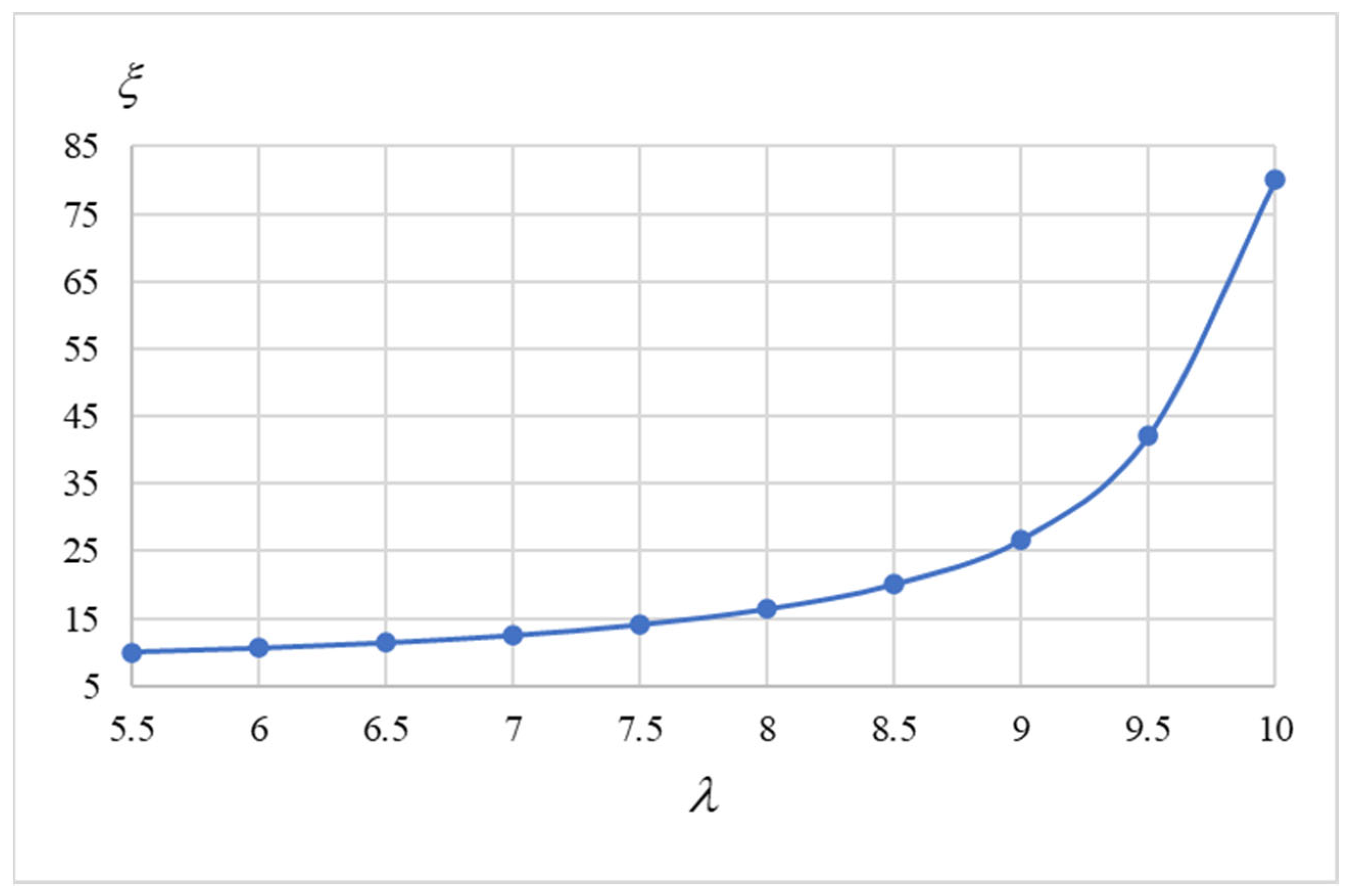
We use the following parameter values for a base illustrative example: Consider a service system in which customers arrive with a rate $\lambda =8[\frac{\mathrm{customers}}{\mathrm{hour}}]$. For the service rates, we set $\mu =30[\frac{\mathrm{customers}}{\mathrm{hour}}]$, which allows us to calculate the MS’s service rate for each service $({\mu }_k),$ and we use $\beta =5[\frac{\mathrm{customers}}{\mathrm{hour}}]$ to represent the TS’s service rate. During the MS’s active period, the EL deteriorates at a rate of $\delta =1$ (see Equation (16)), and during the vacation, the EL grows at a rate of $b=5$ (see Equation (17)). Finally, we set the maximal EL to $m_{\max }=1.8$. These values are used because they satisfy the stability condition, which is given in Theorem 1 for a large range of m and n values, therefore enabling us to analyze the system’s performance for a wide range of parameters. 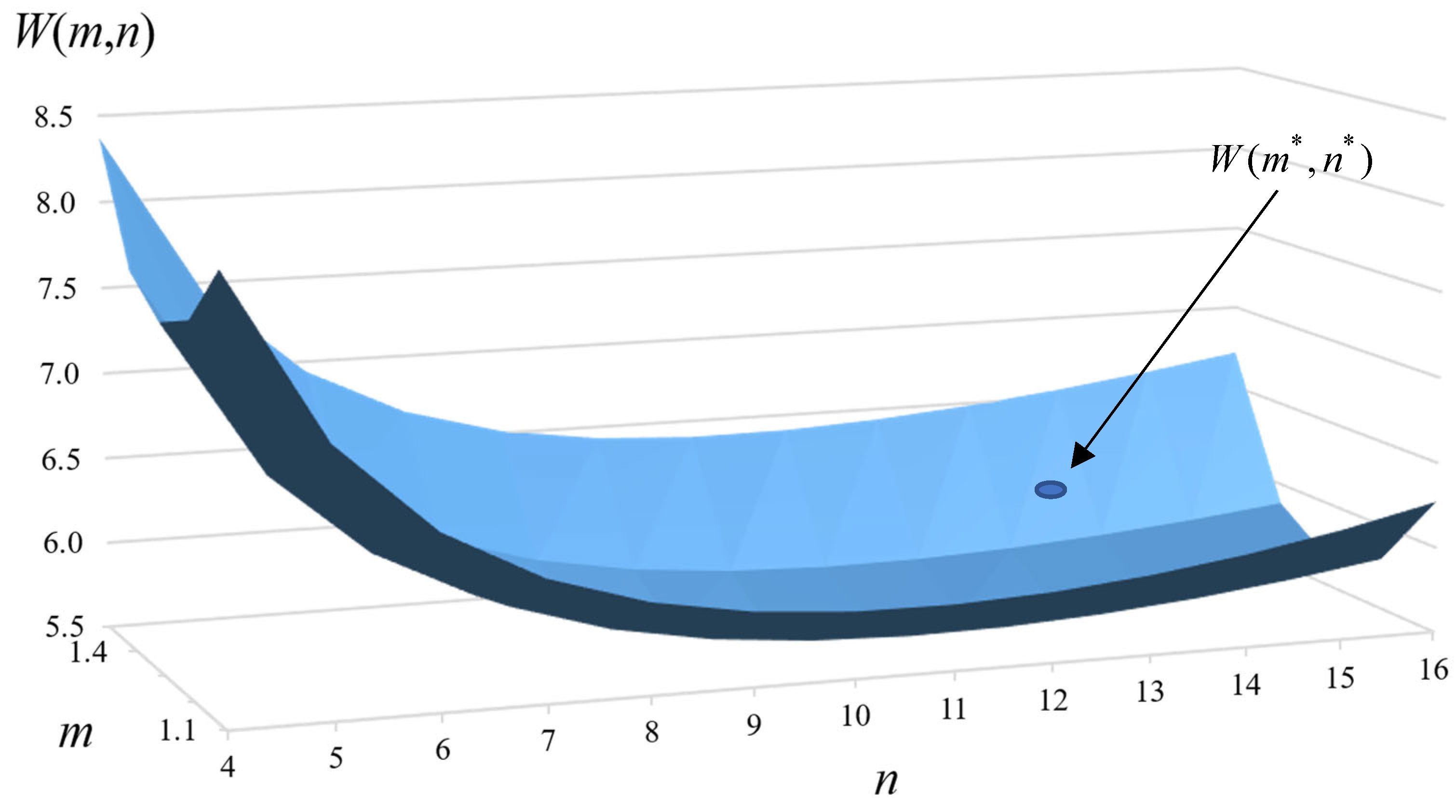Figure 1 and Table 2 present the values of the customers’ mean sojourn time, $W(m,n)$, for a wide range of combinations of $m=\{0.7,0.8,\dots ,1.7\}$ with $n=\{1,2,3,\dots ,20\}$, where the best value (i.e., the minimal value) of $W(m,n)$, denoted as $W(m^{*},n^{*})$, is underlined and printed in bold in Table 2. The values in Table 2 are obtained by substituting the corresponding values of m and n into $W(m,n)=L(m,n)/\lambda$, where $L(m,n)$ is calculated using Equation (9). According to the best solution, the main server serves $n=11$ customers in each cycle and then leaves for a vacation. The main server returns from vacation when their/its mean EL reaches $m=1.3$. Thus, in the optimal setup, according to Equation (18), the server is on vacation for ${\alpha }^{-1}=8.548$ min, and the customers’ mean sojourn time in the system is $W(m,n)=5.479$ min.

Figure 1. Customers’ sojourn time as a function of m and n.

Table 2. Customers’ sojourn time (in minutes) for various values of m and n.

n\m	0.7	0.8	0.9	1	1.1	1.2	1.3	1.4	1.5	1.6	1.7
1	356.939	222.275	162.293	130.409	111.673	100.293	93.909	91.982	96.070	114.678	237.693
2	30.728	24.491	20.808	18.455	16.925	15.993	15.582	15.754	16.806	19.853	32.725
3	17.757	14.374	12.319	10.995	10.144	9.646	9.469	9.661	10.431	12.534	21.072
4	14.007	11.323	9.699	8.660	7.999	7.623	7.508	7.697	8.374	10.202	17.691
5	12.439	9.996	8.534	7.608	7.024	6.697	6.607	6.796	7.437	9.175	16.406
6	11.726	9.341	7.935	7.053	6.502	6.198	6.120	6.310	6.943	8.668	15.952
7	11.451	9.022	7.615	6.743	6.202	5.907	5.835	6.029	6.666	8.417	15.907
8	11.453	8.902	7.456	6.571	6.027	5.732	5.662	5.861	6.512	8.310	16.092
9	11.663	8.919	7.402	6.487	5.930	5.630	5.559	5.763	6.432	8.293	16.417
10	12.058	9.044	7.425	6.465	5.886	5.576	5.502	5.712	6.401	8.333	16.836
11	12.642	9.263	7.511	6.491	5.882	5.557	5.479	5.693	6.406	8.415	17.318
12	13.444	9.577	7.653	6.556	5.910	5.566	5.480	5.699	6.436	8.525	17.845
13	14.519	9.992	7.848	6.657	5.964	5.597	5.502	5.724	6.485	8.658	18.406
14	15.965	10.524	8.100	6.792	6.043	5.647	5.540	5.764	6.549	8.808	18.993
15	17.946	11.201	8.414	6.962	6.145	5.714	5.592	5.817	6.626	8.971	19.600
16	20.762	12.064	8.802	7.170	6.270	5.798	5.657	5.882	6.714	9.146	20.223
17	25.000	13.179	9.277	7.420	6.419	5.899	5.735	5.956	6.811	9.330	20.860
18	31.996	14.650	9.864	7.719	6.596	6.016	5.825	6.041	6.917	9.523	21.508
19	45.553	16.651	10.594	8.077	6.803	6.152	5.928	6.135	7.031	9.723	22.166
20	81.967	19.493	11.517	8.508	7.045	6.309	6.044	6.239	7.152	9.930	22.833

As mentioned above, Figure 1 depicts the value of the sojourn time $W(m,n)$ for various m and n values. As shown here, $W(m,n)$ is a smooth convex function with a minimum value at $m^{*}=1.3$ (approximately 72% of the maximal value of 1.8) for a wide range of values of n. The gradient of $W(m,n)$ remains relatively small for small variations in $m^{*}$ $(m=1.1÷1.5)$ of approximately ±11%, but it is more sensitive to variations in $n^{*}$ in the extreme region $(n<4)$. An interesting observation based on this analysis is that the duration of the vacation period (expressed by m) has a stronger effect on the mean sojourn time of customers in the system than the number of services before the time of leaving for a vacation $(n)$.

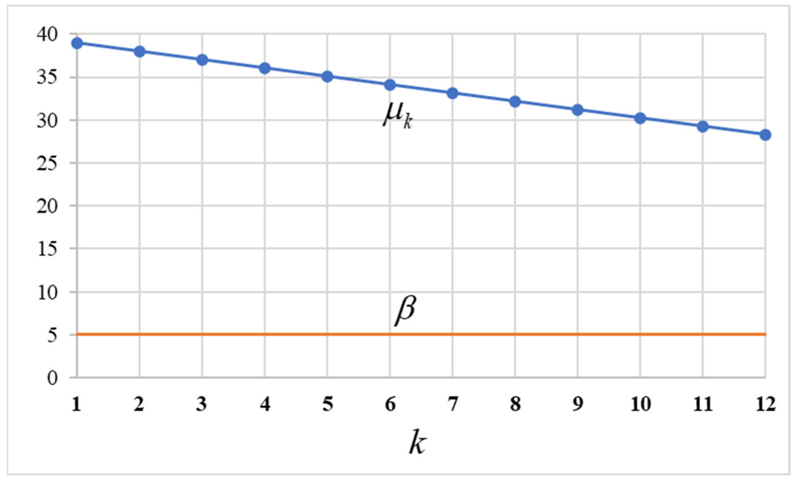
Figure 2 shows how the MS’s service rate deteriorates during the operating time, compared with the constant service rate of the TS. Note that when the servers are switched (i.e., when $k=12$), the MS’s service rate is still much higher than that of the TS (28 vs. 5). This result indicates that switching servers is beneficial for the system, even at the expense of a significant temporary reduction in the current service rate due to the TS’s inferior performance. Intuitively, the switching point should take place when the MS’s service rate is close to the TS’s service rate or even drops below it. However, as shown in the figure, the ideal switching point is when the MS has considerable ‘spare’ capabilities compared with the TS. This can be explained by the recovery period of the main server during the vacation. Note that, as previously mentioned, the service rate of the MS deteriorates in an exponential manner during the work period. The illusion of a linear behavior in Figure 2 is due to the fact that the figure shows a close-up view of the functions within a narrow window of data. For a wider view, see Appendix B.

Figure 2. The MS’s service rate during the operation time (blue curve) and the TS’s constant service rate (red curve). Values are in $\left[\frac{\mathrm{customers}}{\mathrm{hour}}\right]$.

Sensitivity Analysis

In order to investigate the effects of the system’s parameters on the optimal decisions $m^{*}$ and $n^{*}$ on the optimal sojourn time $W(m^{*},n^{*})$, we use the numerical example given at the beginning of this section as a base case and calculate $m^{*}$, $n^{*}$, and $W(m^{*},n^{*})$ for various values of the system’s parameters ($\beta$, $\delta$, b, and $\lambda$), changing the value of a single parameter each time. The results are presented in Figure 3, Figure 4, Figure 5, Figure 6, Figure 7, Figure 8, Figure 9 and Figure 10. Figure 3 shows the results of $W(m^{*},n^{*})$ for different values of $\beta$ (the service rate of the TS). As expected, the best sojourn time $W(m^{*},n^{*})$ is reduced with the increase in the TS’s service rate $\beta$ (a better temporary server). The effect of $\beta$ on $W(m^{*},n^{*})$ is given by a monotonous exponential function, as its effect becomes smaller when $\beta$ is larger than 15 (50% of the nominal value of $\mu$). Assuming that the cost of the TS is proportional to the service rate value, based on these results, it is sufficient to select a TS with a service rate of 50–60% of the MS’s nominal service rate. 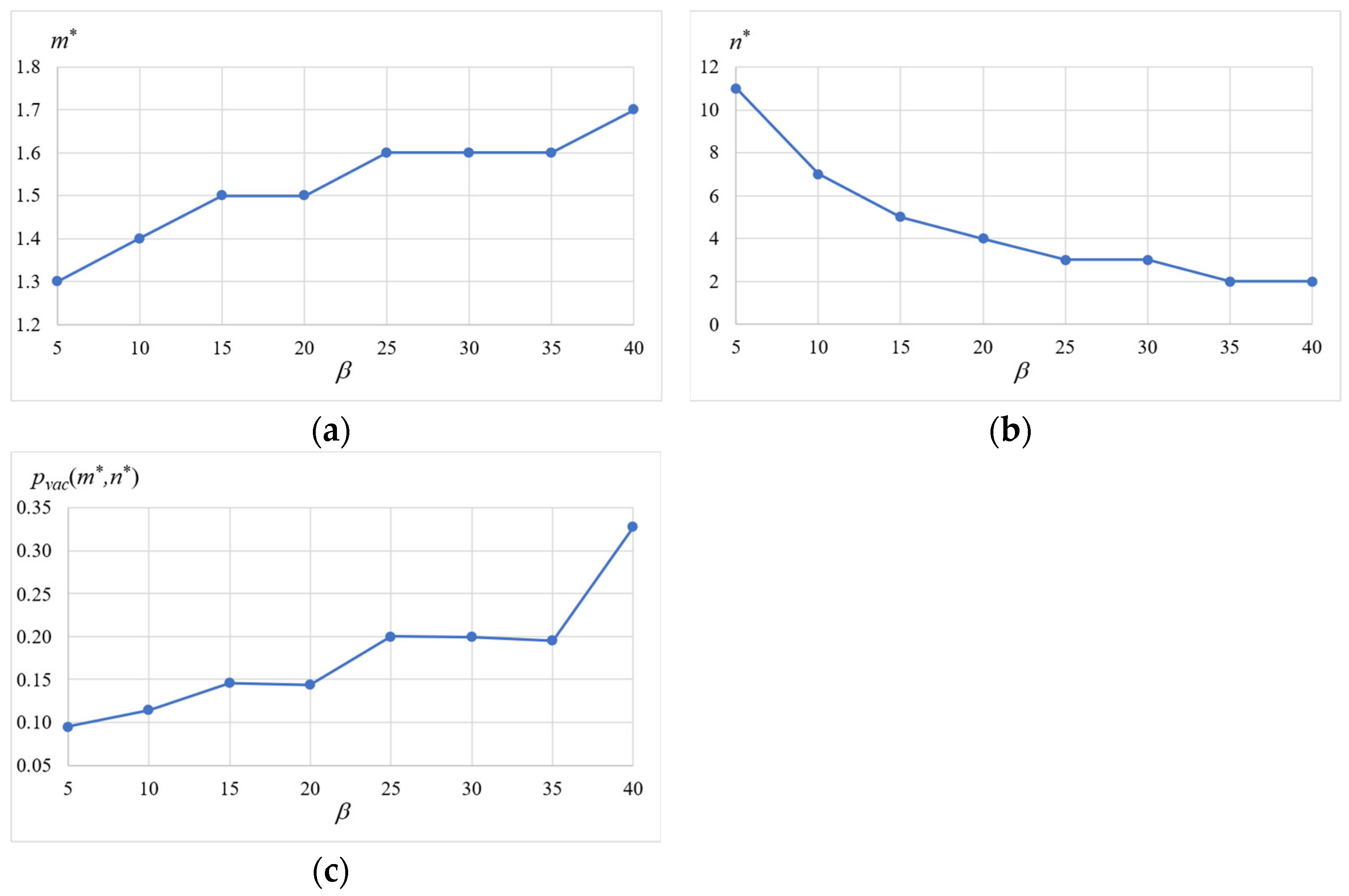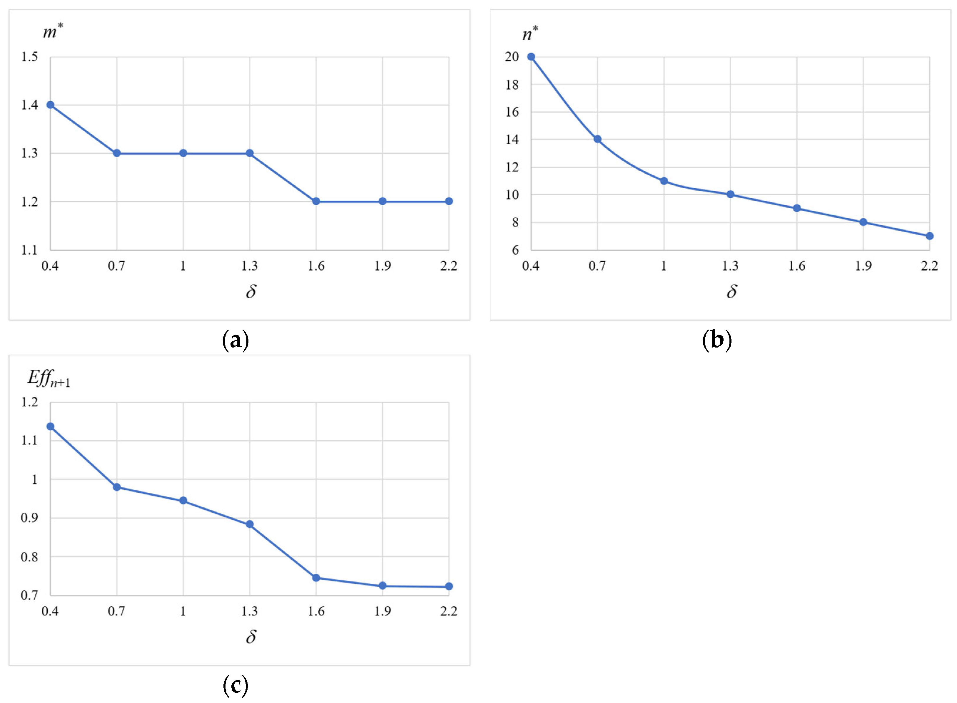Figure 4 shows the simultaneous effects of the TS’s service rate $\beta$ on $m^{*}$, $n^{*}$ and the fraction of time for which the MS is on vacation, $p_{vac}(m^{*},n^{*})$. The conclusions from this figure are as follows: (i) when $\beta$ increases, the optimal number of services provided before leaving for a vacation, $n^{*}$, decreases at an exponential rate, and (ii) the optimal mean EL at the points of the MS’s return, $m^{*}$, increases linearly with $\beta$. Moreover, the figure shows that when $m^{*}$ increases, the $p_{vac}(m^{*},n^{*})$ increases (see, e.g., the switching point from $\beta =35$ to $\beta =40$, where $m^{*}$ increases and $n^{*}$ remains constant). However, interestingly, a decrease in $n^{*}$ does not affect the $p_{vac}(m^{*},n^{*})$ (see, e.g., the switching point from $\beta =30$ to $\beta =35$, where $n^{*}$ decreases and $m^{*}$ remains constant). This result can be explained as follows: if the MS performs fewer services, he/she/it stays in the system for less time; on the other hand, when the MS leaves for a vacation, his/her/its EL is higher and, consequently, the MS needs less time to reach the return level $m^{*}$. Thus, the decrease in $n^{*}$ has two opposite effects on the $p_{vac}(m^{*},n^{*})$, and as a result, the $p_{vac}(m^{*},n^{*})$ does not change. To study this phenomenon in greater depth, Table 3 presents the $p_{vac}(m,n)$ for various values of $m$ and $n$. The table shows that for small values of n ($n=1,2$), an increase in n has a positive effect on the $p_{vac}(m,n)$. However, for larger values of n $(n>7)$, the $p_{vac}(m,n)$ almost remains constant with n. Moreover, Table 3 shows that the $p_{vac}(m,n)$ increases very slightly with n, and then $(n>13)$ decreases very slightly, which can also be explained by the two opposite effects of n on the $p_{vac}(m,n)$, as described above.

Figure 3. $W(m^{*},n^{*})$ for various values of β.

Figure 4. (a) Optimal m, (b) optimal n, and (c) optimal $p_{vac}(m,n)$ for various values of β.

Figure 5. $W(m^{*},n^{*})$ for various values of δ.

Figure 6. (a) Optimal m, (b) optimal n, and (c) optimal $Ef{f}_{n+1}$ for various values of δ.

Figure 7. $W(m^{*},n^{*})$ for various values of b.

Figure 8. (a) Optimal m and (b) optimal n for various values of $b$.

Figure 9. $W(m^{*},n^{*})$ for various values of λ.

Figure 10. (a) Optimal m, (b) optimal n, and (c) optimal $p_{vac}(m,n)$ for various values of λ.

Table 3. Percentage of time for which the MS is on vacation for various values of n and m.

n\m	0.7	0.8	0.9	1	1.1	1.2	1.3	1.4	1.5	1.6	1.7
1	0.0231	0.0265	0.0303	0.0350	0.0408	0.0482	0.0582	0.0723	0.0943	0.1342	0.2322
2	0.0343	0.0388	0.0440	0.0503	0.0580	0.0679	0.0814	0.1007	0.1312	0.1870	0.3238
3	0.0380	0.0427	0.0482	0.0547	0.0629	0.0735	0.0879	0.1087	0.1419	0.2031	0.3547
4	0.0397	0.0445	0.0500	0.0567	0.0651	0.0759	0.0907	0.1123	0.1466	0.2104	0.3693
5	0.0407	0.0455	0.0510	0.0578	0.0663	0.0773	0.0923	0.1142	0.1493	0.2144	0.3774
6	0.0412	0.0460	0.0517	0.0585	0.0670	0.0781	0.0933	0.1154	0.1509	0.2169	0.3824
7	0.0416	0.0464	0.0521	0.0589	0.0675	0.0786	0.0939	0.1163	0.1520	0.2186	0.3856
8	0.0418	0.0467	0.0523	0.0592	0.0678	0.0790	0.0944	0.1168	0.1527	0.2197	0.3878
9	0.0420	0.0468	0.0525	0.0594	0.0680	0.0793	0.0947	0.1172	0.1533	0.2206	0.3893
10	0.0421	0.0469	0.0527	0.0596	0.0682	0.0795	0.0950	0.1175	0.1537	0.2212	0.3904
11	0.0421	0.0470	0.0527	0.0597	0.0683	0.0797	0.0952	0.1178	0.1540	0.2216	0.3913
12	0.0421	0.0470	0.0528	0.0597	0.0684	0.0798	0.0953	0.1180	0.1543	0.2220	0.3919
13	0.0421	0.0470	0.0528	0.0598	0.0685	0.0799	0.0954	0.1181	0.1545	0.2222	0.3923
14	0.0420	0.0470	0.0528	0.0598	0.0685	0.0799	0.0955	0.1182	0.1546	0.2224	0.3926
15	0.0419	0.0469	0.0528	0.0598	0.0685	0.0799	0.0955	0.1183	0.1547	0.2226	0.3928
16	0.0417	0.0469	0.0527	0.0598	0.0685	0.0800	0.0956	0.1183	0.1548	0.2227	0.3930
17	0.0416	0.0468	0.0527	0.0597	0.0685	0.0800	0.0956	0.1184	0.1548	0.2227	0.3931
18	0.0414	0.0466	0.0526	0.0597	0.0685	0.0800	0.0956	0.1184	0.1549	0.2228	0.3931
19	0.0411	0.0465	0.0525	0.0596	0.0685	0.0799	0.0956	0.1184	0.1549	0.2228	0.3932
20	0.0408	0.0463	0.0523	0.0595	0.0684	0.0799	0.0956	0.1184	0.1549	0.2228	0.3931

Following the results shown in Figure 4c and Table 3, we compared the values regarding the portion of time that the main server is on vacation ($p_{vac}$) with several labor regulations and policies related to the work conditions of cashiers in supermarkets in general, and to breaks during cashiers’ shifts in particular. The regulations and policies for the rest periods of cashiers in supermarkets vary from country to country and from company to company, depending on the country’s jurisdiction and laws and specific company policies. However, there are some general guidelines and common practices. In most countries and companies, rest periods for cashiers are scheduled at regular intervals, and although the specific timing and duration of the breaks vary, they are typically in the range of 10 to 15 min every 3–4 h (the figures are taken from job descriptions for supermarket cashiers in several Western countries), which reflect $p_{vac}$ values (the portion of time in which the MS is on vacation) in the range of 0.041 (10 min break every 4 h) to 0.083 (15 min break every 3 h). According to our model and the results given above, the portion of the server’s rest period for the given system parameters varies between 0.023 and 0.393, with the best value of $p_{vac}(m^{*},n^{*})=0.095$ for $m^{*}=1.3$ and $n^{*}=11$ (see Table 2). Based on these results, the rest period of cashiers in supermarkets should be 17 min every 3 h or 23 min every 4 h. However, our model does not consider other factors, such as financial considerations (costs of the MS and the TS, the average profit from each customer, and the transition times between servers). The addition of all these factors to our model could benefit decision makers in determining working policies (in this case, supermarket cashiers) in order to optimize the system’s performance.

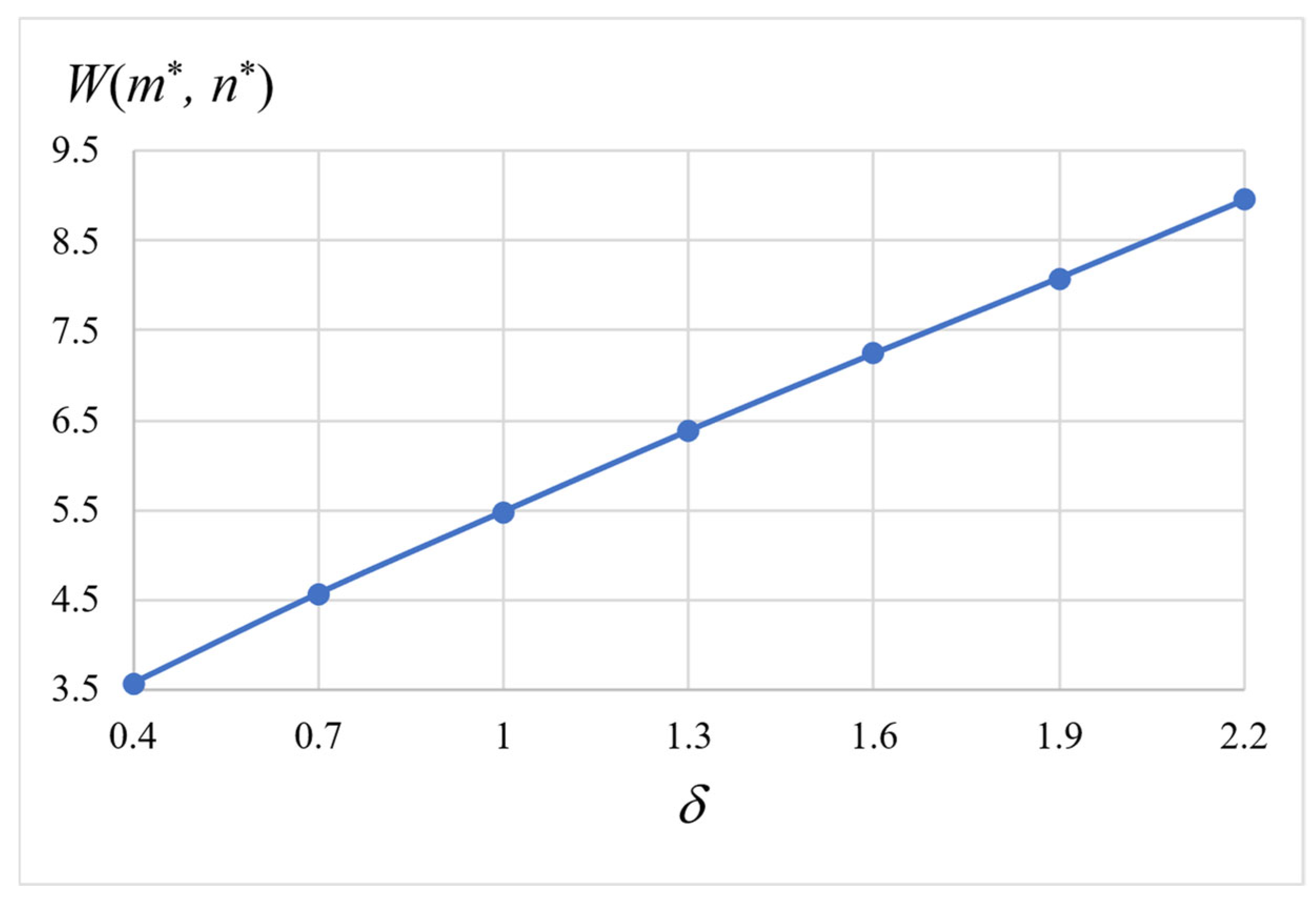
Figure 5 and Figure 6 illustrate the effect of the MS deterioration rate $\delta$ on the entire system. Figure 5 shows that, as can be expected, $W(m^{*},n^{*})$ increases linearly with the MS’s deterioration rate. Figure 6 shows that $n^{*}$ decreases at a diminishing rate with the increase in $\delta$, and $m^{*}$ only slightly decreases with the increase in $\delta$. The question that arises is how an increase in $\delta$ affects the $Ef{f}_{n+1}$ (the MS’s efficiency upon leaving for a vacation). Obviously, on the one hand, an increase in $\delta$ has a negative effect on $Ef{f}_{n+1}$, but on the other hand, $n^{*}$ decreases with $\delta$, which has positive effect on $Ef{f}_{n+1}$. Figure 6 also shows that $Ef{f}_{n+1}$ decreases with the increase in $\delta$. This means that the main server compensates for the increasing loss of efficiency by reducing the number of services in each cycle; however, this loss is not totally compensated for.

Figure 7 and Figure 8 illustrate the effects of changes in the recovery rate b on the system’s parameters. Figure 7 shows that, as can be expected, $W(m^{*},n^{*})$ decreases linearly with the increase in the MS’s recovery rate. Figure 8 shows that both $m^{*}$ and $n^{*}$ are almost entirely robust to changes in b. This result can be explained by the vacation time, which acts as a function of b (see Equation (18)).

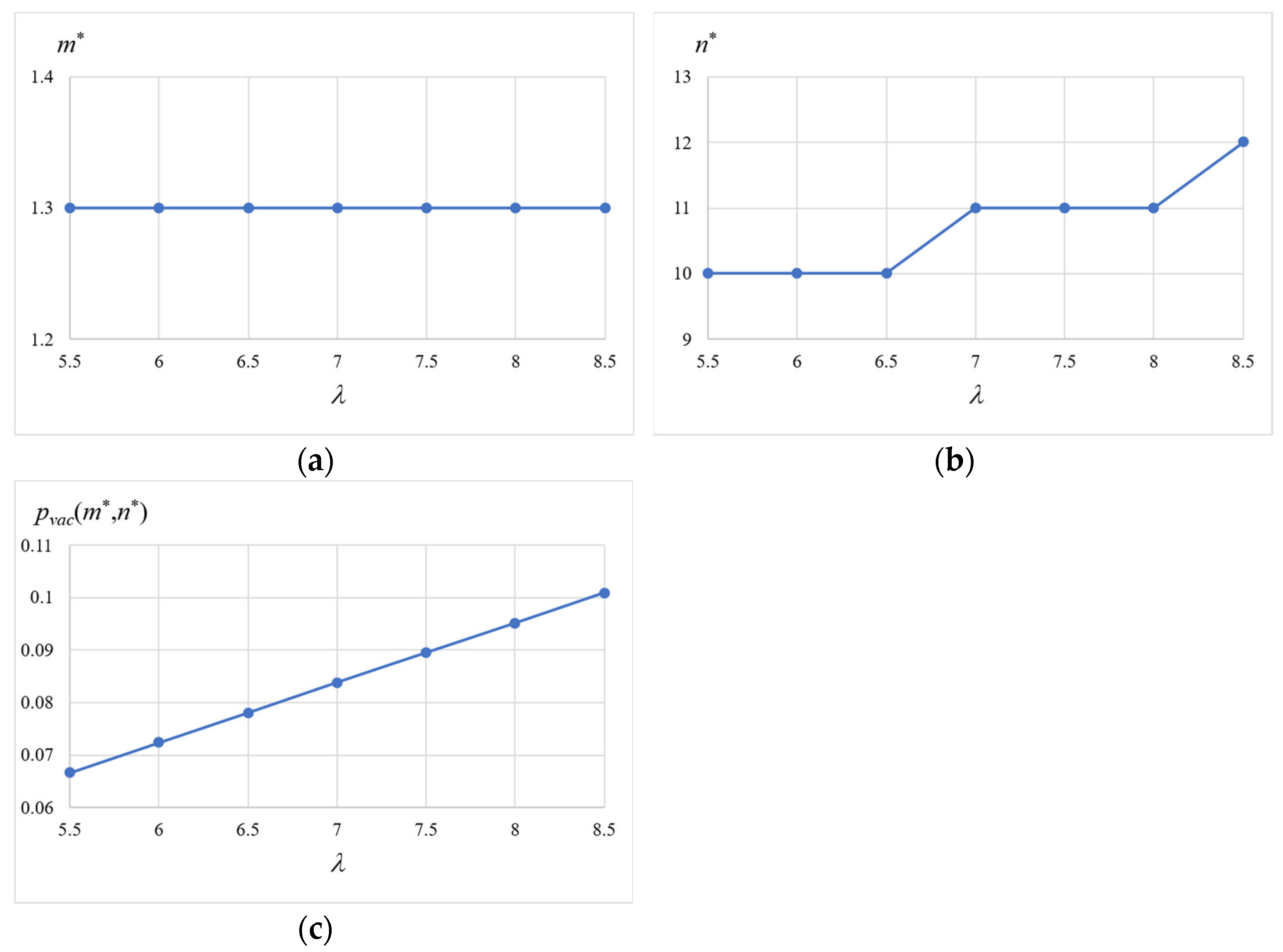
Finally, Figure 9 and Figure 10 present the effects of various customers’ arrival rates $\lambda$ on the system. As can be expected, Figure 9 shows that $W(m^{*},n^{*})$ increases linearly with the increase in the customers’ arrival rate, while Figure 10 shows that $m^{*}$ is totally robust to changes in $\lambda$, and $n^{*}$ slightly increases with the increase in $\lambda$. Interestingly, the figure shows that $p_{vac}(m^{*},n^{*})$ slightly increases with $\lambda$. This result can be explained as follows: as more customers arrive and enter the system, the MS is less idle during the time in which he/she/it is in the system and thus spends less time in the system.

4. Model with a Surviving Server

In this section, we consider a service system where the server is able to operate with no vacations at all; thus, he/she/it can decide whether or not to leave for a vacation. In what follows, we compare these two options. In particular, we use the classical M/M/1 queue as a baseline for comparison. Let ${\mu }_k=\mu (c(\delta )+Ef{f}_k)$ be the service rate of the $k^{th}$ customer, where $c(\delta )$ is the deteriorating function of $\delta$. Note that $c(\delta )$ is a constant, since $\delta$ is a given parameter of the system. It was shown in the previous section that $Ef{f}_k\underset{\hspace{1em}k\to \infty \hspace{1em}}{\to }0,$ and as a consequence, we obtain ${\mu }_k\underset{\hspace{1em}k\to \infty \hspace{1em}}{\to }\mu c(\delta )$. Thus, if $\mu c(\delta )>\lambda$, the system can operate after a sufficient time as a classic M/M/1 system without vacations. In the following pages, we investigate the level of improvement achieved using a policy that includes vacations. Let $W_{M/M/1}=1/(\mu c(\delta )-\lambda )$ be the customers’ sojourn time in a classical M/M/1 system with a service rate of $\mu c(\delta )$ and arrival rate of $\lambda$. Let $\xi$ be the percentage improvement of the proposed vacation model relative to the classical M/M/1 model, which is given by

$$\xi =\frac{W_{M/M/1}-W(m^{\ast },n^{\ast })}{W_{M/M/1}}\times 100.$$

Sensitivity Analysis

In order to investigate the effect of each parameter on $\xi$, we use the following parameter values as a base example: $\lambda =8$, $\mu =1$, $\beta =9$, $\delta =1$, $b=5$, $c=10/{\delta }^{0.1}$, $m_{\max }=1.8$. We calculate $\xi$ for various values of these parameters, where we change a single parameter in the system each time. The results are presented in Figure 11, Figure 12, Figure 13, Figure 14 and Figure 15. Figure 11 shows that $\xi$ linearly increases with $\beta$, meaning that using the vacation as a tool for improving the system’s efficiency is more beneficial, as the TS’s service rate is higher. Figure 12 shows that $\xi$ convexly increases with $\delta$. This result indicates that the increase in $\delta$ has a more significant negative effect on the M/M/1-type system compared with the proposed vacation system. Figure 13 shows (as expected) that $\xi$ increases linearly with the increase in the recovery constant b. Finally, Figure 14 shows that $\xi$ convexly increases with $\lambda$, indicating that the vacation model becomes beneficial in busy systems, where $\lambda$ approaches its upper limit. Finally, Figure 15 illustrates how the gap between the sojourn times of the two types of systems grows ($W(m^{*},n^{*})$ for the vacation model and $W_{M/M/1}$ for the M/M/1 model).

Figure 11. $\xi$ for various values of β.

Figure 12. $\xi$ for various values of δ.

Figure 13. $\xi$ for various values of b.

Figure 14. $\xi$ for various values of λ.

Figure 15. $W_{M/M/1}$ and $W(m^{*},n^{*})$ for various values of $\delta$.

5. Conclusions

In this study, we investigated a deterioration in a server’s efficiency, which commonly occurs in service systems operated by a human or machine server. To compensate for this loss of efficiency, the server leaves for a vacation, during which his/her/its efficiency is recovered. During the vacation, a temporary server with inferior efficiency provides services. Using probabilistic methods, we calculated the steady state probabilities and obtained the performance measures. Applying economic analysis, the study found that the customer sojourn time with the proposed model was improved by up to 80% over the non-stop working model. This study can be extended by considering the deterioration of the temporary servers’ efficiency as well as using multiple servers. A further study could consider the utilization of the server’s idle time when the system is empty of customers and the server is not on vacation. Although the benefits of the proposed method have been clearly demonstrated, it can be further improved by considering more accurate human factors such as deterioration and recovery rates of efficiency due to service intensity, as well as considering the adjustment of the server to service after returning from a vacation.