Abstract
In this work, by considering spatial uniform meshes and stencils having five adjacent discretization nodes, we furnish a numerical scheme to solve the time-fractional Black–Scholes (partial differential equation) PDE to price financial options under the generalized multiquadric radial basis function (RBF). The time-fractional derivative is estimated by an L1-scheme but the spatial variable is discretized using fourth-order RBF-FD methodology. As a matter of fact, the PDE problem is transformed in the form of a linear set of algebraic equations. To support analytical discussions, numerical tests are furnished and reveal the efficacy of the presented solver.
Keywords:
option pricing; fractional Black–Scholes; radial basis function (RBF); RBF-FD; numerical method MSC:
65M22; 35R11
1. Preliminaries and Literature
The topic of computational methods in resolving partial differential equations (PDEs) of the fractional type is an active area of research with a wide range of applications in various fields. Let the real function a be continuous and v be a constant, then the modified Riemann–Liouville (RL) fractional differentiation has the following definition [1]:
where is the Gamma’s function. In addition, the Caputo fractional derivative can be expressed as [2]:
By considering the (right) modified Riemann–Liouville (RL) time derivative, the Black–Scholes (BS) option price in the fractional sense could be given as comes next (forward in time) [3,4]:
wherein is the maturity time, the rate of interest is r and . Moreover, are scalars. Here, y is unbounded from one side. Additionally, is the real Hurst exponent and , [5]. It is clear that (3) would yield in the classical BS PDE by considering .
The initial condition for (3) can be, respectively, given by the put and call vanilla options as comes next [6] (Chapter 1):
and
wherein K is the price of strike. Here, the symbol of + stands for the function .
Note that the stochastic integrals under the Itô theory cannot be used since the fractional Brownian motion (FBM) is a semi-martingale. In fact, as the underlying market is driven by FBM, it must be clarified how to ensure the unique price of the market, as for this market, in the absence of transaction costs (taxes, commissions, etc.), there could still be an arbitrage strategy. In this paper, we follow the approach presented in [7,8,9], where the authors introduce the concept of a centered Gaussian martingale, referred to as the fundamental martingale. They demonstrate that this martingale produces the same filtration as the FBM. Given that the filtration captures the market information rather than the stochastic process alone, it is sensible to utilize this martingale for option pricing purposes.
On the other hand, one of the fundamental computational schemes for resolving the fractional BS PDE is the finite difference (FD) scheme [10] (Part IV) [11,12], which is mostly via equidistant discretization points and transforming the (3) into a system of discrete ones. To discuss this further, a spectral method for solving time-fractional PDEs in mathematical finance has been introduced in [13]. Recently, the FD method has been proposed in the compact form for solving the temporal-fractional BS PDE in [14].
Another type of numerical method that has attracted the attention of researchers is the meshfree method, see, for example, [15] and the references therein. Radial basis function (RBF) methods are a category of meshfree schemes that have been divided into two main categories of local and global ones. The local RBF meshfree method has the advantage of the sparse matrices when doing the discretizations. Another well-resulted approach that inherits both from the RBF and FD methods is the localized RBF-FD scheme [16,17]. The appearance and progressively comprehensive adoption of meshfree RBF-FD methods submit supplementary opportunities to reduce the computational cost when dealing with arbitrary domains in high dimensions.
In some works from the literature, such as [18], a logarithmic transformation is first performed on the fractional BS PDE to transform it into a PDE with constant coefficients. Although this may be useful at first sight, its problematic issue is that it makes the transformed PDE be defined on unbounded domains from both sides. This makes the application of numerical methods and the incorporation of boundary conditions more challenging. Thus, we do not perform such an act here in this work.
The major aim of this study is to pursue the recent literature [19,20] and present an effective numerical method for resolving (3) with the help of a well-known and general RBF, i.e., the generalized multiquadric (GMQ) RBF. We are here motivated to propose a new method-based RBF-FD methodology, which is based on a general family of RBF and can contain different types of RBFs as well as has fourth order of convergence on stencils having five uniform discretization points.
The remaining portions of this work unfold as follows:
- Section 2 is assigned to three parts, in which the first part discusses the fractional temporal discretization, while the second and the third parts are for the RBF-FD methodology and obtaining the weighting coefficients for a stencil having five nodes.
- Section 2 also furnishes a quartically convergent discretization for the space variable (i.e., the underlying asset) by using five adjacent uniform points.
- Section 3 studies how the presented method could be derived in matrix notations for the convenience of the users.
- Section 4 is furnished to put on show the comparisons of our solver in contrast to the state-of-the-art solvers of the same type.
- Section 5 gives brief conclusions of this manuscript with several outlines for forthcoming works.
2. Discretizations
2.1. Temporal Discretization
Assuming that the mesh of time discretization nodes is given on with equidistant increments . The work [21] gives the L1 scheme in the calculation of the differentiation in the fractional RL sense on a as follows:
where the weights can be extracted from
Noting that for the uniform stencils, the L1 scheme might be furnished as follows:
2.2. RBF-FD Formulation
Let us assume L as a linear operator. For calculating in the RBF-FD at for the point locations , we write down [22]:
where indicates a vector quantity in d as its dimension for . Here, the weights are the RBF-FD weights obtained by considering a stencil and then imposing the RBF and its derivatives to find them. As discussed in [22], for the appropriate choice of the shape parameter and the RBF, the resulting linear system obtained through (9) is invertible and the weights can be obtained both theoretically and numerically. We here focus on finding and using the weights in their closed form since finding them numerically will cause both higher CPU time and instability. Here, although L is a linear operator, it can be proved that to obtain the weights in the RBF-FD methodology, this operator will finally only act on the right-hand side vector, and the matrix in (9) is constructed based on the stance matrix.
2.3. Spatial Discretization Nodes
Now, we take into account the famous GMQ RBF as comes next [23,24]:
for a suitable value, l, indicates the Euclidean distance and p is the parameter of shape. In this work, we examine a stencil comprising n scattered nodes. To determine the weights for the RBF-FD methodology, we formulate the following expression at a given point :
where is the number of knots inside the stencil. The purpose here is to obtain the weights of the GMQ RBF-FD scheme for a stencil with five discretization points. Hence, it is taken into account that:
is an equally-spaced stencil. To compute the weights associated with the estimation of the first derivative, one now considers
Here, are the weights in this case. Substituting the function a by (10), centered at , , , , and gives a set of symbolic linear equations as follows:
The system (14) can be written as: where
and
Thus, the weighting coefficients of the GMQ RBF-FD technique to estimate when can be simplified and presented as follows:
Here, the term “simplified” means that the weights constructed through the RBF-FD methodology (11) are a bit bulky and contain many terms. Hence, to make the weights more revealing and useful in practice, we employ a Taylor expansion on them around zero by having the condition . Now, the error equation can be obtained by putting back the weights into the approximation formula (13) and writing Taylor expansion up to the desired order:
where .
For finding the approximation of the second derivative using RBF-FD methodology, we write
Similarly, as described above, we attain the weighting coefficients as follows:
with
and
The error equation, in this case, can be obtained as follows:
where and
The approximated formulas are used for the practical fractional PDE problem (3) and it is discussed how they can help our numerical method to possess faster convergence in Section 4. To judge the quality and effectiveness of the proposed method and the potential advantages with respect to the existing methods, it is also remarked that due to employing five adjacent nodes in (11), we are able to construct linear systems consisting of five equations with five unknowns theoretically and then obtain the weights by solving the system analytically. The weights can one time be programmed and then each time the five adjacent points change the weights will be changed and fill the appropriate row of a differentiation matrix. This procedure saves computational time as well as reduces the instability that occurs in finding the weights numerically for each set of five adjacent points. Although we focused on finding the weights for the first and second derivatives, the weights for higher-order derivatives can also be computed, which are not provided here since we focus on solving a second-order PDE. Furthermore, currently, we are unable to provide an analysis of the error bounds theoretically.
3. The Proposed Solver in Matrix Notation
By denoting we can write a full discretization scheme for (3) in what follows:
It is now possible to write down
Noting that the application of the fourth-order RBF-FD formulations given in Section 2.3 will arise in sparse differentiation matrices having penta-diagonal structure.
To follow our procedure more carefully and make the contribution by furnishing an efficient method in matrix notations, let us put all the differentiation weights into appropriate matrices of proper dimensions. For the weights associated with the first and the second derivatives, we can write down
and
It is remarked that for the nodes in which the central RBF-D formulas given in Section 2.3 are not valid, one may derive similar RBF-FD weights using similar methodology given therein. Now, we are in a position to write down and fill up the following matrix:
wherein ⊗ stands for the product of Kronecker [25] and
Noticing that
is an unit matrix, while and are and unit matrices, respectively. Therefore, the time-fractional PDE (29) can be discretized fully through:
wherein
Let us consider:
Therefore, we obtain . Noting that now for put and call options, the boundary conditions could be written, respectively, as [20]:
wherein is a large positive scalar. Ultimately, the whole numerical discretization procedure for resolving the time-fractional BS PDE (29) could be simplified in the form of an algebraic linear system of equations as comes next:
where, respectively, and are the system matrix and its associated vector after imposing the initial and boundary conditions. Moreover, B contains the vector of unknowns after having the Kronecker product. After having a theoretical discussion in this section about how to construct the proposed method in matrix form as a linear system of equations, it is now time to move on and test it on different types of input values on (3). This is the concept of the next section.
The differentiation matrix corresponding to the L1 scheme is an M-matrix (i.e., it is a Z-matrix with eigenvalues whose real parts are non-negative), which makes invertible. On the other hand, A in (33) is non-singular since no zero rows two so much close knots are thereby in the spatial discretization (under appropriate choices of the financial parameters in (3)). Thus, the system matrix in (39) is invertible.
The whole computational high-order method can be summarized in Algorithm Section 3.
| Algorithm 1 Solving the temporal-fractional BS PDE |
|
4. Computational Results
This section is devoted to re-check the discussions given in Section 2 and Section 3 by pricing some financial options when . To this goal, several famous solvers are compared such as:
- The fundamental FD method on uniform meshes with quadratic convergence rate along space and the first order of discretization along time given in [18] and denoted by FDM2.
- The first published work based on the RBF-FD methodology on equally-spaced meshes for solving (3) in [20] and shown by RBF-FD2.
- Our proposed solver based on uniform meshes but with quartical convergence along space and the RBF-FD methodology and first-order discretization along the fractional temporal variable shown by RBF-FD4.
Our laptop specifications are Windows 11 with Intel Core i7-12700H RTX 3070. Mathematica 13.0 [26,27] is employed to do the implementations and solve the linear system of equations using automatic built-in commands. The elapsed CPU time is furnished in seconds. Additionally, the absolute error is given by:
wherein and are the referenced and computational solutions, respectively.
One of the effective ways for obtaining a proper shape parameter can be used as .
Example 1.
Using the following set of parameters, here we investigate the efficacy of different methods for call option pricing:
The price of reference is , [20].
Table 1 is provided to compare the behavior of various solvers in resolving the fractional problem (3). Three types of solvers have been compared. The standard second-order FD method along with the second-order RBF-FD method over non-uniform stencils and the proposed high-order RBF-FD scheme with fourth order of convergence. The presented scheme beats the other solvers in terms of accuracy and CPU time. To also check the stability and positivity of the presented method, it is necessary to observe the numerical solutions for different numbers of discretization nodes in the computational domain. This is performed in Figure 1. In Figure 1, we give the numerical solution based on two sets of discretization points. The knots are uniform. The list point plots are given on the left, which is the numerical solution in the discrete format while the right figures have been drawn by passing an (automatically generated via the software Mathematica 12.0) interpolated solution in the continuous mode.

Table 1.
Computational comparisons given for various solvers under Example 1.
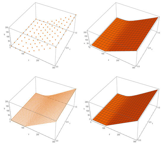
Figure 1.
Numerical reports in Example 1 for RBF-FD4. (Top Left): The point plot when . (Top Right): The continuous plot when . (Bottom Left): The point plot when . (Bottom Right): The continuous plot when .
Example 2.
Using the following set of parameters, here we investigate the efficacy of the different for the put option pricing:
The reference price is ,20].
Computational reports for this test are furnished in Table 2 reconfirming the efficacy of the proposed RBF-FD solver with fourth order of convergence along space. Furthermore, we showcase the numerical solution in Figure 2, demonstrating the robustness and stability of our proposed solver while also highlighting its inherent positivity. Again, in Figure 2, when uniform knots are considered, and Algorithm 1 is followed in order to obtain the numerical solution. The left figure shows the numerical solution in the discrete mode while the right one is the continuous interpolated numerical solution.
Table 2.
Computational comparisons given for various solvers under Example 2.
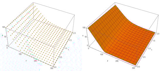
Figure 2.
In Example 2, we present numerical results for RBF-FD4. On the (left), we provide a point plot for the case of . On the (right), we display a continuous plot of the solution for the same set of .
The rationale behind using or is to consider the fractional value of the derivative in (3) and test the efficiency of the proposed method for such values, which makes the Hurst index two different values on the fractional Brownian motion in modeling the data.
5. Concluding Remarks
In this work, to solve temporal-fractional option pricing PDE problems arising in finance, we introduced the weights for the GMQ RBF-FD methodology on stencils having five uniform discretization points. The temporal-fractional PDE problem was transformed by fourth-order discretizations coming from the RBF-FD methodology along the spatial variable and the L1 scheme for the discretization along the time variable. The solver was proposed in matrix notations to simplify the whole procedure. To the best of our knowledge, this is the first paper that employed fourth-order local RBF-FD approximations on solving the temporal fractional BS PDE under the GMQ RBF. Numerical tests were considered and solved in Section 4. Computational results clearly showed that the proposed solver increase the accuracy of the final approximations. Some further remarks are in order:
- Forthcoming works might concentrate on deriving super-efficient solvers based on the Hermite idea to increase the speed of convergence without adding further stencil nodes in solving time-dependent PDEs.
- We too investigate extending the applicability of the L2 scheme in estimating the temporal fractional derivative to obtain higher-order accurate approximations for the time-fractional PDE (29).
Author Contributions
Conceptualization, M.Z.U., A.K.A. and H.M.A.; formal analysis, A.K.A. and H.M.A.; funding acquisition, M.Z.U. and S.S.; investigation, A.K.A. and S.S.; methodology, A.K.A. and H.M.A.; supervision, M.Z.U. and S.S.; validation, M.Z.U., A.K.A. and S.S.; writing—original draft, S.S. and H.M.A.; writing—review & editing, A.K.A. and H.M.A. All authors have read and agreed to the published version of the manuscript.
Funding
This research recieved no external funding.
Institutional Review Board Statement
Not applicable.
Informed Consent Statement
Not applicable.
Data Availability Statement
Not applicable.
Acknowledgments
This research work was funded by Institutional Fund Projects under grant no. (IFPIP: 1316-130-1443). The authors gratefully acknowledge technical and financial support provided by the Ministry of Education and King Abdulaziz University, DSR, Jeddah, Saudi Arabia.
Conflicts of Interest
The authors confirm that they have no personal relationships or competing financial interests that could have influenced the integrity and objectivity of the research presented in this manuscript.
References
- Jumarie, G. Modified Reimann-Liouville derivative and fractional Taylor series of non-differentiable functions further results. Comput. Math. Appl. 2006, 51, 1367–1376. [Google Scholar] [CrossRef]
- Caputo, M. Linear model of dissipation whose Q is almost frequency independent II. Geophys. J. Int. 1967, 13, 529–539. [Google Scholar] [CrossRef]
- Wyss, W. The fractional Black-Scholes equation. Fract. Calc. Appl. Anal. 2000, 3, 51–62. [Google Scholar]
- Jumarie, G. Derivation and solutions of some fractional Black-Scholes equations in coarse-grained space and time: Application to Merton’s optimal portfolio. Comput. Math. Appl. 2010, 59, 1142–1164. [Google Scholar] [CrossRef]
- Hurst, H.E. Long-term storage capacity of reservoirs. Trans. Amer. Soc. Civil Eng. 1951, 116, 770–799. [Google Scholar] [CrossRef]
- Seydel, R.U. Tools for Computational Finance, 6th ed.; Springer: London, UK, 2017. [Google Scholar]
- Norros, I.; Valkeila, E.; Virtamo, J. A Girsanov-type formula for the fractional Brownian motion. In Proceedings of the First Nordic-Russian Symposium on Stochastics, Helsinki, Finland, 14–16 August 1996. [Google Scholar]
- Norros, I. Four approaches to the fractional Brownian storage. In Fractals in Engineering; Lévy Véhel, J., Lutton, E., Tricot, C., Eds.; Springer: London, UK, 1997; pp. 154–169. [Google Scholar]
- Feyel, D.; de la Pradelle, A. On fractional Brownian processes. Potential Anal. 1999, 10, 273–288. [Google Scholar] [CrossRef]
- Duffy, D.J. Finite Difference Methods in Financial Engineering: A Partial Differential Equation Approach; Wiley: Hoboken, NJ, USA, 2006. [Google Scholar]
- Heston, S.L. A closed-form solution for options with stochastic volatility with applications to bond and currency options. Rev. Finan. Stud. 1993, 6, 327–343. [Google Scholar] [CrossRef]
- Itkin, A. Pricing Derivatives Under Lévy Models: Modern Finite-Difference and Pseudo-Differential Operators Approach; Birkhäuser: Basel, Switzerland, 2017. [Google Scholar]
- An, X.; Liu, F.; Zheng, M.; Anh, V.V.; Turner, I.W. A space-time spectral method for time-fractional Black-Scholes equation. Appl. Numer. Math. 2021, 165, 152–166. [Google Scholar] [CrossRef]
- Roul, P.; Prasad Goura, V.M.K. A compact finite difference scheme for fractional Black-Scholes option pricing model. Appl. Numer. Math. 2021, 166, 40–60. [Google Scholar] [CrossRef]
- Hon, Y.C. A quasi-radial basis functions method for American options pricing. Comput. Math. Appl. 2002, 43, 513–524. [Google Scholar] [CrossRef]
- Bollig, E.F.; Flyer, N.; Erlebacher, G. Solution to PDEs using radial basis function finite-differences (RBF-FD) on multiple GPUs. J. Comput. Phys. 2012, 231, 7133–7151. [Google Scholar] [CrossRef]
- Liu, T.; Ullah, M.Z.; Shateyi, S.; Liu, C.; Yang, Y. An efficient localized RBF-FD method to simulate the Heston-Hull-White PDE in finance. Mathematics 2023, 11, 833. [Google Scholar] [CrossRef]
- Zhang, H.; Liu, F.; Turner, I.; Yang, Q. Numerical solution of the time fractional Black-Scholes model governing European options. Comput. Math. Appl. 2016, 71, 1772–1783. [Google Scholar] [CrossRef]
- Yang, P.; Xu, Z. Numerical valuation of European and American options under fractional Black-Scholes model. Fractal Fract. 2022, 6, 143. [Google Scholar] [CrossRef]
- Song, Y.; Shateyi, S. Inverse multiquadric function to price financial options under the fractional Black-Scholes model. Fractal Fract. 2022, 6, 599. [Google Scholar] [CrossRef]
- Diethelm, K. An algorithm for the numerical solution of differential equations of fractional order. Electron. Trans. Numer. Anal. 1997, 5, 1–6. [Google Scholar]
- Bayona, V.; Moscoso, M.; Carretero, M.; Kindelan, M. RBF-FD formulas and convergence properties. J. Comput. Phys. 2010, 229, 8281–8295. [Google Scholar] [CrossRef]
- Sarra, S.A.; Chenoweth, M.E. A numerical study of generalized multiquadric radial basis function interpolation. SIAM Undergrad. Res. Online 2009, 22, 58–70. [Google Scholar]
- Soleymani, F.; Ullah, M.Z. A multiquadric RBF-FD scheme for simulating the financial HHW equation utilizing exponential integrator. Calcolo 2018, 55, 51. [Google Scholar] [CrossRef]
- Zhang, H.; Ding, F. On the Kronecker products and their applications. J. Appl. Math. 2013, 2013, 296185. [Google Scholar] [CrossRef]
- Soleymani, F.; Akgül, A. European option valuation under the Bates PIDE in finance: A numerical implementation of the Gaussian scheme. Disc. Cont. Dyn. Sys. Ser. S 2020, 13, 889–909. [Google Scholar] [CrossRef]
- Wellin, P.R.; Gaylord, R.J.; Kamin, S.N. An Introduction to Programming with Mathematica; Cambridge University Press: Cambridge, UK, 2005. [Google Scholar]
Disclaimer/Publisher’s Note: The statements, opinions and data contained in all publications are solely those of the individual author(s) and contributor(s) and not of MDPI and/or the editor(s). MDPI and/or the editor(s) disclaim responsibility for any injury to people or property resulting from any ideas, methods, instructions or products referred to in the content. |
© 2023 by the authors. Licensee MDPI, Basel, Switzerland. This article is an open access article distributed under the terms and conditions of the Creative Commons Attribution (CC BY) license (https://creativecommons.org/licenses/by/4.0/).