A Complete Procedure for a Constraint-Type Fictitious Time Integration Method to Solve Nonlinear Multi-Dimensional Elliptic Partial Differential Equations

Abstract

In this paper, an efficient and straightforward numerical procedure is constructed to solve multi-dimensional linear and nonlinear elliptic partial differential equations (PDEs). Although the numerical procedure for the constraint-type fictitious time integration method overcomes the numerical stability problem, the parameter’s definition, numerical accuracy and computational efficiency have not been resolved, and the lack of initial guess values results in reduced computational efficiency. Therefore, the normalized two-point boundary value solution of the Lie-group shooting method is proposed and considered in the numerical procedure to avoid the problem of the initial guess value. Then, a space-time variable, including the minimal fictitious time step and convergence rate factor, is introduced to study the relationship between the initial guess value and convergence rate factor. Some benchmark numerical examples are tested. As the results show, this numerical procedure using the normalized boundary value solution can significantly converge within one step, and the numerical accuracy is better than that demonstrated in the previous literature.

1. Introduction

In actual engineering and science fields, partial differential equations (PDEs) are widely used to describe physical transfer behaviour. PDEs can be roughly divided into parabolic, hyperbolic and elliptic equations. According to the description of the characteristic curve, the characteristic line conveys the initial relevant information in parabolic and hyperbolic equations; on the contrary, since elliptic equations have no real characteristic line, no meaningful sense of information propagates for elliptic equations and no real characteristic line is widely described in the previous literature. In fact, the insubstantial characteristic line represents information that has lost its initial value. Nowadays, the most popular numerical methods, such as the finite difference method, finite element method, boundary element method and meshless (or mesh-free) method, are applied to solve the PDEs. Why can the numerical solution of these methods not be approximated to the true solution of the nonlinear PDEs found so far? The reason can be roughly divided into the discrete numerical technique and initial guess value problems. Up to now, most studies have focused on improving numerical methods for elliptic nonlinear problems, and there is no literature exploring the initial guess value.

As mentioned above, to deal with elliptic boundary value problems (BVPs), most scholars have proposed different approximation functions and iteration methods to increase numerical accuracy and stability; for example, Atluri and Zhu [1] and Zhu et al. [2] proposed the meshless local Petrov–Galerkin method and the meshless local boundary integral equation method to solve nonlinear problems. Cheng et al. [3] proposed the exponential convergence method using the multiquadric and Gaussian radial basis functions for solving PDEs. Additionally, Cho et al. [4] applied a Trefftz method for solving parabolic, hyperbolic and parabolic–hyperbolic types of PDEs. Jin [5] used the method of fundamental solutions (called the F-Trefftz method) to solve the elliptic-type PDEs. Hu et al. [6] and Hu and Chen [7] used the radial basis collocation method and quasi-Newton iteration to address linear and nonlinear elliptic problems. Fan et al. [8] applied the modified Trefftz method to address two-dimensional Stokes problems. Zhang et al. [9] proposed a new mesh-free method for solving Burgers’ equation with various viscosity values. The numerical solutions obtained with different viscosity values have been compared with the analytical solutions and the results of other numerical schemes. The comparative results indicate that the proposed method is an efficient, robust and reliable way of solving Burgers’ equation. Seydaoğlu [10] proposed solving the one-dimensional Burgers’ equation based on the multiquadric radial basis function for space approximation and the Lie-group scheme for time integration. The result shows that the proposed algorithm is efficient and can be easily implemented. To increase the rate of convergence, a stochastic approach [11] based on the Monte Carlo method with a random walk technique and the Fokas method [12] (called the unified transform method) was developed to solve elliptic problems. Recently, Ezeh and Kamoh [13] proposed a numerical approach based on the alternating-direction implicit (ADI) method to solve the two-dimensional Laplace equation. These numerical methods have significant calculation accuracy and efficiency for linear problems, but they inevitably have a large number of iterations and low calculation efficiency when encountering nonlinear BVPs. Furthermore, when the nonlinear problem surfs the noisy disturbance, these iteration methods will occur the numerical instability problem quickly.

To avoid iterative procedures under the noisy effect, Liu and Atluri [14] proposed a variable transformation, named the fictitious time integration method (FTIM), an extensive system of nonlinear algebraic equations. Liu [15] applied the FTIM to solve two-dimensional quasilinear elliptic boundary value problems. Furthermore, Ku et al. [16] modified the FTIM and considered a time-like function in the FTIM to increase the convergence rate. Later, Tsai et al. [17] applied the F-Trefftz method to solve Poisson-type nonlinear PDEs, and the FTIM with a time-like function was used to solve the linear algebraic equations. However, the selection of the parameters is difficult, such as the viscosity-damping coefficient, the fictitious time step and the convergence criterion. Furthermore, Chang [18] applied an FTIM for multi-dimensional backward heat conduction problems. Although these approaches seem to give a satisfactory result, there is a fatal problem with this method, which is the problem of multiple solutions. When the viscous damping coefficient, fictitious time step, convergence criteria and fictitious terminal time are not correctly selected, the FTIM will not converge and cause diverge. To avoid the numerical sensitivity problem of the initial guess value and parameter selection, some space-time variable transformations of methods, including the scalar-based homotopy method [19], manifold-based exponentially convergent algorithm [20], the residual-norm-based algorithm [21] and the dynamic Jacobian-inverse free method [22], have been proposed to avoid the actual sensitivity problem of the initial guess value. These approaches provide acceptable approximate results, but low convergence efficiency, and a large number of iterations are inevitable when considering strict convergence conditions or a large number of discrete grids.

Recently, Chen [23,24] applied an FTIM to solve multi-dimensional backwards-in-time heat conduction problems and successfully overcame the fictitious time step and convergence criterion problems over a long time span. However, for the parabolic type PDEs by the FTIM, an initial guess value depends on the final condition and determining the space-time coefficient problem still unresolved. Multiple solutions for solving elliptic PDEs will occur due to the lack of initial or termination conditions. As Chen [25] derived the forward and backward vector solution of the Lie-group shooting method (LGSM), the two-point solution of the LGSM is applied to the determination of the heat source and the initial data. The result shows that the iterative procedure depends on the initial guess value. Chen et al. [26] proposed a constraint-type FTIM to solve nonlinear multi-dimensional elliptic PDEs. To overcome the selection problems of the parameters, all parameters, including the viscosity-damping coefficient, system energy (the discrete number of grids) and minimum fictitious time size, were combined into a space-time constraint coefficient and introduced into the numerical procedure of the FTIM. The minimum fictitious time step can satisfy the continuity property and obtain a fast gradient along the integration path to approach the true solution. Although the constraint FTIM can satisfy the nonlinear algebraic equations and, at the same time, avoid the selection of the parameters, the relationship between the system energy, the initial condition (IC) definition and the convergence path is yet to be understood. According to reference [26], the initial guess values are constant without a definition, and the computational efficiency depends on the system energy of the space-time constraint coefficient. When the system energy and the discrete number of grids increase, the constraint FTIM struggles to obtain high numerical accuracy and computational efficiency. According to the two-point solution of the nonlinear dynamic system from the Lie-group shooting method, Chang et al. [27] applied it to determine the initial data of Burgers’ equation with a large Reynolds number. The result shows that the initial condition can be obtained within one step. Hence, this paper will propose a normalized boundary solution of the initial guess values from boundary conditions and define the system energy, independent of the discrete number of grids.

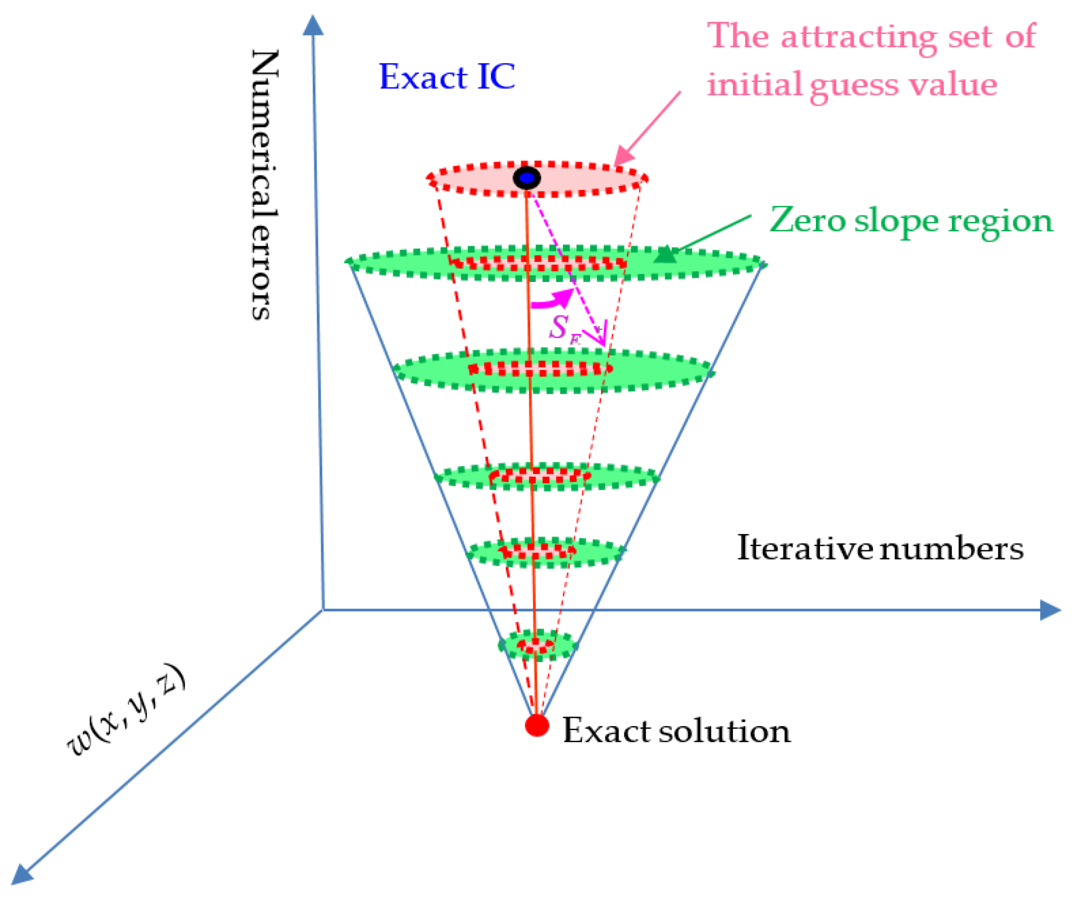
In this paper, we extend the work of Chen et al. [26]. A sketch of the convergence path of the constraint FTIM designed in this paper is shown in Figure 1. The two-point solution is applied to find the initial guess value from the boundary conditions, and the relationship between the convergence rate factor and the initial guess value is established. The remainder of this paper is organized as follows. Section 2 illustrates the mathematical formulation of the FTIM. In Section 3, we present several numerical examples, including linear and nonlinear Laplace equations, the nonlinear Poisson equation and nonlinear Helmholtz equation, to validate the proposed method. Finally, the conclusions are drawn in Section 4.

Figure 1. A sketch of the convergence path of the constraint FTIM.

2. Nonlinear and Nonhomogeneous Elliptic Equation

Let us consider the following equations:

$${\nabla }^{2}w\left(x,y,z\right)=F\left(x,y,z,w,w_x,w_y,w_z,\dots \right), \left(x,y,z\right)\in \mathsf{\Omega },$$

(1)

$$w\left(x,y,z\right)=B\left(x,y,z\right) \mathrm{on} \mathsf{\Gamma },$$

(2)

where $\nabla$ denotes a Laplacian operator, $\mathsf{\Gamma }$ is the boundary of the problem domain $\mathsf{\Omega }$, $w$ is a scalar field, and $F$ and $B$ are given functions.

2.1. Transformation into a New Evolutional PDE

First, consider the following variable transformation:

$$W\left(x,y,z,\tau \right)=\left(1+\lambda \right)w\left(x,y,z\right),$$

(3)

where $\lambda$ is a fictitious time variable.

According to Chen et al. [26], a space-time variable, $\xi$, is embedded into Equation (1):

$$0=-\xi {\nabla }^{2}w+\xi F\left(x,y,z,w,w_x,w_y,w_z,\dots \right),$$

(4)

where a constraint condition of the space-time variable is conducted as follows:

$$\frac{1}{\Delta \lambda }>\xi ,$$

(5)

$$\xi =\left(\frac{1}{\Delta \lambda ·E_{xyz}}\right), 0<\Delta \lambda <1, E_{xyz}>0,$$

(6)

where $E_{xyz}$ is a convergence rate factor based on the maximum discrete grid numbers in the space domain, and $S_E=1/E_{xyz}$ is defined as a convergence angle based on the convergence rate factor, as shown in Figure 1. If the initial condition knows, the result converges within one step, and $S_E$ approaches zero when the number of discrete grids increases. Here, the convergence rate and convergence angle can be used to observe whether the FTIM preserves the convergence path. When the number of discrete grids and $E_{xyz}$ increase, the numerical accuracy increases and the convergence speed decreases. On the contrary, the numerical accuracy decreases and the convergence speed increases.

Because $\partial W/\partial \lambda =w\left(x,y,z\right)$, Equation (4) can be added on both sides of the above equation as follows:

$$\frac{\partial W}{\partial \lambda }=\xi {\nabla }^{2}W-\xi \left(1+\lambda \right)F\left(x,y,z,w,w_x,w_y,w_z,\dots \right)+w.$$

(7)

Finally, by using $w=W/\left(1+\lambda \right),$ $w_x=W_x/\left(1+\lambda \right),$ $w_y=W_y/\left(1+\lambda \right)$ and $w_z=W_z/\left(1+\lambda \right),$ Equations (1) and (2) can be transformed into a new evolution parabolic-type PDE:

$$\frac{\partial W}{\partial \lambda }=\xi {\nabla }^{2}W-\xi \left(1+\lambda \right)F\left(x,y,z,\frac{W}{1+\lambda }, \frac{W_x}{1+\lambda },\frac{W_y}{1+\lambda },\frac{W_z}{1+\lambda },\dots \right)+\frac{W}{1+\lambda }, \left(x,y,z\right)\in \mathsf{\Omega },$$

(8)

$$W\left(x,y,z,\lambda \right)=\left(1+\lambda \right)B\left(x,y,z\right), \left(x,y,z\right)\in \mathsf{\Gamma }.$$

(9)

Applying a semi-discrete procedure to Equation (8) yields a coupled system of ODEs:

$$\begin{gathered} {\dot{W}}_{i,j,k}=\frac{\xi }{{\left(\Delta x\right)}^2}\left[W_{i+1,j,k}-2W_{i,j,k}+W_{i-1,j,k}\right] \\ +\frac{\xi }{{\left(\Delta y\right)}^2}\left[W_{i,j+1,k}-2W_{i,j,k}+W_{i,j-1,k}\right] \\ +\frac{\xi }{{\left(\Delta z\right)}^2}\left[W_{i,j,k+1}-2W_{i,j,k}+W_{i,j,k-1}\right] \\ -\xi \left(1+\lambda \right)F\left(x_i,y_j,z_k,\frac{W_{i,j,k}}{1+\lambda }, \frac{W_x}{1+\lambda },\frac{W_y}{1+\lambda },\frac{W_z}{1+\lambda },\dots \right)+\frac{W_{i,j,k}}{1+\lambda }, \end{gathered}$$

(10)

where $\Delta x,$ $\Delta y$ and $\Delta z$ are the uniform spatial lengths in the $x$, $y$ and $z$ directions, $W_{i,j,k}\left(\lambda \right)=W\left(x_i,y_j,z_k,\lambda \right),$ and $\dot{W}$ denotes the differential of $W$ with respect to $\lambda$.

2.2. The Convergence Criterion

The Euler method (EM) is applied to integrate Equation (10) starting from $\lambda =0$. In the numerical integration process, we can examine the convergence of $W_{i,j,k}$ at the $n$ and $n+1$ steps by

$$\sqrt{{\displaystyle \sum }_{i,j,k}^m{\left[W_{i,j,k}^{n+1}-W_{i,j,k}^n\right]}^2 \le \epsilon },$$

(11)

where $\epsilon$ is the selected criterion, m is the number of grid points in each spatial direction, and n is the iterative number in the fictitious time direction.

2.3. Normalized Initial Guess Value

According to Chen [25], who derived the forward and backward two-point vector solution from the LGSM, the initial data can be determined within one step. However, an initial value for the elliptic boundary value problem is missed; the normalized initial guess value on BCs can be represented as follows:

$${\mathrm{Z}}_{\mathsf{\Gamma }}=\frac{w}{\max \Vert w\Vert } \mathrm{on} \mathsf{\Gamma },$$

(12)

$$w^{*}=\max \Vert w_{\mathsf{\Gamma }}\Vert ·{\mathrm{Z}}_{\mathsf{\Omega }} \mathrm{on} \mathsf{\Omega },$$

(13)

where ${\mathrm{Z}}_{\mathsf{\Gamma }}$ denotes the initial value on BCs, $w^{*}$ is an initial guess value, and ${\mathrm{Z}}_{\mathsf{\Omega }}$ indicates the normalized initial value in the interior domain, which depends on BCs $\left({\mathrm{Z}}_{\mathsf{\Gamma }}\right)$.

3. Numerical Examples

3.1. Example 1

We first consider the following:

$${\nabla }^{2}w=0,$$

(14)

where $w\left(x,y\right)=e^x\cos y$ is an analytical solution of the Laplace equation, and BCs can be computed exactly.

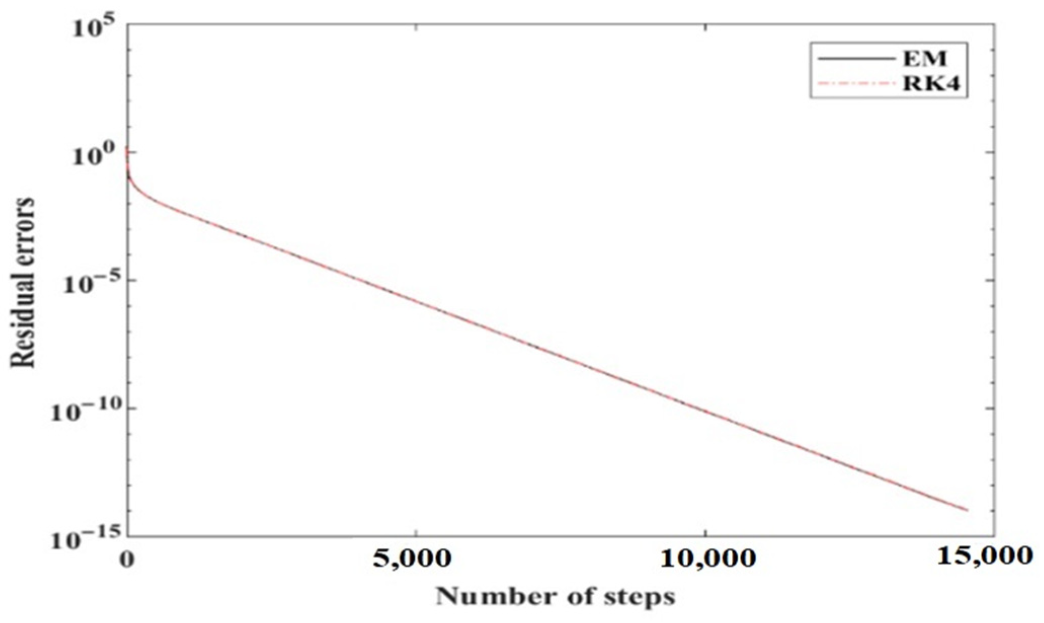
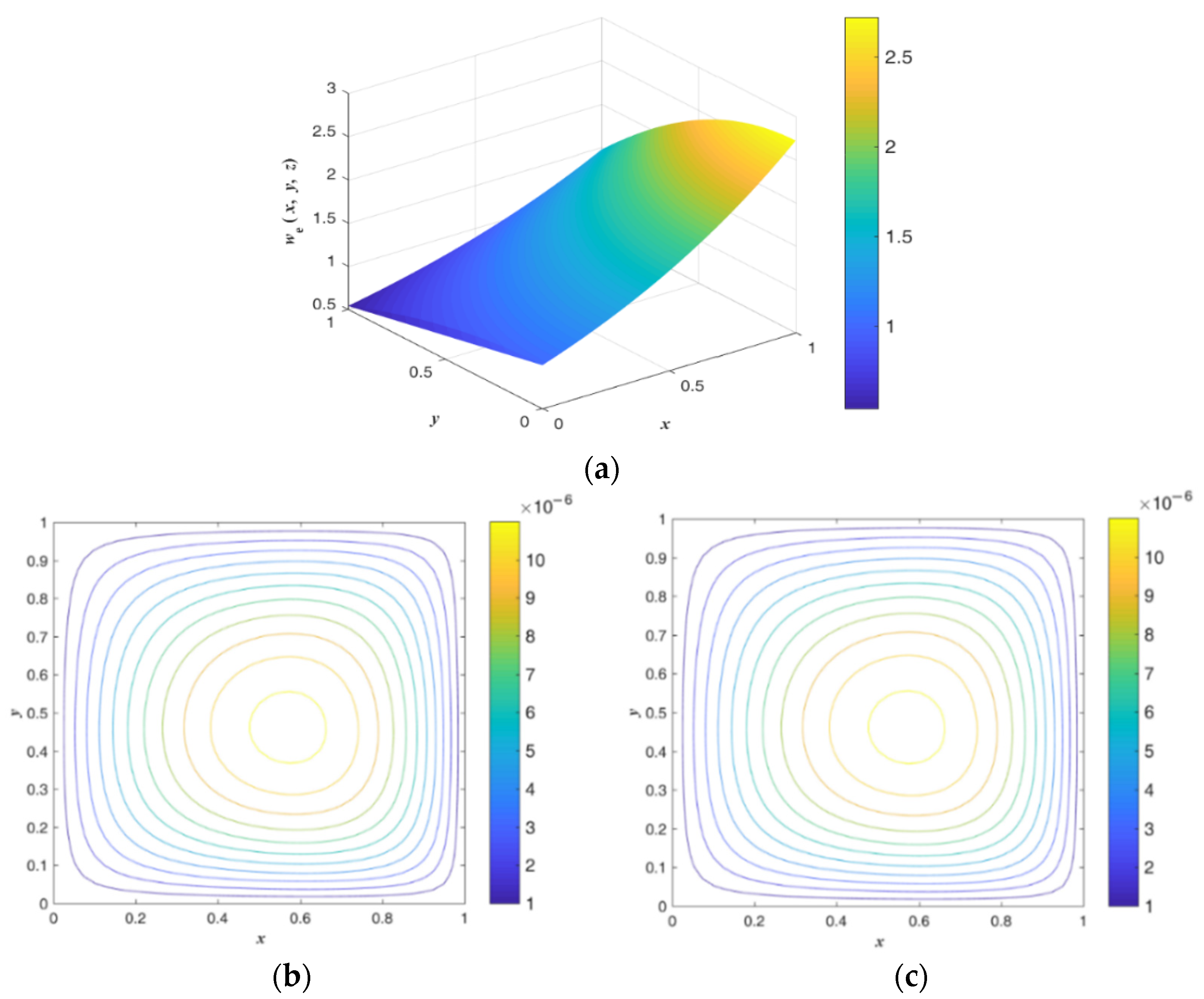
The domain is given by $\mathsf{\Omega }=\left\{\left(x,y\right)|0 \le x \le 1,0 \le y \le 1\right\}$. Here, we set the parameters as $N_x=N_y=41,$ $\Delta \mathsf{\lambda } ={10}^{-300},$ $\epsilon ={10}^{-14},$ $E_{xyz}={10}^4,$ and start from an initial guess value of $w_{i,j}=1$. In comparison with the Euler method (EM) and RK4, the convergence plot is shown in Figure 2. The proposed scheme converges for RK4 within $1.4567\times {10}^4$ and the EM within $1.4554\times {10}^4$ iterations. The absolute errors for RK4 and the EM are plotted in Figure 3, and both schemes have the same maximum errors of $1.136\times {10}^{-5}$. The absolute errors for RK4 and the EM are smaller than the values of $1.136\times {10}^{-5}$ in the proposed scheme and $4.9\times {10}^{-5}$ in the conventional FTIM by Liu [15]. As shown in Figure 1, the true solution depends on the initial guess value and $E_{xyz}$. That is, using higher-order numerical integration methods cannot improve numerical accuracy.

Figure 2. The convergence plot: red and black lines denote the RK4 and EM, respectively.

Figure 3. Potential distributions for a linear problem: (a) exact solution; (b) absolute errors of EM; (c) absolute errors of RK4.

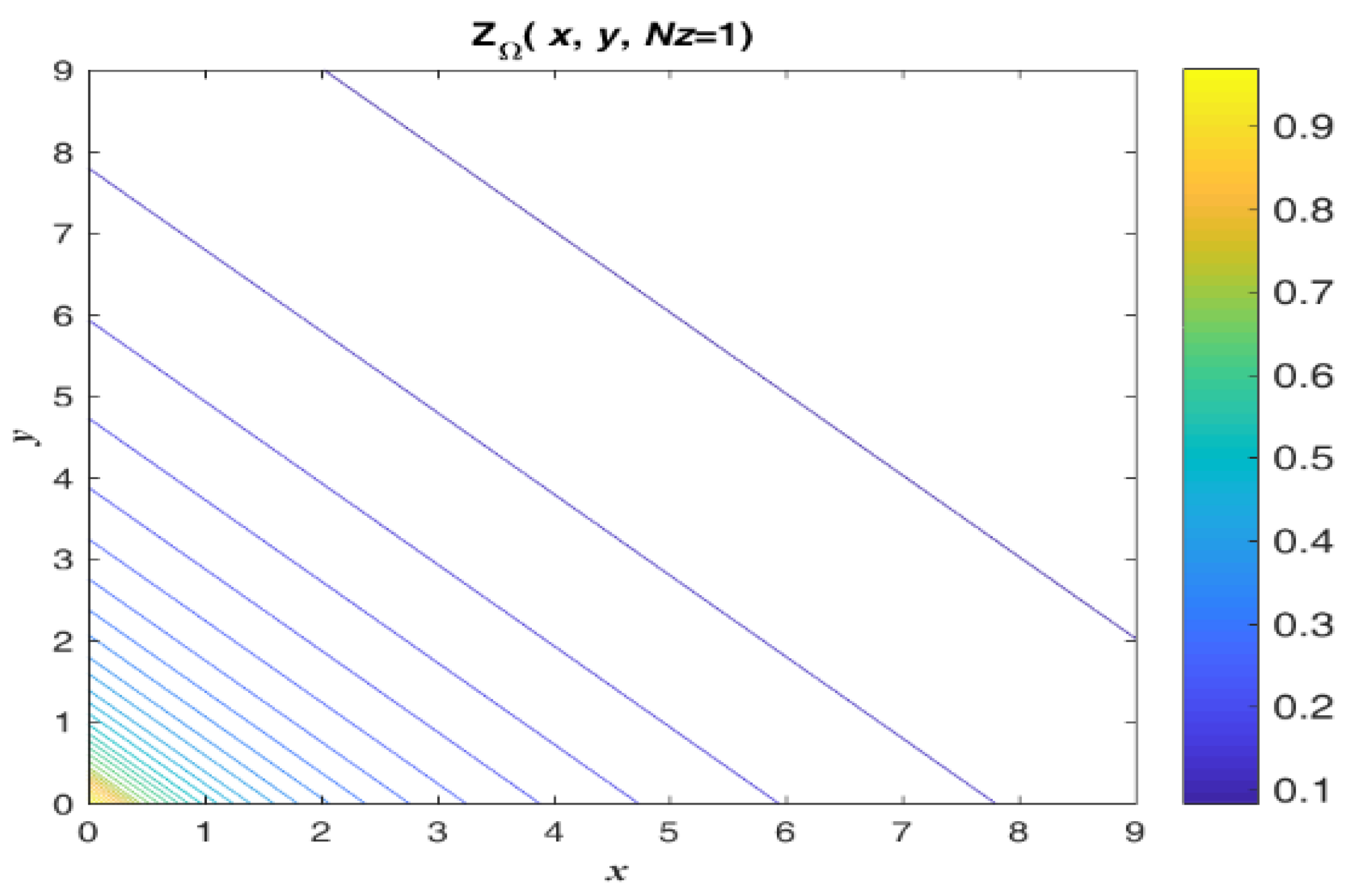
When testing different $E_{xyz}={10}^4$ and $E_{xyz}={10}^{14}$, the FTIM, starting from an initial value of $w^{*}= \max \Vert w_{\mathsf{\Gamma }}\Vert ·{\mathrm{Z}}_{\mathsf{\Omega }}$, is considered, as shown in Figure 4. The following linear formula can be used to address this issue:

$${\mathrm{Z}}_{{\mathsf{\Omega }}_4}={\mathrm{Z}}_{{\mathsf{\Gamma }}_3}\times \frac{{\mathrm{Z}}_{{\mathsf{\Gamma }}_2}}{{\mathrm{Z}}_{{\mathsf{\Gamma }}_1}},$$

(15)

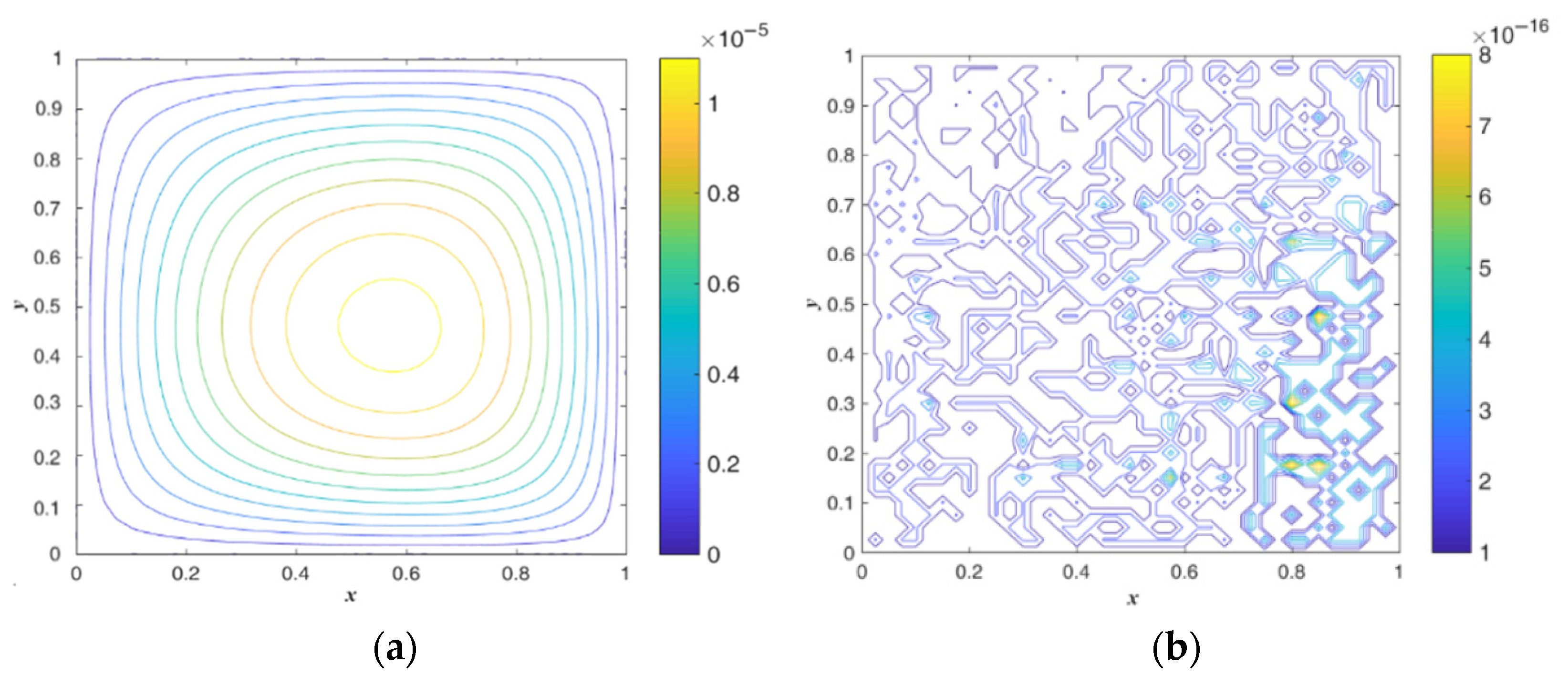
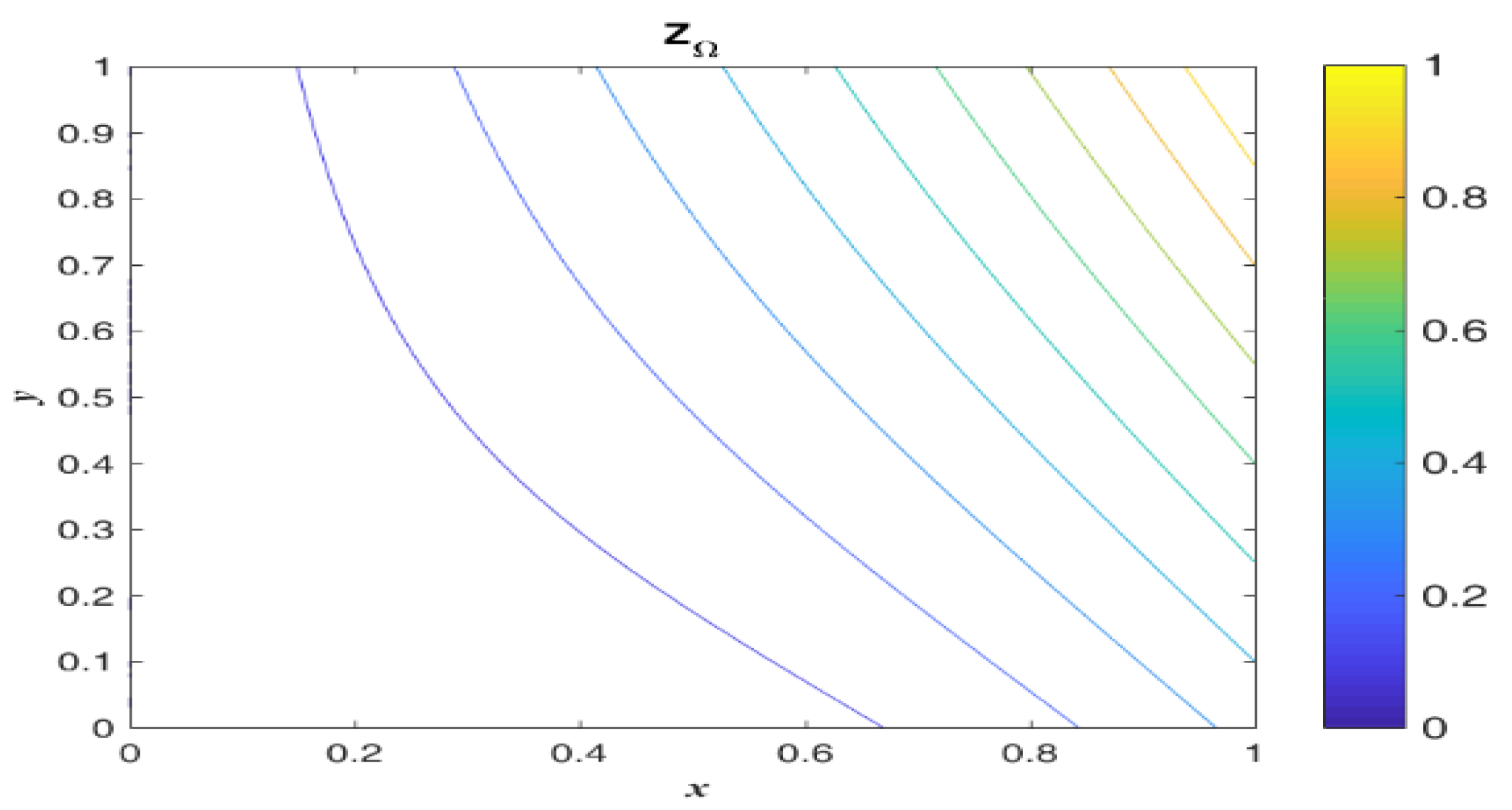
and the contour of the initial guess value of ${\mathrm{Z}}_{\mathsf{\Omega }}$ is shown in Figure 5. The convergence rate of the EM converges for $E_{xyz}={10}^4$ within $8.993\times {10}^3$ and $E_{xyz}={10}^{14}$ within one iteration. The absolute errors are shown in Figure 6, and the maximum error of the numerical solution is smaller than $1.1363\times {10}^{-5}$ for $E_{xyz}={10}^4$ and $8.8818\times {10}^{-16}$ for $E_{xyz}={10}^{14}$. As shown in Figure 6, the numerical solution can approximate the true solution when the convergence angle $S_E$ is small enough, and the initial guess value is obtained from BCs. Hence, the present scheme provides high numerical accuracy and efficiency in calculating elliptic equations.

Figure 4. For Example 1: ${\mathrm{Z}}_{\mathsf{\Omega }}$’s segmentation diagram.

Figure 5. For Example 1: the contour of the initial guess value of ${\mathrm{Z}}_{\mathsf{\Omega }}$.

Figure 6. For Example 1: the contour of the absolute errors of $E_{xyz}={10}^4$ and $E_{xyz}={10}^{14}$. (a) $E_{xyz}={10}^4$; (b) $E_{xyz}={10}^{14}$.

3.2. Example 2

A linear Poisson equation is considered as follows:

$${\nabla }^{2}w=6x,$$

(16)

where $w\left(x,y\right)=x^3+2xy$ is an analytical solution, and BCs can be computed exactly.

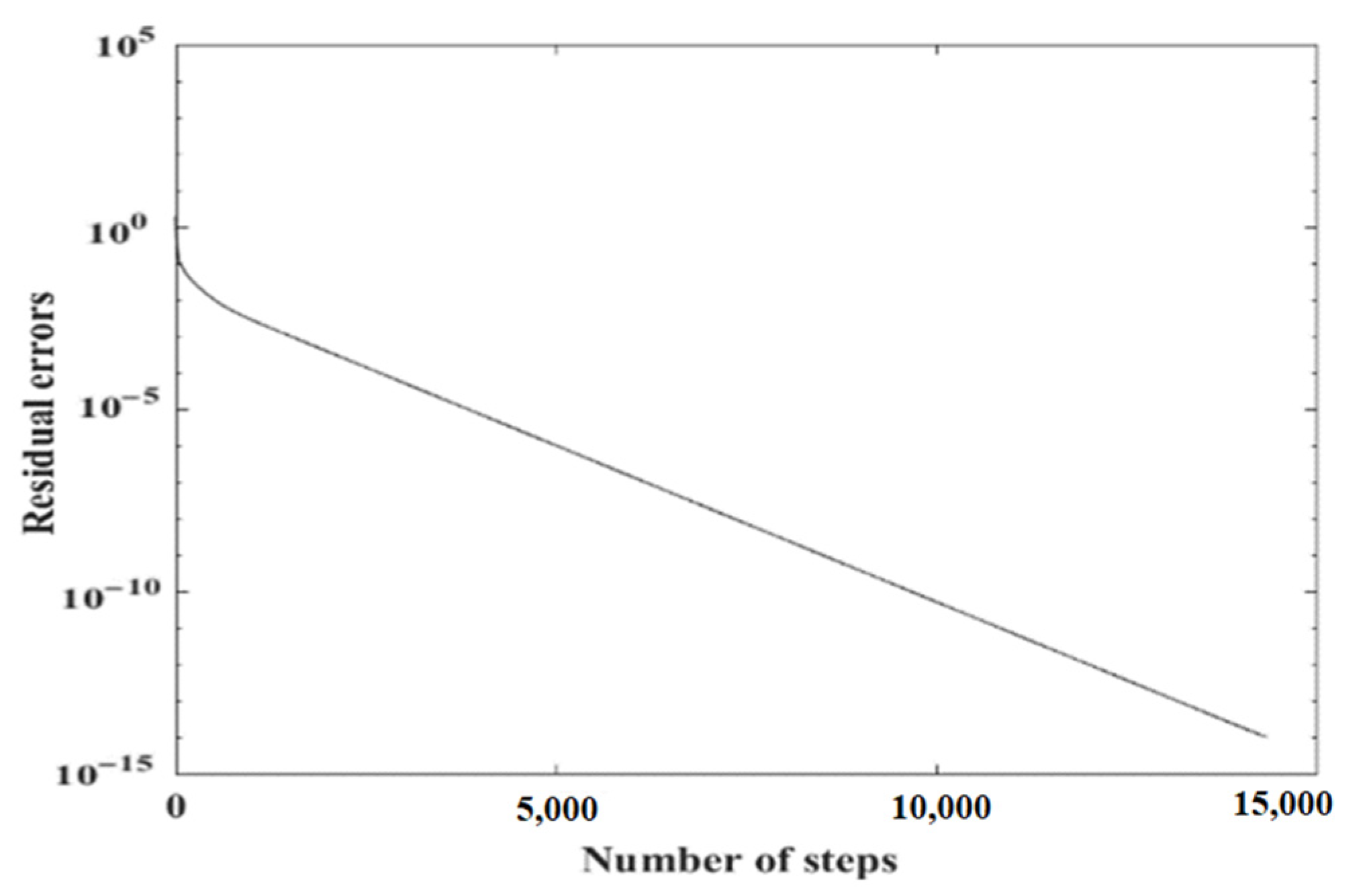
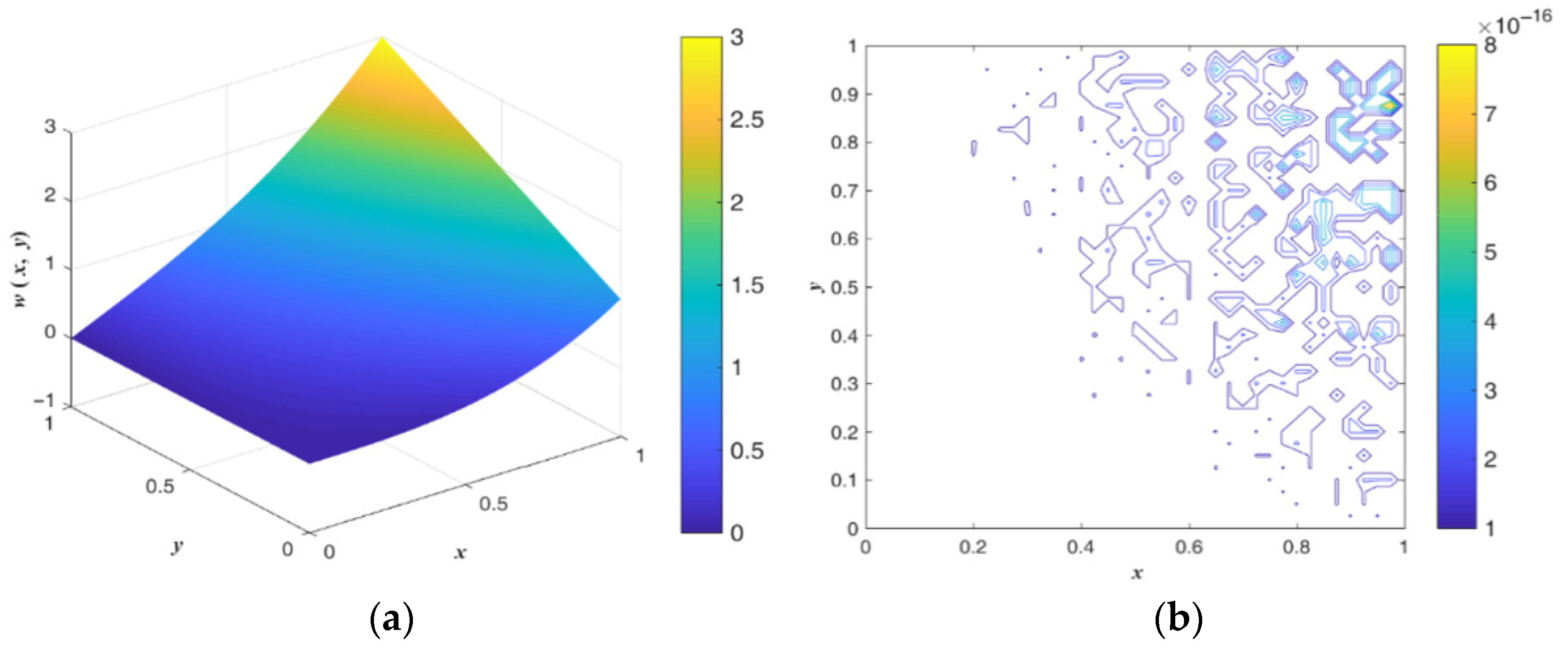
The domain is given by $\mathsf{\Omega } =\left\{\left(x,y\right)|0 \le x \le 1,0 \le y \le 1\right\}$. Here, we set the parameters as $N_x=N_y=41,$ $\Delta \mathsf{\lambda } ={10}^{-300},$ $\epsilon ={10}^{-14},$ $E_{xyz}={10}^4,$ and start from an initial guess value of $w_{i,j}=1$. Figure 7 shows the convergence of residual errors, and the numerical result and absolute errors are shown in Figure 8. The present scheme by the EM converges within $1.4346\times {10}^4$, being better than that established in Chen et al. [26] by RK4, which converges within $5.6944\times {10}^4$ iterations. Figure 8b shows that the maximum error of the numerical solution is smaller than $2.466916\times {10}^{-13}$, which is better than the maximum error of $2.2\times {10}^{-7}$ achieved by Liu [15] and the error of $1.2\times {10}^{-12}$ realized by Chen et al. [26]. Here, we find that the RK4 for the linear Poisson equation has the same order as the EM. That is, the initial guess value is the main reason for numerical accuracy when the convergence angle $S_E$ is small enough.

Figure 7. The convergence plot of Example 2.

Figure 8. Potential distributions for a linear Poisson problem: (a) exact solution; (b) absolute errors.

To verify the initial guess value problem and considering $E_{xyz}={10}^{14},$ the ratio from ${\mathrm{Z}}_{\mathsf{\Gamma }}\left(i,1\right)$ to ${\mathrm{Z}}_{\mathsf{\Gamma }}\left(i,{\mathrm{N}}_y\right)$ is bisected as follows:

$${\mathrm{Z}}_{\mathsf{\Omega }}\left(i,j\right)={\mathrm{Z}}_{\mathsf{\Gamma }}\left(i,1\right)+\left(j-1\right)\frac{{\mathrm{Z}}_{\mathsf{\Gamma }}\left(i,1\right)-{\mathrm{Z}}_{\mathsf{\Gamma }}\left(i,{\mathrm{N}}_y\right)}{{\mathrm{N}}_y},\{\begin{array}{c}i=2,\dots , {\mathrm{N}}_x-1\\ j=2,\dots , {\mathrm{N}}_y-1\end{array}.$$

(17)

The contour of the initial guess value of ${\mathrm{Z}}_{\mathsf{\Omega }}$ is shown in Figure 9. The numerical result and absolute errors are shown in Figure 10. The present scheme by the EM converges within one step, and the maximum error of the numerical solution is smaller than $8.881784\times {10}^{-16}$.

Figure 9. For Example 2: the contour of the initial guess value of ${\mathrm{Z}}_{\mathsf{\Omega }}$.

Figure 10. Potential distributions for a linear Poisson problem: (a) numerical solution; (b) absolute errors.

Further, a two-dimensional nonlinear Poisson equation is tested as follows:

$${\nabla }^{2}w=w^2+6x-x^6-4x^{4}y-4x^2{y}^2.$$

(18)

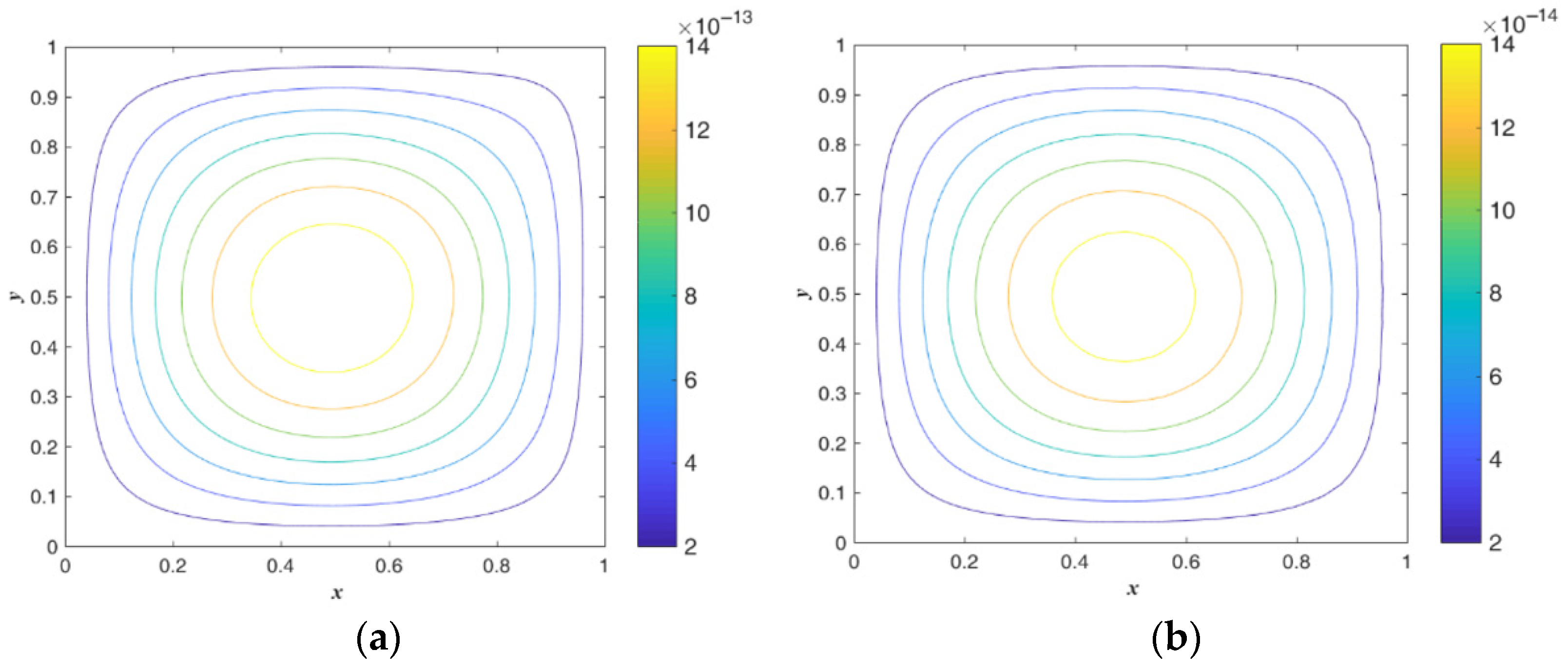
The analytical solution of Equation (18) is the same as Equation (16). To compare our results with Chen et al. [26], the parameters are set as $N_x=N_y=61,$ $E_{xyz}={10}^5,$ and we start from an initial value of $w_{i,j}=1$. For the nonlinear problem, in Chen et al. [26], RK4 and the EM converge to the criteria condition within $1.3686\times {10}^4$ and $1.25972\times {10}^5$ iterations, respectively. Here, we find that the minimum grid for RK4 and the EM is $E_{xyz}={10}^4,$ and $E_{xyz}={10}^5$; that is, as shown in Figure 1, higher-order numerical integration methods allow a large convergence angle, $S_E$, for nonlinear problems. The maximum errors of the numerical solution of the EM and RK4 are $1.578515\times {10}^{-12}$ and $1.529887\times {10}^{-13}$, as shown in Figure 11, which are better than the error of $1.8\times {10}^{-7}$ achieved by Liu [15].

Figure 11. The absolute error distributions for a nonlinear Poisson problem: (a) EM; (b) RK4.

According to Equation (17), the numerical result and absolute errors of the FTIM by the EM are shown in Figure 12 when starting from an initial value of $w^{*}=\max \Vert w_{\mathsf{\Gamma }}\Vert ·{\mathrm{Z}}_{\mathsf{\Omega }}$. The present scheme converges within one step, and the numerical solution’s maximum error is smaller than $8.881784\times {10}^{-16}$. Therefore, linear and nonlinear problems have the same initial guess value, and the nonlinear effect is only shown in the convergence gradient.

Figure 12. Potential distributions for a nonlinear Poisson problem: (a) numerical solution; (b) absolute errors.

3.3. Example 3

According to the literature [2,14], we consider the nonlinear elliptic equation as follows:

$${\nabla }^{2}w+w-0.001w^3=F, 0 \le x \le 1, 0 \le y \le 1.$$

(19)

The analytical solution of Equation (19) is

$$w\left(x,y\right)=-\frac{5}{6}\left(x^3+y^3\right)+3\left(x^{2}y+x{y}^2\right).$$

(20)

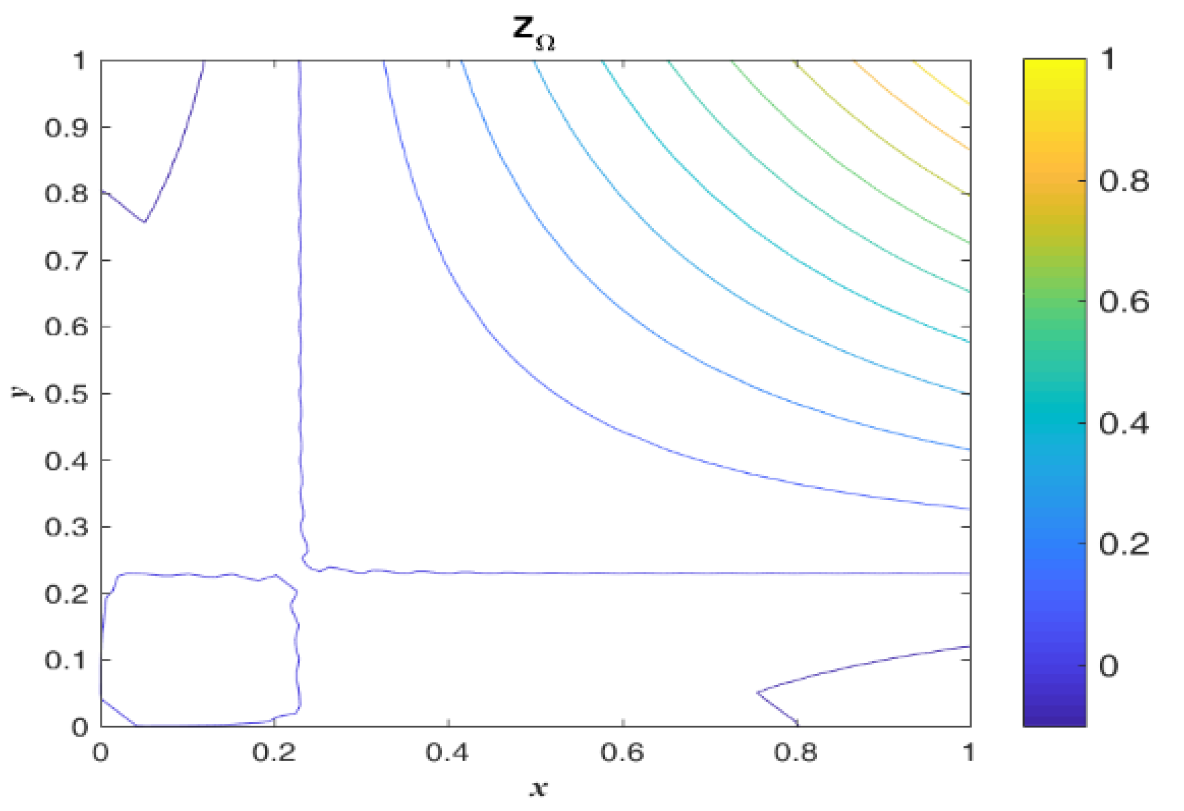
The BCs can be computed exactly by Equation (20). The parameters are set as follows: $N_x=N_y=61,$ $E_{xyz}={10}^5,$ and starting from an initial value of $w^{*}=\max \Vert w_{\mathsf{\Gamma }}\Vert ·{\mathrm{Z}}_{\mathsf{\Omega }}$ according to Equation (15). The contour of the initial guess value of ${\mathrm{Z}}_{\mathsf{\Omega }}$ is shown in Figure 13. The results show that the residual errors are reduced to ${10}^{-14}$ with $1.3514\times {10}^4$ iterations. The numerical results and absolute errors are plotted in Figure 14. The figure shows that the maximum error in the numerical solution is smaller than $5.1059\times {10}^{-13}$, which is better than that of Zhu et al. [2] with ${10}^{-5}$ and Liu and Atluri [14] with $4.4\times {10}^{-5}$. Because the initial guess value cannot be exactly obtained, numerical iteration is inevitable. The results show that the proposed method effectively and accurately solves nonlinear problems.

Figure 13. For Example 3: the contour of the initial guess value of ${\mathrm{Z}}_{\mathsf{\Omega }}$.

Figure 14. Potential distributions for a nonlinear Poisson problem: (a) numerical solution; (b) absolute errors.

3.4. Example 4

According to Ku et al. [16], we consider the three-dimensional nonlinear Helmholtz equation:

$${\nabla }^{2}w=k^2\left(w\right)w, 0 \le x \le 1, 0 \le y \le 1,$$

(21)

where $k^2\left(w\right)$ is assigned as $6w^2$. The analytical solution of Equation (21) is

$$w\left(x,y,z\right)=\frac{1}{x+y+z+1}.$$

(22)

The domain is given by $\mathsf{\Omega } =\left\{\left(x,y,z\right)|0 \le x \le 9,0 \le y \le 9,0 \le z \le 9\right\}$. The parameters used are as follows:$N_x=N_y=N_z=21$ and $E_{xyz}={10}^4.$ For convenience’s sake, the index, such as $i,j,k=1,$ $N_x,N_y$ or $N_z$, is indicated on the BCs. According to the BCs on ${\mathrm{Z}}_{\mathsf{\Gamma }}, \left(x,y,N_Z=1\right)$ is known, the contour of ${\mathrm{Z}}_{\mathsf{\Omega }}$ is shown in Figure 15, and ${\mathrm{Z}}_{\mathsf{\Omega }}$ can be obtained as follows:

$${\mathrm{Z}}_{\mathsf{\Omega }}\left(i,j,k\right)={\mathrm{Z}}_{\mathsf{\Omega }}\left(i-1, j+1, k\right),\{\begin{array}{c}i=2,\dots ,{\mathrm{N}}_x-1\\ j=2,\dots ,{\mathrm{N}}_y-1\\ k=1,\dots ,{\mathrm{N}}_z\end{array}.$$

(23)

Figure 15. For Example 4: the contour of the initial guess value of ${\mathrm{Z}}_{\mathsf{\Omega }}$.

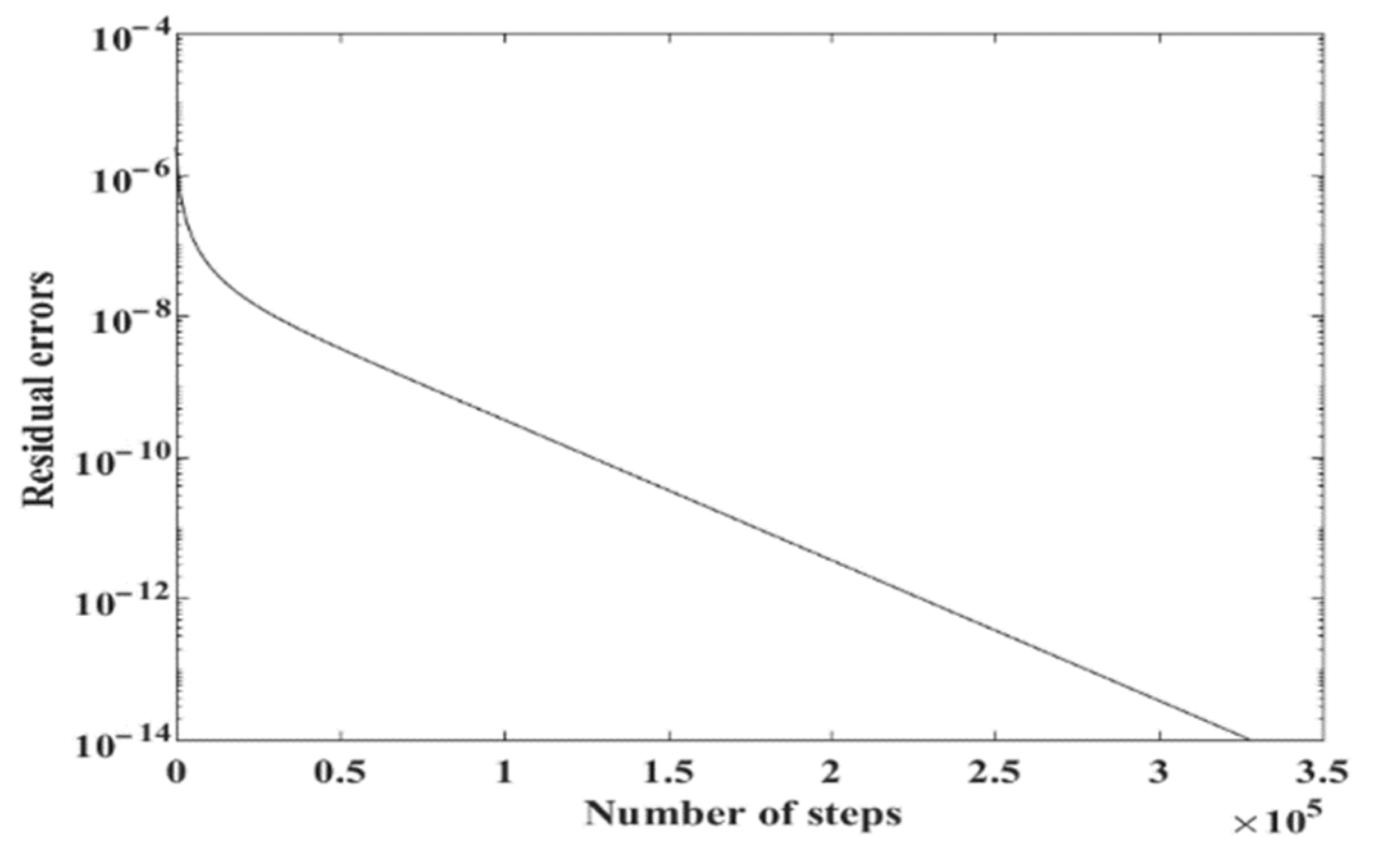
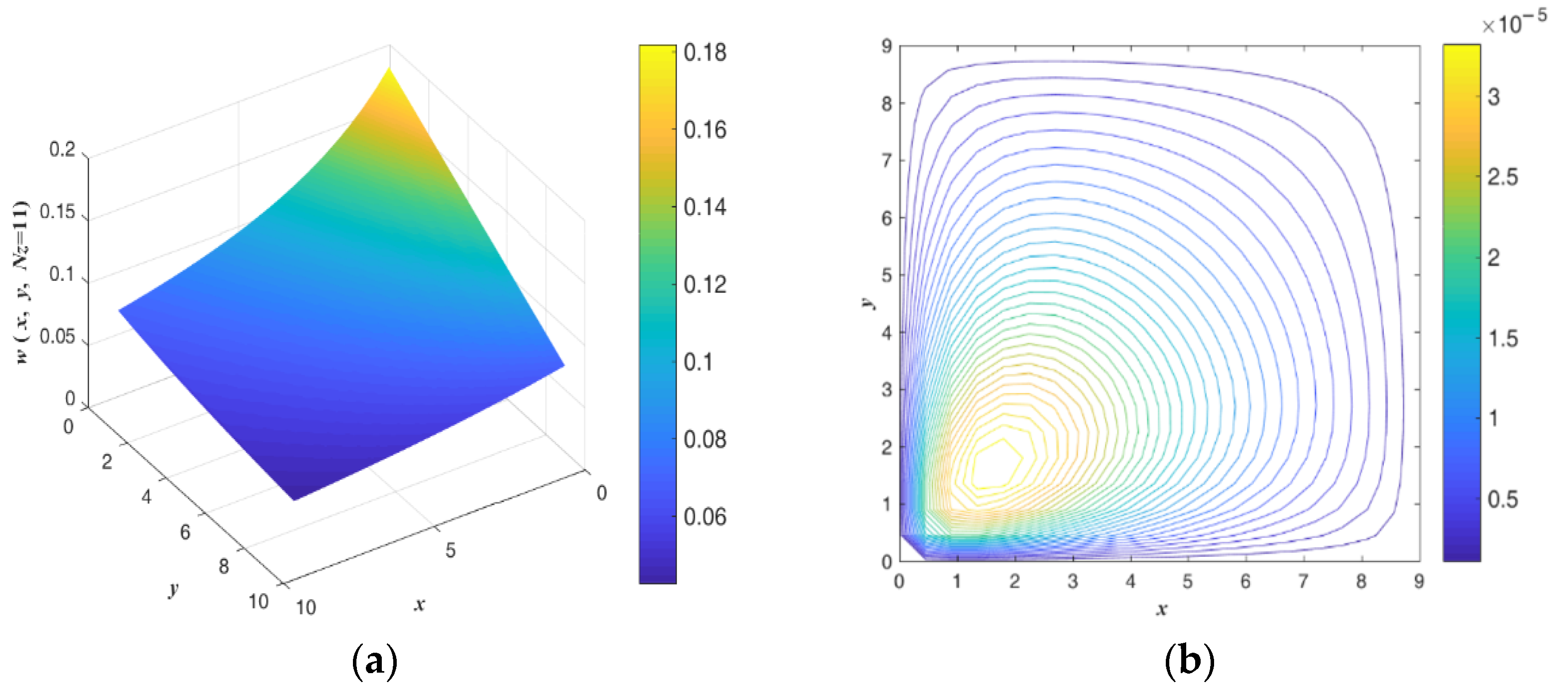
The residual errors are reduced to ${10}^{-14}$ with $3.27761\times {10}^5$ iterations, as shown in Figure 16. The numerical results and absolute errors on the $z=4.5$ plane are plotted in Figure 17. The figure shows that the maximum error of the numerical solution is smaller than $3.432\times {10}^{-5}$. Here, we find that $S_E$ is too large to converge to the true solution, even when using the correct initial guess value.

Figure 16. The convergence plot of Example 4.

Figure 17. Potential distributions for a nonlinear Helmholtz problem: (a) numerical solution; (b) absolute errors.

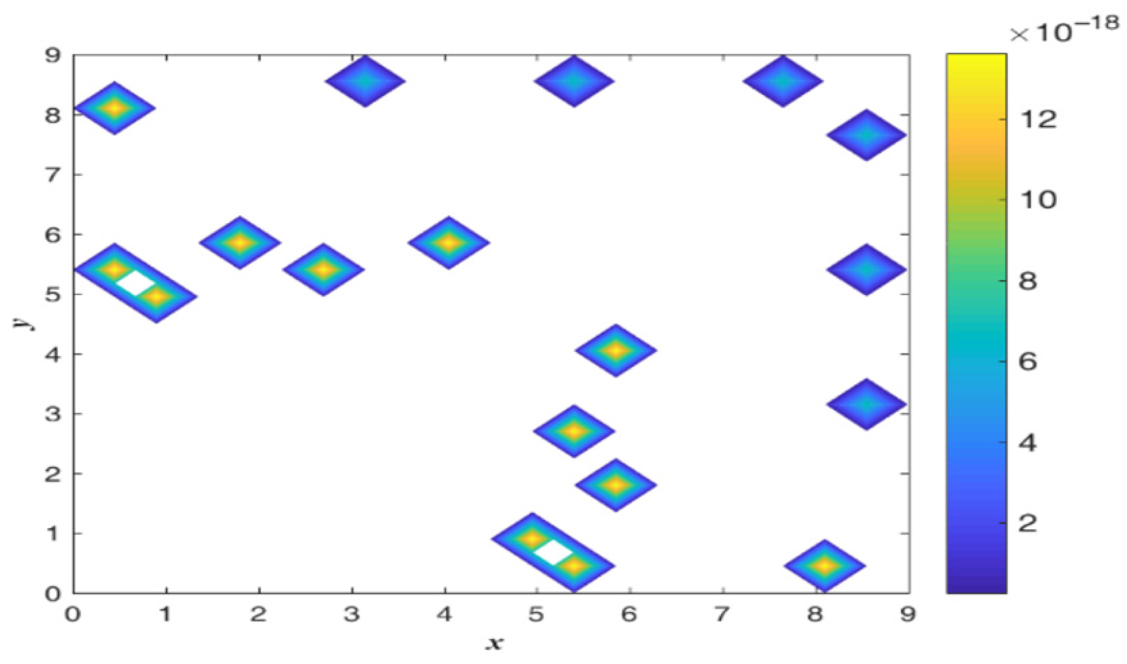
The absolute error is shown in Figure 18 when $E_{xyz}={10}^{14}$ is considered. The present scheme converges within one step, and the maximum error of the numerical solution is smaller than $1.387\times {10}^{-17}$. The numerical results are better than those of Ku et al. [16] with ${10}^{-6}$ and Chen et al. [26] with $8.884\times {10}^{-6}$. Tsai et al. [17] used the method of fundamental solutions with Chebyshev polynomials to solve this problem, and the maximum root mean square error approached $6.54\times {10}^{-12}$. However, Ku et al. [16] and Tsai et al. [17] encountered the same problem, being unable to obtain the correct initial guess value, resulting in a failure to converge. Hence, these results demonstrate the efficiency and accuracy of the proposed scheme for solving the three-dimensional nonlinear Helmholtz equation.

Figure 18. The absolute error distributions for a nonlinear Helmholtz problem under $E_{xyz}={10}^{14}$.

4. Conclusions

In this paper, we have successfully introduced a normalized boundary solution and constructed a straightforward numerical procedure based on the constraint-type FTIM to solve multi-dimensional nonlinear elliptic-type PDEs. All parameters of the constrain-type FTIM, the viscosity-damping coefficient, system energy (the discrete number of grids) and minimum fictitious time size, were combined into a space-time constraint coefficient, so numerical accuracy and computational efficiency depend on the initial condition. According to the two-point solution of a nonlinear dynamic system from the Lie-group shooting method, the normalized boundary solution of elliptic-type PDEs can be constructed from the boundary conditions to avoid the problem of the initial guess value. Several nonlinear numerical examples are tested, and it is astounding that a two-point boundary value solution can satisfy the stringent convergent criterion. Even under a very small fictitious time step, it can quickly approach the exact solution within one step. Until now, there has been no evidence that the numerical methods can be applied to calculate multi-dimensional nonlinear elliptic-type PDEs in one step. Hence, it can be concluded that the proposed numerical procedure is highly accurate, stable, effective and insensitive to the discrete number of grids. Future works could focus on extending the constraint-type FTIM to solve backward-in-time parabolic, hyperbolic and parabolic–hyperbolic types of nonlinear PDEs.

References

- Atluri, S.N.; Zhu, T. A new meshless local Petrov-Galerkin (MLPG) approach in computational mechanics. Comput. Mech. 1998, 22, 117–127. [Google Scholar] [CrossRef]
- Zhu, T.; Zhang, J.; Atluri, S.N. A meshless local boundary integral equation (LBIE) method for solving nonlinear problems. Comput. Mech. 1998, 22, 174–186. [Google Scholar] [CrossRef]
- Cheng, A.H.D.; Golberg, M.A.; Kansa, E.J.; Zammito, G. Exponential convergence and H-c multiquadric collocation method for partial differential equations. Numer. Meth. Part Differ. Equ. 2003, 19, 571–594. [Google Scholar] [CrossRef]
- Cho, H.A.; Golberg, M.A.; Muleshkov, A.S.; Li, X. Trefftz methods for time dependent partial differential equations. Comput. Mat. Cont. 2004, 1, 1–38. [Google Scholar]
- Jin, B. A meshless method for the Laplace and biharmonic equations subjected to noisy boundary data. CMES-Comput. Model. Engrg. Sci. 2004, 6, 253–262. [Google Scholar]
- Hu, H.Y.; Li, Z.C.; Cheng, A.H.D. Radial basis collocation methods for elliptic boundary value problems. Comput. Math. Appl. 2005, 50, 289–320. [Google Scholar] [CrossRef]
- Hu, H.Y.; Chen, J.S. Radial basis collocation method and quasi-Newton iteration for nonlinear elliptic problems. Numer. Meth. Part Differ. Equ. 2008, 24, 991–1017. [Google Scholar] [CrossRef]
- Fan, C.M.; Li, H.H.; Kuo, C.L. The modified collocation Trefftz method and Laplacian decomposition for solving two-dimensional Stokes problems. J. Mar. Sci. Technol.-Taiwan 2011, 19, 522–530. [Google Scholar] [CrossRef]
- Zhang, X.H.; Ouyang, J.; Zhang, L. Element-free characteristic Galerkin method for Burgers’ equation. Eng. Anal. Bound. Elem. 2009, 33, 356–362. [Google Scholar] [CrossRef]
- Seydaoğlu, M. A meshless method for Burgers’ equation using multiquadric radial basis functions with a Lie-group integrator. Mathematics 2019, 7, 113. [Google Scholar] [CrossRef]
- Milewski, S. Combination of the meshless finite difference approach with the Monte Carlo random walk technique for solution of elliptic problems. Comput. Math. Appl. 2018, 76, 854–876. [Google Scholar] [CrossRef]
- Colbrook, M.J.; Flyer, N.; Fornberg, B. On the Fokas method for the solution of elliptic problems in both convex and non-convex polygonal domains. J. Comput. Phys. 2018, 374, 996–1016. [Google Scholar] [CrossRef]
- Ezeh, I.P.; Kamoh, N.M. On the numerical solution of second order two-dimensional Laplace equations using the alternating-direction implicit method. J. Phys. Commun. 2020, 4, 105004. [Google Scholar] [CrossRef]
- Liu, C.S.; Atluri, S.N. A novel time integration method for solving a large system of non-linear algebraic equations. CMES-Comp. Model. Eng. Sci. 2008, 31, 71–83. [Google Scholar]
- Liu, C.S. A fictitious time integration method for two-dimensional quasilinear elliptic boundary value problems. CMES-Comp. Model. Eng. Sci. 2008, 33, 179–198. [Google Scholar]
- Ku, C.Y.; Yeih, W.C.; Liu, C.S.; Chi, C.C. Applications of the fictitious time integration method using a new time-like function. CMES-Comp. Model. Eng. Sci. 2009, 43, 173–190. [Google Scholar]
- Tsai, C.C.; Liu, C.S.; Yeih, W.C. Fictitious time integration method of fundamental solutions with Chebyshev polynomials for solving Poisson-type nonlinear PDEs. CMES-Comp. Model. Eng. Sci. 2010, 56, 131–151. [Google Scholar]
- Chang, C.W. A fictitious time integration method for multi-dimensional backward heat conduction problems. CMES-Comp. Model. Eng. Sci. 2010, 19, 285–314. [Google Scholar]
- Ku, C.Y.; Yeih, W.C.; Liu, C.S. Solving non-linear algebraic equations by a scalar Newton-homotopy continuation method. Int. J. Nonlinear Sci. Numer. Simul. 2010, 11, 435–450. [Google Scholar] [CrossRef]
- Liu, C.S.; Atluri, S.N. Simple “residual-norm” based algorithms, for the solution of a large system of non-linear algebraic equations, which converge faster than the Newton’s method. CMES-Comp. Model. Eng. Sci. 2011, 71, 279–304. [Google Scholar] [CrossRef]
- Chen, Y.W.; Chang, C.M.; Liu, C.S.; Chang, J.R. Application of a manifold-based exponentially convergent algorithm to solve elliptic boundary-value problems. IMA J. Numer. Anal. 2014, 34, 362–389. [Google Scholar] [CrossRef]
- Ku, C.Y.; Kuo, C.L.; Fan, C.M.; Liu, C.S.; Guan, P.C. Numerical solution of three-dimensional Laplacian problems using the multiple scale Trefftz method. Eng. Anal. Bound. Elem. 2015, 50, 157–168. [Google Scholar] [CrossRef]
- Chen, Y.W. High order implicit and explicit Lie-group schemes for solving backward heat conduction problems. Int. J. Heat Mass Transf. 2016, 101, 1016–1029. [Google Scholar] [CrossRef]
- Chen, Y.W. A highly accurate backward-forward algorithm for multi-dimensional backward heat conduction problems in fictitious time domains. Int. J. Heat Mass Transf. 2018, 120, 499–514. [Google Scholar] [CrossRef]
- Chen, Y.W. Simultaneous determination of the heat source and the initial data by using an explicit Lie-group shooting method. Numer. Heat Tranf. B-Fundam. 2019, 75, 239–264. [Google Scholar] [CrossRef]
- Chen, Y.W.; Liu, C.S.; Chang, Y.S.; Chang, J.R. Constraint type fictitious time integration method to solve non-linear multi-dimensional elliptic partial differential equations. J. Mar. Sci. Technol.-Taiwan 2020, 28, 168–178. [Google Scholar] [CrossRef]
- Chang, Y.S.; Chen, Y.W.; Liu, C.S.; Chang, J.R. A non-iteration solution for solving the backward-in-time two-dimensional Burgers’ equation with a large Reynolds number. J. Mar. Sci. Technol.-Taiwan 2022, 30, 75–85. [Google Scholar] [CrossRef]
Disclaimer/Publisher’s Note: The statements, opinions and data contained in all publications are solely those of the individual author(s) and contributor(s) and not of MDPI and/or the editor(s). MDPI and/or the editor(s) disclaim responsibility for any injury to people or property resulting from any ideas, methods, instructions or products referred to in the content. |
© 2023 by the authors. Licensee MDPI, Basel, Switzerland. This article is an open access article distributed under the terms and conditions of the Creative Commons Attribution (CC BY) license (https://creativecommons.org/licenses/by/4.0/).