Constructing Exact and Approximate Diffusion Wave Solutions for a Quasilinear Parabolic Equation with Power Nonlinearities

Abstract

The paper studies a degenerate nonlinear parabolic equation containing a convective term and a source (reaction) term. It considers the construction of approximate solutions to this equation with a specified law of diffusion wave motion, the existence of these solutions being proved in our previous studies. A stepwise algorithm of the numerical solution with a time-difference scheme is proposed, the second-order difference scheme being used in such problems for the first time. At each step the problem is solved iteratively on the basis of a radial basis function (RBF) collocation method. In order to verify the numerical solution algorithm, two classes of exact generalized traveling wave solutions are proposed, whose construction is reduced to solving a Cauchy problem for second order ordinary differential equations (ODEs) with a singularity at the higher derivative. The theorem of the existence and uniqueness of the analytical solution in the form of a power series is proved for it, and the estimates of the radius of convergence are obtained. The Euler method is used to prove a similar statement concerning the existence of a continuous solution in the non-analytical case. The RBF collocation method is also applied for the approximate solution of the Cauchy problem. The solutions to the Cauchy problem are numerically analyzed, and this has enabled us to reveal and describe some of their properties, including those not previously observed, and to assess the accuracy of the method.

1. Introduction

This paper deals with the construction and study of one special class of solutions to second-order nonlinear parabolic evolution equations. Thus we consider an equation of the following form:

$$T_t={\left({\Phi }_1\left(T\right)\right)}_{xx}+{\left({\Phi }_2\left(T\right)\right)}_x+{\Phi }_3\left(T\right).$$

(1)

Here, $t,x$ are independent variables: t is time, x is a spatial variable, $T(t,x)$ is the required function, ${\Phi }_i,i=1,2,3$ are given functions. The particular cases of Equation (1) are represented by such widely known models of continuum mechanics as the porous medium equation and its generalizations, as well as the convection-diffusion equation [1].

For equations of this form, a special class of solutions termed diffusion (heat, filtration) waves, describing disturbances propagating along the zero (resting) background at a finite velocity, is of great interest [2]. A diffusion wave consists of two solutions, non-negative and trivial, which are continuously joined by a certain curve that is called the wave front (zero front). Such solutions are both of mathematical interest, since they are inherent to hyperbolic equations and systems rather than parabolic ones [3], and of applied interest, since they describe specific processes in physical and biological systems, particularly, filtration of fluids in porous media [4], processes in high-temperature plasma [5], and evolution of biological populations [6]. Nonlinear parabolic equations and systems have some other applications; however, formulations without degeneration are usually considered [7,8].

Unfortunately, the science of today does not know how to find general solutions to nonlinear equations of mathematical physics similar to (1). In this connection, researchers face three main questions: Does a solution exist and is it unique? How can an approximate solution be found? How can the correctness of the found approximate solution be verified?

Existence theorems generally imply the specification of initial and boundary conditions. Earlier we proved a number of statements of the existence and uniqueness of diffusion wave type solutions for various forms of Equation (1) and at various boundary conditions. Two main types of boundary conditions were considered: when (a) the diffusion wave front is known [9,10] and (b) the boundary conditions generating a diffusion wave are given [11,12].

To solve such problems approximately in various particular cases, we previously [13,14,15] developed algorithms based on the boundary element method (BEM) [16] and the dual reciprocity method (DRM) [17,18,19,20] with a time difference approximation. The DRM is based on approximation using radial basis functions (RBF) [21,22], which have been widely used for solving differential equations in recent decades. This approach can be applied both in the case of one spatial variable and for two spatial variables, see [14,15], where the generalized porous medium equation is studied. In this paper, to solve the boundary value problems numerically, we use an RBF collocation method (RBFCM), which is simpler when applied to one-dimensional problems.

As applied to solving elliptic problems, two most widespread methods of this kind should be noted. The Kansa method and its modifications [23,24] imply the representation of the required function as a linear combination of some RBFs and the determination of the coefficients by satisfying the equation at the collocation points inside the solution domain and satisfying the boundary conditions at the collocation points on the domain boundary. This method is mostly applicable to linear problems. The method of particular solutions is commonly used for nonlinear equations [25,26]. It consists of the representation of the problem solution as a sum of a particular solution of the original inhomogeneous equation and the solution of the corresponding homogeneous equation. The particular solution is found by inhomogeneity expansion in terms of RBFs; the expansion coefficients are determined by satisfying the equation at the internal and boundary collocation points. The homogeneous equation with boundary conditions recalculated in view of the found particular solution can be solved by the BEM, by the method of fundamental solution [27,28] or by another method. Reviews of different methods using RBFs can be found in [22,29,30].

Time–space RBFs can be used for solving parabolic problems [31], yet a parabolic equation is generally represented as elliptic, and an implicit or explicit time step scheme is used [19,32,33]. In our previous studies [13,14,15] the time derivative was transferred to the right-hand side of the Poisson equation and computed by a first-order finite difference formula. At each time step an elliptic problem can be solved by one of the above RBF collocation methods.

Finally, for checking the correctness of the solution under appropriate conditions when it is very rarely possible to prove any rigorous mathematical statements about the convergence of approximate methods, the challenges of verifying the calculation results become especially urgent. One of the most widespread ways of solving this challenge and describing laboratory experiments [34] is using exact solutions [35] whose construction is generally reducible to the analytical or, more often, numerical integration of ordinary differential equations. These equations often are the so-called Li$\acute{e}$nard equations [36]. For equations such as (1) in various particular modifications, including the porous medium equation [37], the generalized porous medium equation [9] and its extensions, as well as the convection-diffusion equation [10], we proposed new classes of exact solutions having a diffusion wave type. Besides, the test calculations can be made by power series [38], which are constructed as solutions in the proof of theorems of existence in the class of analytical functions if these series are considered in the domain of convergence. This approach termed the method of power series (MPS) is often applied in order to disclose singularities for constructing local solutions of equations of mathematical physics [39].

The main content of this paper, which continues our earlier studies, is the development of algorithmic tools for constructing approximate solutions of the required form. We develop and verify an approximate method based, as was noted, on RBF expansion and on the collocation method and apply it to numerical analysis. This method is adapted and applied to solving the degenerate Equation (1) for the first time. Moreover, we do not know any other approach for the nonlocal numerical solution of the problem under consideration. Besides, we fill some gaps in the study of exact solutions. Particularly, we obtain estimates for the series convergence radii, this being critical for using the truncated series in the verification of the RBFCM calculation results obtained by the RBF collocation method. Finally, for the case of a simple travelling wave, we have managed to refuse from the analyticity requirement, which essentially restricts the generality of consideration, due to using the Euler method with the aim to prove the existence of the solution. This significantly generalizes the result obtained earlier in [12].

2. Problem Formulation

Provided the functions ${\Phi }_1\left(T\right),{\Phi }_2\left(T\right)$ are differentiable, Equation (1) can be rewritten as:

$$T_t={\left({\Phi }_1^{\prime }\left(T\right)T_x\right)}_x+{\Phi }_2^{\prime }\left(T\right)T_x+{\Phi }_3\left(T\right).$$

(2)

Consider the case of the power functions ${\Phi }_i\left(T\right),i=1,2,3$, which is most commonly encountered in the literature [1] since it is the closest to applications. Thus, suppose:

$${\Phi }_1^{\prime }\left(T\right)={\lambda }_1{T}^{{\sigma }_1},{\Phi }_2^{\prime }\left(T\right)={\lambda }_2{T}^{{\sigma }_2},{\Phi }_3\left(T\right)={\lambda }_3{T}^{{\sigma }_3},$$

where ${\sigma }_i,i=1,2,3$ are positive constants, ${\sigma }_1+{\sigma }_3>1$, ${\lambda }_i,i=1,2,3$, are constants, ${\lambda }_1>0$.

We make the following substitution of the required function: $u={\Phi }_1^{\prime }\left(T\right)={\lambda }_1{T}^{{\sigma }_1}.$ After simple transformations, Equation (2) becomes:

$$u_t=u{u}_{xx}+\frac{1}{\sigma }{u}_x^2+A{u}^{\theta }{u}_x+B{u}^{\beta }.$$

(3)

Here, $\sigma ={\sigma }_1>0$, $\theta ={\sigma }_1/{\sigma }_2>0$, $\beta ={\sigma }_3/{\sigma }_1+1-1/{\sigma }_1>0$, $A={\lambda }_2{\lambda }_1^{-1/\sigma },$$B={\lambda }_3{\lambda }_1^{1/\sigma -1/{\sigma }_3}$.

For Equation (3), we consider the boundary condition which specifies the diffusion wave front:

$${u(t,x)|}_{x=a\left(t\right)}=0,$$

(4)

the function $a\left(t\right)$ must be fairly smooth herewith.

Note that problem (3), (4) is satisfied by the function $u\equiv 0$. However, the uniqueness of the solution is violated in this case, and there can be a nonzero solution as well. Thus, earlier [10] we proved the existence of a nontrivial analytical solution to problem (3), (4).

3. RBFCM Solution

The analytical solution in the form of a series, whose existence was proved in [10], is meaningful in the vicinity of the given front of a diffusion wave with a generally unknown radius. Therefore, it is relevant to construct a numerical solution to problem (3), (4) on a given finite time interval. This is what is discussed in this section; herewith, the important feature that distinguishes this paper from our previous ones is the application of the RBFCM instead of the BEM, and this simplifies the algorithm in the one-dimensional case.

The analysis of the methods, the nonlinear form of Equation (3), and the nonclassical form of the boundary condition (4) give grounds for solving problem (3), (4) at each time step by the method of particular solutions as follows.

We divide the time interval in which problem (3), (4) is to be solved into h-sized steps. At each step, $t_k=kh$, we solve the following boundary value problem for the Poisson equation, which corresponds to (3) and (4) at the moment $t_k$,

$$u_{xx}=\frac{1}{u}\left[u_t-\frac{1}{\sigma }{u}_x^2-A{u}^{\theta }{u}_x-B{u}^{\beta }\right],x\in [0,L),$$

(5)

$${u|}_{x=L}=0,$$

(6)

where $L=a\left(t_k\right)$. It is noted above that problem (3), (4) has a unique nontrivial solution. Therefore, the singularity in the right-hand side of (5) is removable, i.e., the limit of the right-hand side (5) when $x\to L,u\to 0$ exists and is finite.

It can be shown [40] that the following condition follows from the condition (6)

$$\frac{\partial u}{\partial x}{|}_{x=L}=-\sigma \frac{da\left(t_k\right)}{dt}.$$

(7)

The solution of the problem (5)–(7) is constructed as the following sum:

$$u(t_k,x)=U_p\left(x\right)+U_h\left(x\right),$$

(8)

where $U_p\left(x\right)$ is a particular solution to Equation (5) at the moment $t_k$, $U_h\left(x\right)$ is the solution to the following problem for the homogeneous equation:

$$\frac{d^2{U}_h}{d{x}^2}=0,$$

(9)

$$U_h{|}_{x=L}=-U_p\left(L\right),$$

(10)

$$\frac{d{U}_h}{dx}{|}_{x=L}=-\sigma \frac{da\left(t_k\right)}{dt}-\frac{d{U}_p\left(L\right)}{dx}.$$

(11)

Note that, with the found $U_p\left(x\right)$, the solution of problem (9)–(11) is determined uniquely, and this is one thing that governs the choice of the solution method.

Since the right-hand side of Equation (5) depends on the required function and its derivatives, the solution is constructed iteratively according to the following procedure:

$$U_p^{\left(0\right)}\equiv 0,$$

(12)

$$U_h^{\left(n\right)}=-\left(\sigma \frac{da\left(t_k\right)}{dt}+\frac{d{U}_p\left(L\right)}{dx}\right)x-U_p^{\left(n\right)}\left(L\right),$$

(13)

$$\frac{d^2{U}_p^{(n+1)}}{d{x}^2}=g\left(u^{\left(n\right)},\frac{\partial u^{\left(n\right)}}{\partial t},\frac{\partial u^{\left(n\right)}}{\partial x}\right),$$

(14)

where $U_p^{\left(n\right)}$, $U_h^{\left(n\right)}$ and $u^{\left(n\right)}=U_p^{\left(n\right)}+U_h^{\left(n\right)}$ are the n-th iterations of the solutions,

$$g\left(u^{\left(n\right)},\frac{\partial u^{\left(n\right)}}{\partial t},\frac{\partial u^{\left(n\right)}}{\partial x}\right)=\frac{1}{u^{\left(n\right)}}\left[\frac{\partial u^{\left(n\right)}}{\partial t}-\frac{1}{\sigma }{\left(\frac{\partial u^{\left(n\right)}}{\partial x}\right)}^2-A{\left(u^{\left(n\right)}\right)}^{\theta }\frac{\partial u^{\left(n\right)}}{\partial x}-B{\left(u^{\left(n\right)}\right)}^{\beta }\right].$$

To solve Equation (14), we use the expansion of the right-hand side in RBFs,

$$g\left(u^{\left(n\right)},\frac{\partial u^{\left(n\right)}}{\partial t},\frac{\partial u^{\left(n\right)}}{\partial x}\right)=\sum _{i=1}^m{\alpha }_i^{(n+1)}{f}_i\left(x\right).$$

(15)

Here, $f_i\left(x\right)=f_i\left(|x-x_i|\right)$ are RBFs, $x_1,x_2,\dots ,x_m$ are the collocation points belonging to the interval $[0,L)$. For each function $f_i\left(x\right)$ there is such a function ${\widehat{u}}_i$ that $f_i=d^2\widehat{u_i}/d{x}^2$. The coefficients ${\alpha }_i^{(n+1)},i=1,\dots ,m$, are determined from the system of linear algebraic equations:

$$g\left(u^{\left(n\right)},\frac{\partial u^{\left(n\right)}}{\partial t},\frac{\partial u^{\left(n\right)}}{\partial x}\right){|}_{x=x_j}=\sum _{i=1}^m{\alpha }_i^{(n+1)}{f}_i\left(x_j\right),j=1,\dots ,m.$$

(16)

The obtained coefficients will determine the $(n+1)$-th iteration of the particular solution,

$$U_p^{(n+1)}\left(x\right)=\sum _{i=1}^m{\alpha }_i^{(n+1)}{\widehat{u}}_i\left(x\right).$$

(17)

The time derivative is calculated by the finite difference method. In the majority of studies, including ours, there is linear time approximation. In our case the following scheme is used:

$$\frac{\partial u^{\left(n\right)}\left(x_j\right)}{\partial t}=\left\{\begin{array}{cc}\hfill \frac{u^{\left(n\right)}\left(x_j\right)-u(t_{k-1},x_j)}{h},\hfill & \hfill x_j\le a\left(t_{k-1}\right),\hfill \\ \hfill \frac{u^{\left(n\right)}\left(x_j\right)}{h_k^{\left(j\right)}},\hfill & \hfill x_j>a\left(t_{k-1}\right),\hfill \end{array}\right.$$

(18)

where $h_k^{\left(j\right)}=t_k-t^{\left(j\right)}$, $t^{\left(j\right)}=a^{-1}\left(x_j\right)$, $t=a^{-1}\left(x\right)$ is the function inverse to $x=a\left(t\right)$. Thus, $t^{\left(j\right)}$ is the time instant that the diffusion wave front is at the point $x_j$.

In this study, to increase the calculation accuracy, we use quadratic time approximation. To do this, we make the following computations. Having taken a total time derivative in the condition (4), when $x=a\left(t\right)$, we obtain:

$$\frac{\partial u}{\partial t}=-\frac{\partial u}{\partial x}\frac{da}{dt}.$$

(19)

Substitution of (19) into Equation (3) gives the equality:

$$\frac{\partial u}{\partial x}=-\sigma \frac{da}{dt},$$

(20)

which in particular results in the condition (7). Substituting (20) into (19), we have:

$$\frac{\partial u}{\partial t}{|}_{x=a\left(t\right)}=\sigma {\left(\frac{da}{dt}\right)}^2.$$

(21)

Thus, the conditions of the original problem allow us to find the value of the time derivative of the required function at the diffusion wave front. This enables the time derivative in system (16) to be computed under the assumption of quadratic approximation as follows:

$$\frac{\partial u^{\left(n\right)}\left(x_j\right)}{\partial t}=\left\{\begin{array}{cc}\frac{u(t_{k-2},x_j)-4u(t_{k-1},x_j)+3u^{\left(n\right)}\left(x_j\right)}{2h},\hfill & x_j\le a\left(t_{k-2}\right),\hfill \\ \frac{1}{h}\left(\frac{2h+h_j^{(k-1)}}{h+h_{k-1}^{\left(j\right)}}{u}^{\left(n\right)}\left(x_j\right)-\frac{h+h_j^{(k-1)}}{h_{k-1}^{\left(j\right)}}u(t_{k-1},x_j)\right),\hfill & a\left(t_{k-2}\right)<x_j\le a\left(t_{k-1}\right),\hfill \\ \frac{2u^{\left(n\right)}\left(x_j\right)-\sigma {\left[a^{\prime }\left(t^{\left(j\right)}\right)\right]}^2{h}_k^{\left(j\right)}}{h_k^{\left(j\right)}},\hfill & x_j>a\left(t_{k-1}\right).\hfill \end{array}\right.$$

(22)

The first line in the right-hand side of Equation (22) is the three-point finite difference formula on the uniform mesh (as for the point $x_1$ in Figure 1); the second line is the three-point finite difference formula on the nonuniform mesh (point $x_2$ in Figure 1); the third line is the two-point formula for the case when the values of both the function and its derivative are specified at one of the points (point $x_3$ in Figure 1).

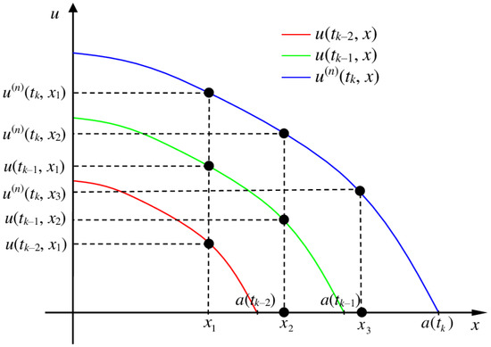
Figure 1. To the calculation of the time derivative: $x_1\le a\left(t_{k-2}\right);a\left(t_{k-2}\right)<x_2\le a\left(t_{k-1}\right);x_3>a\left(t_{k-1}\right)$.

The iteration processes (12)–(22) stop if

$$\frac{|u^{\left(n\right)}\left(0\right)-u^{(n-1)}\left(0\right)|}{|u^{\left(n\right)}\left(0\right)|}<\epsilon ,$$

where $\epsilon >0$ is the specified accuracy. Then the following function continuous in x is taken as a solution to problem (3), (4) in the step $t=t_k$:

$$u(t_k,x)=U_p^{\left(n\right)}\left(x\right)+U_h^{\left(n\right)}\left(x\right).$$

(23)

4. Analytical Construction of Exact Solution

Verification of numerical solutions requires the availability of a fairly general class of exact solutions to problem (3), (4). Let us further investigate the issue of seeking nontrivial exact solutions, whose construction is reduced to the integration of Cauchy problems for ODEs. We studied this problem earlier in detail for the case of a nonlinear heat conduction equation [37] with a source term [9], which corresponds to the case $A=0$, and we found and investigated new classes of solutions of the form under study. Besides, some exact solutions to problem (3), (4) were obtained in [10] and studied in detail for one particular case in [12]. Note that, besides verification of approximate solutions, exact solutions can be used for the qualitative and numerical analysis of the properties of the problem under study. Travelling waves, simple and generalized, are the simplest and most natural form of exact solutions [41,42]. In what follows, we will seek solutions of this form and study them analytically.

4.1. Reduction to ODEs

We assume that $z=x-a\left(t\right)$ and substitute $u=\psi \left(t\right)v\left(z\right)$ in Equation (3). Having collected the terms and divided by ${\psi }^2\left(t\right)$, we have:

$$v{v}^{″}+\frac{1}{\sigma }{\left(v^{\prime }\right)}^2+A{\psi }^{\theta -1}\left(t\right)v^{\theta }{v}^{\prime }+B{\psi }^{\beta -2}\left(t\right)v^{\beta }+\frac{a^{\prime }\left(t\right)}{\psi \left(t\right)}{v}^{\prime }-\frac{{\psi }^{\prime }\left(t\right)}{{\psi }^2\left(t\right)}v=0.$$

(24)

For Equation (24) to become an ODE with respect to $v\left(z\right)$, it is necessary and enough that the following identical equalities should be fulfilled:

$$\frac{a^{\prime }\left(t\right)}{\psi \left(t\right)}=\mathrm{const},\frac{{\psi }^{\prime }\left(t\right)}{{\psi }^2\left(t\right)}=\mathrm{const},{\psi }^{\theta -1}\left(t\right)=\mathrm{const},{\psi }^{\beta -2}\left(t\right)=\mathrm{const}.$$

(25)

The first two conditions in Equation (25) are a system of two ODEs with two unknown functions, and the last two have the nature of additional consistency conditions which can be satisfied, e.g., by selecting $\theta$ and $\beta$.

Consider successively two possible cases.

1.

Assume that $\psi \left(t\right)=\psi =\mathrm{const}$. It can be assumed without loss of generality that $\psi =1$. Then $a\left(t\right)=\mu t+\eta ,$ where $\mu ,\eta$ are constants, Equation (24) acquires the form of the following ODE:

$$v{v}^{″}+\frac{1}{\sigma }{\left(v^{\prime }\right)}^2+(A{v}^{\theta }+\mu )v^{\prime }+B{v}^{\beta }=0.$$

(26)

We consider in what follows that $\eta =0,\mu >0$, which also preserves the generality of consideration. Equation (26) describes solutions of the simple travelling wave type.

2.

Assume now that $\psi \left(t\right)\ne \mathrm{const}$. Then, it follows from the first two equations in (25) that $\psi \left(t\right)=\omega /(\mu t+\eta ),$$a\left(t\right)=\omega ln(\mu t+\eta )$, where $\mu ,\eta ,\omega$ are nonzero constants, $\eta >0$, i.e., ${(\mu t+\eta )|}_{t=0}>0$. It can be seen that, in this case, the necessary and sufficient condition for the third and fourth equalities in Equation (25) to be fulfilled are the conditions $\theta =1$ and $\beta =2$. Then Equation (24) acquires the form of the following ODE:

$$v{v}^{″}+\frac{1}{\sigma }{\left(v^{\prime }\right)}^2+(Av+\mu )v^{\prime }+B{v}^2+\frac{\mu }{\omega }v=0.$$

(27)

Equation (27) describes solutions of the type of a generalized travelling wave type with a logarithmic front.

The condition (4) at the diffusion wave front has the form $v\left(0\right)=0$. It can easily be verified that Equations (25) and (26) and this condition are satisfied by the zero solution $v\equiv 0$. However, assuming in both sides of Equations (25) and (26) that $z=0$, we obtain one and the same quadratic equation with respect to $v_1=v^{\prime }\left(0\right),$

$$\frac{1}{\sigma }{v}_1^2+\mu v_1=0,$$

(28)

which has two roots: $v_1=0$, generating a trivial solution, and $v_1=-\mu \sigma$, generating a nontrivial solution. In what follows, we consider Equations (25) and (26) together with the Cauchy conditions

$$v\left(0\right)=0,v^{\prime }\left(0\right)=-\mu \sigma .$$

(29)

4.2. Transition to Phase Variables

Let us now consider Equation (26) describing the solutions of the simple travelling wave type. Let us take advantage of the fact that the equation is apparently independent of z. We introduce a new independent variable w and a new required function p as:

$$w=v^{\theta },p=v^{\prime }.$$

Equation (26) is then rewritten as follows:

$$\theta wp\frac{dp}{dw}+\frac{p^2}{\sigma }+Awp+\mu p+B{w}^{{\beta }_{*}}=0,$$

(30)

where ${\beta }^{*}=\beta /\theta$. The asterisk at $\beta$ will be further omitted for simplicity of nomenclature.

Due to linear substitution of variables, we reduce the number of the constants involved. Let $A\ne 0$. Suppose

$$w=\tilde{w}\tilde{A},\tilde{A}=\frac{\mu }{A};p=\tilde{p}\tilde{B},\tilde{B}=\frac{\mu }{\theta }.$$

Equation (30) (the tilde symbol is hereinafter omitted for simplicity) then becomes

$$wp\frac{dp}{dw}+\frac{p^2}{\gamma }+wp+p+\alpha w^{\beta }=0,$$

(31)

where $\gamma =\sigma \theta >0$, $\alpha =\tilde{B}{\mu }^{\beta -2}\theta /{\tilde{A}}^{\beta }>0$. Equation (31) is what will be the object of further study.

We have the following Cauchy condition for Equation (31):

$$p\left(0\right)=-\gamma ,$$

(32)

which follows directly from Equation (29).

Similarly, as a result of the substitution:

$$v=\frac{\mu }{A}\tilde{v},p=\mu \tilde{p},$$

Equation (27) is transformed to the form:

$$vp\frac{dp}{dv}+\frac{p^2}{\sigma }+vp+p+{\alpha }_{1}v+{\alpha }_2{v}^2=0.$$

(33)

Here, ${\alpha }_1=B/A^2$, ${\alpha }_2=1/\left(\omega A\right)$. The Cauchy conditions for Equation (31) have the form

$$p\left(0\right)=-\sigma .$$

(34)

Let us now consider the Cauchy problem,

$$wp\frac{dp}{dw}+\frac{p^2}{\gamma }+wp+p+F\left(w\right)=0,p\left(0\right)=-\gamma ,$$

(35)

whose particular cases are problems (31), (32) and (33), (34). Since the equation cannot in this case be resolved with respect to the derivative, problem (35) is beyond the scope of the classical existence and uniqueness theorems. Nevertheless, it is obvious from what follows that, if certain conditions are met, it can have an arbitrarily smooth solution.

4.3. The Existence Theorem

Analytical at the point hereinafter means the real variable function coinciding with its Taylor expansion in some vicinity of this point.

Theorem 1. 

Assume that the function $F\left(w\right)$ is analytical at the point $w=0$ and that $F\left(0\right)=0$. Then the Cauchy problem (35) has a unique local analytical solution.

As is usually done in such cases, the proof is divided into two stages. At stage I, a solution in the form of a formal power series is constructed; at stage II, its convergence is proved.

Stage I. Let us demonstrate that the solution of problem (35) can be constructed in the form of a power series,

$$p\left(w\right)=\sum _{k=0}^{\infty }\frac{p_k}{k!}{w}^k,p_k=p^{\left(k\right)}\left(0\right),$$

(36)

which converges in a vicinity of zero. Note that it follows from the theorem condition that the function can be represented as:

$$F\left(w\right)=\sum _{k=0}^{\infty }\frac{F_k}{k!}{w}^k,F_k=F^{\left(k\right)}\left(0\right),$$

and the series converges in a vicinity of the point $w=0$.

We first recurrently find the coefficients in Equation (36). It follows from the condition that $p_0=p\left(0\right)=-\gamma .$ To find $p_1$, we differentiate Equation (32) with respect to w and assume $w=0, p\left(0\right)=-\gamma$. After collecting terms and resolution with respect to $p_1$ we have

$$p_1=\frac{F_1+p_0}{\gamma +1}=\frac{F_1-\gamma }{\gamma +1}.$$

(37)

Let us remember that $\gamma >0$. Similarly, we obtain after double differentiation that:

$$p_2=\frac{1}{2\gamma +1}\left[\frac{2F_1(F_1-\gamma )}{\gamma +1}+F_2\right],$$

(38)

and so on. Let all the coefficients of series (36) be known up to the $(k-1)$-th one inclusive. Then, as a result of the k-fold differentiation, taking into account $w=0,p_0=-\gamma$, we have:

$$p_k=\frac{1}{\gamma k+1}\left[\sum _{i=1}^{k-1}{C}_k^i\left(k-i+\frac{1}{\gamma }\right)p_i{p}_{k-i}+k{p}_{k-1}+F_k\right].$$

(39)

It is obvious that the right-hand side of Equation (39) depends only on the quantities whose values are known by virtue of the assumption of induction. Note that all the coefficients are determined uniquely. Stage I of the proof is completed.

Stage II. Let us now prove the local convergence of series in Equation (39). To do this, we construct a majorant. We change the variable as $P=p+\gamma$, which enables problem (35) to be rewritten as:

$$\gamma w\frac{dP}{dw}+P=-\gamma w-\frac{\gamma F\left(w\right)}{P-\gamma },P\left(0\right)=0.$$

(40)

Let the function $F^{*}\left(w\right),F^{*}\left(0\right)=0$ be a majorant for $F\left(w\right)$. Then a majorant for P can be taken as

$$Q=\gamma w+\frac{\gamma F^{*}\left(w\right)}{\gamma -Q}.$$

(41)

The function Q, satisfying the algebraic Equation (41) will majorize the solution of problem (40). Indeed, it can be easily shown by induction with respect to k that $Q^{\left(k\right)}\left(0\right)\ge \left|P^{\left(k\right)}\left(0\right)\right|$. On the other hand, Equation (41) is compatible, particularly $Q\left(0\right)=0$, and both its sides are analytical functions at the point $w=0,Q=0$. Consequently, the function $Q\left(w\right)$ is also analytical, and it majorizes zero.

Theorem 1 has been proved.

Corollary 1. 

When $\beta \in \mathbb{N}$, the Cauchy problem (31), (32) has a unique local analytical solution.

Corollary 2. 

The Cauchy problem (33), (34) has a unique local analytical solution.

Corollary 3. 

It follows from the proof of theorem 1 that, if the function $F\left(w\right)$ is analytical in the entire domain of definition (which is particularly true for the Cauchy problem (33), (34) and for problem (31), (32) when $\beta \in \mathbb{N}$), then Equation (35) has an analytical solution as long as the inequality $|p+\gamma |<\gamma$ holds.

5. Studying the Properties of the Power Series

Theorem 1 proved above provides the existence and uniqueness of the solution in a small vicinity of the initial point. However, to use the obtained expansions for testing the numerical calculation results, it is necessary to know the solution existence domain; otherwise we cannot be sure of the correctness of computations by truncated series. Therefore, we will study the issue of the convergence radius of series (36) and obtain estimates for the domain of existence of the analytical solution which is represented by this series.

5.1. An Estimate for the Series Convergence Radius in the General Case

Let us first formulate and prove the general statement about the convergence radius of series (36).

Statement 1. 

Assume that, under conditions of Theorem 1, the function $F\left(u\right)$ majorizes zero. Then, for the convergence radius of series (36), the estimate $R\ge R^{*}$ is true, where $R^{*}$ is the smallest positive root of the following equation:

$$\frac{F\left(R^{*}\right)}{{(1-R^{*})}^2}=\frac{{\gamma }^2}{4}.$$

(42)

Proof. 

Since F can in this case be taken as the function $F^{*}$, Equation (41) has the form

$$Q=\gamma w+\frac{\gamma F\left(w\right)}{\gamma -Q}.$$

This equation is quadratic with respect to Q,

$$Q^2-\gamma (w+1)Q+{\gamma }^{2}w+\gamma F\left(w\right)=0.$$

(43)

The roots of Equation (43) are real, and we are interested in the one corresponding to the negative sign in front of the root since it is required that $Q\left(0\right)=0$,

$$Q=\frac{\gamma (w+1)}{2}-\sqrt{\frac{{\gamma }^2{(w+1)}^2}{4}-{\gamma }^{2}w-F\left(w\right)}.$$

The radicand can be written as:

$$\frac{{\gamma }^2{(w-1)}^2}{4}-F\left(w\right)\ge 0.$$

Hence we have that the analyticity condition of the function Q can be written as:

$$\frac{F\left(w\right)}{{(w-1)}^2}\le \frac{{\gamma }^2}{4}.$$

The left-hand side in the statement conditions is monotonically increasing when $0\le w<1$. Thus we obtain that the root of (42) is indeed the lower estimate of the convergence radius of series (36). The statement has been proved.  □

5.2. Series Convergence Radii in Particular Cases

Here are examples showing the form of the obtained estimate for the convergence radius of series (36) in particular cases.

1.

For solving problem (31), (32) with $\beta =1$, estimate (42) has the form:

$$\frac{\alpha R^{*}}{{(1-R^{*})}^2}=\frac{{\gamma }^2}{4}.$$

This equation is reduced to a quadratic equation whose smallest positive root is:

$$R_1^{*}=1+\frac{2\alpha }{{\gamma }^2}-\sqrt{\frac{4{\alpha }^2}{{\gamma }^4}+\frac{4\alpha }{{\gamma }^2}}={\left[1+\frac{2\alpha }{{\gamma }^2}+\sqrt{\frac{4{\alpha }^2}{{\gamma }^4}+\frac{4\alpha }{{\gamma }^2}}\right]}^{-1}.$$

(44)

2.

For solving problem (31), (32) with $\beta =2$, we similarly obtain:

$$R_2^{*}=\frac{\gamma }{\gamma +2\sqrt{\alpha }}={\left(1+\sqrt{\frac{4\alpha }{{\gamma }^2}}\right)}^{-1}.$$

(45)

3.

For solving problem (33), (34), the solution of the quadratic equation gives:

$$R_3^{*}={\left[1+\frac{2{\alpha }_1}{{\sigma }^2}+\sqrt{\frac{4{\alpha }_1^2}{{\sigma }^4}+\frac{4({\alpha }_1+{\alpha }_2)}{{\sigma }^2}}\right]}^{-1}.$$

(46)

It is obvious that, firstly, if $\sigma$ in Equation (46) is substituted by $\gamma$, it turns into (45) when ${\alpha }_1=0$ and into (44) when ${\alpha }_2=0$; secondly, the inequality $0<R_i^{*}<1, i=1,2,3$ is fulfilled.

4.

In conclusion, we consider problem (31), (32) with $\beta =1$ from a different point of view. This time we take a majorant problem in the form:

$$\gamma w\frac{dQ}{dw}=\gamma w-\frac{\gamma \alpha w}{Q-\gamma },Q\left(0\right)=0.$$

Dividing both sides by $\gamma w$, we arrive at the following Cauchy problem for an equation with separable variables:

$$\frac{dQ}{dw}=1+\frac{\alpha }{\gamma -Q},Q\left(0\right)=0.$$

(47)

The solution of problem (47) has the form:

$$Q+\alpha ln\left(\frac{\alpha +\gamma -Q}{\alpha +\gamma }\right)=w.$$

The left-hand side is increasing with respect to Q, and it follows from Equation (47) that $Q<\gamma$. Thus we obtain a new estimate for the convergence radius of series (36) in the case under study,

$$R_4^{*}=\gamma +\alpha ln\left(\frac{\alpha }{\alpha +\gamma }\right).$$

(48)

Note 1. Estimate (48) is not always better than (44). It is easy to verify that $R_4^{*}\ge R_1^{*}$ at all $\alpha \ge 0$, if $\gamma \ge 1$; however, $R_4^{*}<R_1^{*}$ at $\gamma <1$ and fairly small α.

6. Solution Construction by the Euler Method

Theorem 1 provides solution existence and uniqueness when $\beta \in \mathbb{N}$, and this notably decreases the generality of consideration. Let us now turn to a more general case and consider the problem:

$$wp\frac{dp}{dw}+\frac{p^2}{\gamma }+wp+p+\alpha w^{\beta }=0,p\left(0\right)=-\gamma ,$$

(49)

at arbitrary $\alpha ,\beta ,\gamma >0$. To construct a solution to problem (49), we apply the Euler method. Consider the following difference approximation of Equation (49):

$$w_k{q}_k\frac{q_k-q_{k-1}}{h}+\frac{1}{\gamma }{q}_k{q}_{k-1}+q_{k-1}(1+w_k)+\alpha w_k^{\beta }.$$

Here, $w_k=kh,q_k\approx p\left(w_k\right)$. Hence we have the recurrent formula:

$$q_k=\frac{1}{1+1/\left(k\gamma \right)}\left(q_{k-1}-h-\frac{1}{k}-\frac{\alpha k^{\beta -1}{h}^{\beta }}{q_{k-1}}\right).$$

(50)

It follows from the Cauchy condition that $q_0=-\gamma$. Obviously, at arbitrary $\beta >0$, we have to restrict ourselves to the case $w\ge 0$, i.e., $h>0$.

Statement 2. 

The difference scheme (50) at $\alpha >0,\beta >0,\gamma >0,h>0$ is converging in some domain $0\le w<w^{*}$.

We prove the stability of the difference scheme (50). It is possible to show by induction with respect to k that:

$$q_{k+1}=-\gamma -\frac{(k+1)\gamma h}{\gamma +1}-\alpha h^{\beta }{\displaystyle \sum _{j=1}^{k+1}}\frac{j^{\beta -1}}{q_{j-1}{\displaystyle \prod _{i=j}^{k+1}}[1+1/\left(i\gamma \right)]},q_0=-\gamma .$$

(51)

We first obtain the lower estimate for the elements of the sequence (51). Let us prove that $q_k<-\gamma /2$ at a sufficiently small h. Indeed, $q_0=-\gamma <-\gamma /2$,

$$q_1=-\gamma -\frac{\gamma h}{\gamma +1}+\frac{\alpha h^{\beta }}{\gamma +1}<-\frac{\gamma }{2}.$$

Assume that $q_i<-\gamma /2$, i.e., $0<-1/q_i<2/\gamma$ at $i=0,\dots ,k$. Then,

$$-\alpha h^{\beta }\sum _{j=1}^{k+1}\frac{j^{\beta -1}}{q_{j-1}{\displaystyle \prod _{i=j}^{k+1}}[1+1/\left(i\gamma \right)]}<\alpha h^{\beta }\sum _{j=1}^{k+1}\frac{2j^{\beta -1}}{\gamma {\displaystyle \prod _{i=j}^{k+1}}[1+1/\left(i\gamma \right)]}<$$

$$\frac{2\alpha h^{\beta }}{\gamma }\sum _{j=1}^{k+1}{j}^{\beta -1}<\frac{2\alpha h^{\beta }{(k+1)}^{\beta }}{\gamma \beta }.$$

Choosing h so that the inequality $w_{k+1}\le {[{\gamma }^2\beta /\left(4\alpha \right)]}^{1/\beta }=w^{*}$ is fulfilled, we have:

$$q_{k+1}\le -\gamma -\frac{(k+1)\gamma h}{\gamma +1}+\frac{\gamma }{2}<-\frac{\gamma }{2}.$$

The difference $\Delta q_{k+1}=q_{k+1}-q_k$ is now evaluated. It follows from Equation (51) that:

$$\Delta q_{k+1}=-\frac{\gamma h}{\gamma +1}+\frac{\alpha h^{\beta }}{\gamma (k+1)}{\displaystyle \sum _{j=1}^k}\frac{j^{\beta -1}}{q_{j-1}{\displaystyle \prod _{i=j}^k}[1+1/\left(i\gamma \right)]}-\frac{\alpha h^{\beta }{(k+1)}^{\beta -1}}{q_k\left[1+\frac{1}{(k+1)\gamma }\right]}.$$

Hence,

$$|\Delta q_{k+1}|\le \frac{\gamma h}{\gamma +1}-\frac{\alpha h^{\beta }}{\gamma (k+1)}{\displaystyle \sum _{j=1}^{k+1}}\frac{j^{\beta -1}}{q_{j-1}{\displaystyle \prod _{i=j}^k}[1+1/\left(i\gamma \right)]}-\frac{\alpha h^{\beta }{(k+1)}^{\beta -1}}{q_k\left[1+\frac{1}{(k+1)\gamma }\right]}<$$

$$\frac{\gamma h}{\gamma +1}+\frac{2\alpha h^{\beta }{(k+1)}^{\beta -1}}{{\gamma }^2\beta }+\frac{2\alpha h^{\beta }{(k+1)}^{\beta -1}}{\gamma }=\left[\frac{\gamma }{\gamma +1}+\frac{2\alpha w_{k+1}^{\beta -1}}{\gamma }\left(1+\frac{1}{\gamma \beta }\right)\right]h.$$

Thus,

$$|\Delta q_{k+1}|<\left[\frac{\gamma }{\gamma +1}+\frac{2\alpha {\left(w^{*}\right)}^{\beta -1}}{\gamma }\left(1+\frac{1}{\gamma \beta }\right)\right]h.$$

The bracketed constant is independent of k, and this is what provides the stability of the difference scheme on the set $[0,w^{*})$.

The approximation property is inherent in the difference scheme by construction. Convergence follows from approximation and stability. The statement has been proved.

Corollary 4. 

On the set $[0,w^{*})$, problem (49) has a continuously differentiable solution.

By virtue of Statement 2, the sequence of the broken lines with vertices at the constructed points $(kh,q_k)$, when $k\to +\infty ,h\to +0$, converges to a smooth function, which is a solution to problem (49) by the construction of the difference scheme (50). The issue of solution uniqueness requires additional study.

Note that, in this case, the Euler method produces a great error, it is inapplicable to numerical calculations and is used only for analytical studies. To study problem (49), some other numerical and/or analytical methods can be applied. For example, similar results can be obtained by the fixed-point iteration method; however, it is more difficult to determine the domain of the solution existence in this case.

7. Numerical Solution of the Cauchy Problem

For convenience, Equations (26) and (27) are considered in the general form:

$$v{v}^{″}+\frac{1}{\sigma }{\left(v^{\prime }\right)}^2+(A{v}^{\theta }+\mu )v^{\prime }+B{v}^{\beta }+Cv=0.$$

(52)

Here, $C=0$ for Equation (26); $C=\mu /\omega$ for Equation (27). The Cauchy conditions for Equation (52) have the form (29).

To reduce the number of constants, we make a linear change of variables,

$$v=K_1\tilde{k},z=K_2\tilde{z};K_1={\left(\frac{\mu }{A}\right)}^{1/\theta },K_2={\left(\frac{{\mu }^{1-\theta }}{A}\right)}^{1/\theta }.$$

This results in the following equation:

$$\tilde{v}{\tilde{v}}^{″}+\frac{1}{\sigma }{\left({\tilde{v}}^{\prime }\right)}^2+({\tilde{v}}^{\theta }+1){\tilde{v}}^{\prime }+\tilde{B}{\tilde{v}}^{\beta }+\tilde{C}\tilde{v}=0,$$

where $\tilde{B}=K_1^{\beta -2}{K}_2^{2}B={\mu }^{\beta /\theta -2}{A}^{-\beta /\theta }B,$$\tilde{C}=K_1^{-1}{K}_2^{2}C={\mu }^{1/\theta -2}{A}^{-1/\theta }C$. For convenience of nomenclature, in what follows we omit the tilde symbol and consider the Cauchy problem:

$$v{v}^{″}+\frac{1}{\sigma }{\left(v^{\prime }\right)}^2+(v^{\theta }+1)v^{\prime }+B{v}^{\beta }+Cv=0,$$

(53)

$$v\left(0\right)=0,v^{\prime }\left(0\right)=-\sigma .$$

(54)

The solution to problem (53), (54) can rarely be obtained in the finite analytical form. Herewith, the numerical solution of this problem constructed with a sufficient accuracy allows a travelling wave to be constructed, which can be used as a reference to verify the numerical solutions of problem (3), (4).

To construct a travelling wave type solution to problem (3), (4) on the interval $t\in [0,T]$ a solution to the Cauchy problem (53), (54) must be constructed on the interval $z\in [-L,0]$, where $L=A^{1/\theta }{\mu }^{1-1/\theta }a\left(t\right)$. Let us resolve Equation (53) with respect to the higher derivative,

$$v^{″}=-\frac{1}{v}\left[\frac{1}{\sigma }{\left(v^{\prime }\right)}^2+(v^{\theta }+1)v^{\prime }+B{v}^{\beta }+Cv\right],$$

(55)

and consider it on the specified interval $z\in [-L,0]$ with the initial condition (54).

The difference scheme proposed in Section 6 has the first order of accuracy; therefore, it is inexpedient to use it for calculations. Problem (54), (55) are similar to problems (5)–(7), and it can be solved by the iteration RBFCM (IRBFCM) similarly to (12)–(22).

The analysis of the thus constructed solutions testifies that they can be divided into two types. At some sets of numerical parameters in Equation (55), the solution is monotonically decreasing and concave on the interval $z\in [-\infty ,0]$, and this indicates the possibility to construct a solution to problem (3), (4) for any time instant. In turn, the solution of problem (54), (55) can be constructed iteratively at any specified value of L.

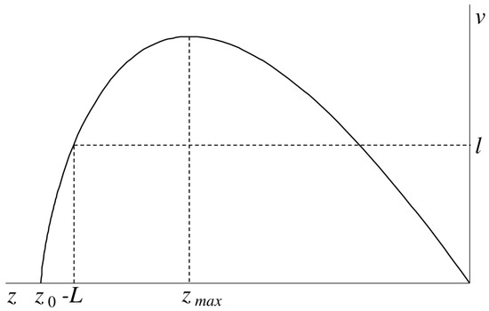
In other cases, the solution of problem (54), (55) is nonmonotonic, it has a maximum at some point $z_{max}<0$, and it becomes zero at some point $z_0<z_{max}$; moreover, $\underset{z\to z_0+0}{lim}{u}^{\prime }\left(z\right)=\infty$. This means that problem (54), (55) (accordingly, problem (29), (52)) can be solved on the interval $z\in [-L,0]$ only when $z_0\le -L$, and problem (3), (4) has a solution only on the finite time interval $t\in [0,T]$, where $T=a^{-1}(-z_0{\mu }^{1-\theta }/A)$. The infinitely increasing derivative, as well as the fact that the value of $z_0$ is a priori unknown, makes it impossible to construct a solution to problem (54), (55) on the interval $z\in [z_0,0]$ by simply applying the IRBFCM. The solution can be constructed in two stages. At stage I, problem (54), (55) is solved by means of the IRBFCM on the interval $z\in [-L,0]$, where L is selected so that $v(-L)>0,v^{\prime }\left(L\right)>0$, i.e., $z_0<-L<z_{max}$, see Figure 2. At stage II, we change the variables in problem (54), (55) by changing the roles of the independent variable and the required function,

$$z^{″}=\frac{1}{v}\left[\frac{1}{\sigma }{z}^{\prime }+(v^{\theta }+1){\left(z^{\prime }\right)}^2+\left(B{v}^{\beta }+Cv\right){\left(z^{\prime }\right)}^3\right],v\in [0,l],$$

(56)

$$z\left(l\right)=-L,z^{\prime }\left(l\right)=-\frac{1}{v^{\prime }(-L)},$$

(57)

where the values $l=v(-L)$ and $v^{\prime }(-L)$ were found in stage I. Problem (56), (57) can also be solved by the IRBFCM. The constructed solution $z\left(v\right)$ enables us to find the value of $z_0=z\left(0\right)$, and its continuous form makes it possible to complete the solution of problem (54), (55) on the interval $z\in [z_0,-L]$.

Figure 2. A nonmonotonic solution to problem (54), (55).

8. Examples and Numerical Analysis

Due to nonlinearity and especially singularity, it is impossible to analytically prove the convergence of the proposed numerical method. It is hardly possible to estimate the order of convergence as well. Therefore, taking into account the proven existence of solutions, we estimate the correctness of the numerical solutions by comparison with known exact solutions and by evaluation of the equation residuals in the substitution of the solutions.

8.1. Estimating the Accuracy of the Cauchy Problem Solution

Let us first discuss the case of the linear wave front motion equation $a\left(t\right)=\mu t$. It follows from Equations (37)–(39) that, when $\theta =\beta$ and $B<\sigma$, all the coefficients of series (36) are positive and that the solution of problem (54), (55) decreases monotonically on the ray $z\in (-\infty ,0]$, i.e., the values of v increase as we move away from the point $z=0$ on this ray. If $B>\sigma$, the solution is nonmonotonic, and it exists only on an interval $z\in [z_0,0]$. Finally, when $B=\sigma$, problem (54), (55) has the exact solution:

$$v=-Bz.$$

(58)

In the latter case, solving the problem by the IRBFCM leads to the exact solution (58) at any values of $\sigma ,B,\beta$ even in the first iteration. This indicates the correctness of the algorithm.

The accuracy of solving problem (54), (55) by the IRBFCM when the exact solution is unknown is estimated by means of the residual of Equation (53) on the interval $z\in [-L,0]$ in the substitution of the obtained solution. Table 1 shows the values of residuals for the constructed monotonic solutions at $\sigma =3$, $\theta =1$, $\beta =1$, and $\epsilon ={10}^{-10}$ for different values of the parameter B, the interval length L, and the number of collocation points m. Multiquadrics [23,29] are hereinafter used as RBFs: $f_i\left(x\right)=\sqrt{1+{ϵ}^2{(x-x_i)}^2}$. The value of the shape parameter $ϵ$ is taken from [43].

Table 1. Residuals of (53) for monotonic solutions.

B	L	Solution, $\mathit{m}/\mathit{N}$	Residual	n
1	1	IRBFCM, $m=26$	$4.7·{10}^{-9}$	21
1	1	IRBFCM, $m=51$	$1.1·{10}^{-9}$	22
1	1	IRBFCM, $m=101$	$2.2·{10}^{-10}$	21
1	2	IRBFCM, $m=101$	$2.3·{10}^{-8}$	21
1	2.5	IRBFCM, $m=101$	$7.9·{10}^{-8}$	20
1	1	MPS, $N=10$	$4.4·{10}^{-5}$	-
1	1	MPS, $N=20$	$2.1·{10}^{-9}$	-
1	1	MPS, $N=30$	$5.8·{10}^{-14}$	-
1	2	MPS, $N=30$	$7.9·{10}^{-5}$	-
1	2.5	MPS, $N=30$	$6.6·{10}^{-2}$	-
2	1	IRBFCM, $m=26$	$2.5·{10}^{-9}$	20
2	1	IRBFCM, $m=51$	$3.7·{10}^{-10}$	21
2	1	IRBFCM, $m=101$	$2.9·{10}^{-11}$	21
2	4	IRBFCM, $m=101$	$5.2·{10}^{-9}$	20
2	5	IRBFCM, $m=101$	$4.4·{10}^{-8}$	20
2	1	MPS, $N=10$	$3.8·{10}^{-7}$	-
2	1	MPS, $N=20$	$8.5·{10}^{-15}$	-
2	1	MPS, $N=30$	$5.1·{10}^{-19}$	-
2	4	MPS, $N=30$	$2.2·{10}^{-4}$	-
2	5	MPS, $N=30$	$1.0·{10}^{-2}$	-

Additionally, to estimate the rate of convergence, Table 1 shows the number of iterations n at which $\epsilon$ becomes less than ${10}^{-10}$. About twenty iterations are sufficient.

For comparison, Table 1 also shows the values of residuals for the corresponding solutions in the form of the truncated series:

$$v=\sum _{k=0}^N\frac{v_k}{k!}{z}^k,v_k=v^{\left(k\right)}\left(0\right),$$

(59)

whose coefficients in the case of positive integer values of $\beta$ and $\theta$ are determined by the following recurrent formulas:

$$v_0=0,v_1=-\sigma ,$$

$$v_{n+1}=\frac{1}{1+n\sigma }\left[\sum _{k=2}^n\left(C_n^k+\frac{C_n^{k-1}}{\sigma }\right)v_k{v}_{n-k+2}+\sum _{\genfrac{}{}{0pt}{}{i_1,\dots ,i_{\theta }=0,}{i_1+\dots +i_{\theta }=n}}^n{C}_n^{i_1,\dots ,i_{\theta }}{v}_{i_1+1}{v}_{i_2}\dots v_{i_{\theta }}+\right.$$

$$\left.B\sum _{\genfrac{}{}{0pt}{}{i_1,\dots ,i_{\beta }=0,}{i_1+\dots +i_{\beta }=n}}^n{C}_n^{i_1,\dots ,i_{\beta }}{v}_{i_1}{v}_{i_2}\dots v_{i_{\beta }}+C{v}_n\right],n=1,2,\dots$$

(60)

The relations expressed by (60) result from successive differentiation of Equation (55). Taking into account that $v_0=0$, we can easily demonstrate that the right-hand side of the expression for $v_{n+1}$ depends on the coefficients with numbers not exceeding n.

The analysis of the obtained results suggests the following inferences. The accuracy of the solution obtained by the method of power series (MPS) near the initial instant can be higher than that of the numerical solution, yet it strongly depends on the problem parameters. As we move away from the initial instant, the accuracy of the truncated series decreases considerably, and starting from a certain instant there is a divergence of the MPS. The accuracy of the IRBFCM solution increases with the increasing number of collocation points; this testifies to the convergence of the iterative algorithm. Herewith, the increase in the length of the interval for which a solution is constructed does not cause a considerable decrease in accuracy. Note that the values of the equation parameters do not noticeably affect accuracy. Another advantage of the IRBFCM is that, as distinct from the MPS, it can be used with noninteger values of $\theta$ and $\beta$. Thus, the proposed numerical method is fairly universal, and it provides acceptable accuracy. This gives grounds to use the obtained solutions of problem (54), (55) as reference ones for the verification of the stepwise algorithm proposed above for solving problem (3), (4).

In what follows, we analyze the accuracy of two nonmonotonic solutions shown in Figure 3, graphs 1 and 2. Table 2 shows the residuals of Equation (53) separately on the intervals of monotonicity $z\in [v_{max},0]$, where the numerical solution is constructed at the stage I, and on the entire domain of definition $z\in [v_0,0]$, where the numerical solution is joined from the results of both stages. The calculations show that the accuracy of the nonmonotonic solutions is lower than that of the monotonic ones, and this is natural. The IRBFCM solution accuracy in stage II is lower than in stage I, yet satisfactory. Besides, note again convergence with respect to the number of collocation points. Note that the rate of convergence is close to one in Table 1. The MPS solution has a sufficient accuracy only on the interval $z\in [v_{max},0]$. Evidently, the interval $z\in [v_{max},v_0]$ goes beyond the domain of convergence. Certainly, this causes the worst performance of the MPS. Nevertheless, the MPS solutions can be used to select L in stage I of the numerical solution.

Figure 3. The nonmonotonic solutions of problem (54), (55) at $\sigma =3$, $\theta =1$: (1) $\beta =1$, $B=4$, $C=0$; (2) $\beta =2$, $B=2$, $C=0$; (3) $\beta =2$, $B=1$, $C=5$; (4) $\beta =2$, $B=2$, $C=1$.

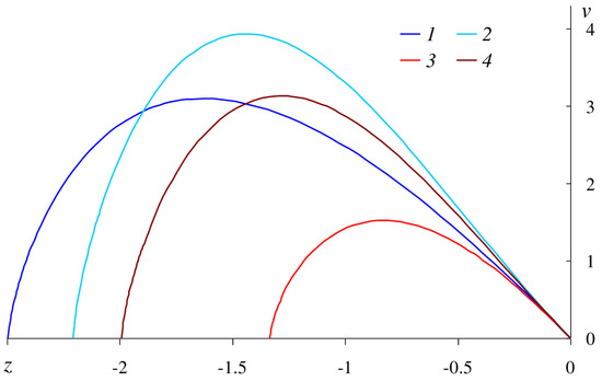
Table 2. Residuals of Equation (53) for nonmonotonic solutions at the linear function $a\left(t\right)$.

B	$\mathit{\beta }$	Solution, $\mathit{m}/\mathit{N}$	Residual in $[{\mathit{v}}_{max},0]$	Residual in $[{\mathit{v}}_0,0]$
4	1	IRBFCM, $m=26$	$5.4·{10}^{-5}$	$2.4·{10}^{-3}$
4	1	IRBFCM, $m=51$	$9.4·{10}^{-7}$	$6.1·{10}^{-4}$
4	1	IRBFCM, $m=101$	$5.7·{10}^{-8}$	$8.7·{10}^{-5}$
4	1	MPS, $N=10$	$1.8·{10}^{-1}$	$21.1$
4	1	MPS, $N=20$	$2.9·{10}^{-3}$	$41.3$
4	1	MPS, $N=30$	$4.6·{10}^{-5}$	$53.7$
2	2	IRBFCM, $m=26$	$3.9·{10}^{-4}$	$7.2·{10}^{-3}$
2	2	IRBFCM, $m=51$	$9.5·{10}^{-6}$	$5.1·{10}^{-4}$
2	2	IRBFCM, $m=101$	$1.9·{10}^{-7}$	$7.7·{10}^{-5}$
2	2	MPS, $N=10$	$3.7·{10}^{-1}$	$38.0$
2	2	MPS, $N=20$	$9.7·{10}^{-3}$	$63.4$
2	2	MPS, $N=30$	$3.4·{10}^{-4}$	$73.9$

Note that the inequality $\alpha >\gamma$ holds for solution 1, hence $p_1>0$ (see Equation (38)); consequently, $v^{″}\left(0\right)<0$, and solution 1 is convex in some vicinity of the point $z=0$. The calculations show that this property is preserved in the entire domain of definition. The inequality $\alpha <\gamma$ is valid for solution 2, hence $v^{″}\left(0\right)>0$, and there is an inflexion, which, as the calculations show, is reached at the point $z=-0.4651$. Note that in earlier studies of similar problems, which were performed by both numerical [44,45] and analytical [12,37] methods, these effects were not detected, although they had been expected.

When the function $a\left(t\right)$ has a logarithmic form, the solution of problem (54), (55) is always nonmonotonic. Table 3 shows the residuals of Equation (53) for the other two solutions presented in Figure 3, graphs 3 and 4. The results are similar to those obtained for the case of the linear function $a\left(t\right)$ and shown in Table 2. Note that $\sigma <C$ is valid for solution 3; this leads to the inequality $p_1>0$ and then to the convexity on the entire domain of definition. For solution 4, on the contrary, $\sigma >C$, $p_1<0$, and there is an inflection at the point $z=-0.3124$.

Table 3. Residuals of Equation (53) for nonmonotonic solutions at the logarithmic function $a\left(t\right)$.

B	C	Solution, $\mathit{m}/\mathit{N}$	Residual in $[{\mathit{v}}_{max},0]$	Residual in $[{\mathit{v}}_0,0]$
1	5	IRBFCM, $m=26$	$8.3·{10}^{-4}$	$5.7·{10}^{-3}$
1	5	IRBFCM, $m=51$	$2.9·{10}^{-5}$	$5.9·{10}^{-4}$
1	5	IRBFCM, $m=101$	$1.8·{10}^{-7}$	$9.2·{10}^{-5}$
1	5	MPS, $N=10$	$7.9·{10}^{-2}$	$17.9$
1	5	MPS, $N=20$	$7.8·{10}^{-4}$	$29.5$
1	5	MPS, $N=30$	$7.2·{10}^{-6}$	$37.6$
2	1	IRBFCM, $m=26$	$1.6·{10}^{-4}$	$2.7·{10}^{-3}$
2	1	IRBFCM, $m=51$	$8.2·{10}^{-6}$	$9.5·{10}^{-4}$
2	1	IRBFCM, $m=101$	$3.9·{10}^{-7}$	$1.7·{10}^{-4}$
2	1	MPS, $N=10$	$2.1·{10}^{-1}$	$29.8$
2	1	MPS, $N=20$	$3.2·{10}^{-3}$	$52.3$
2	1	MPS, $N=30$	$4.4·{10}^{-5}$	$67.4$

8.2. Estimating the Accuracy of the Stepwise Solution of Problem (3), (4)

To verify the algorithm of the numerical solution of problem (3), (4) discussed in Section 3, we use the reference solution corresponding to the constructed solution of problem (54), (55).

Note that, when problem (54), (55) has the exact solution (58), the IRBFCM at each step leads to the corresponding linear solution of problem (3), (4) in the first iteration.

To illustrate the work of the algorithm, we adduce the calculation results for $\sigma =3$, $\theta =1$, $\beta =1$, $A=1$, $B=1$, $a\left(t\right)=\mu t$, $\mu =0.5$ in problem (3), (4). The corresponding problem (54), (55) was solved for $\theta =1$, $\beta =1$, $B=2$, $L=1$, $m=101$, $\epsilon ={10}^{-10}$, the residual of Equation (53) was $2.9·{10}^{-11}$. At each time step, the highest deviation of the numerical solution from the reference one was reached at $x=0$, this being attributable to the form of the boundary condition (4). Therefore, the relative deviation of the stepwise solution from the reference one at $x=0$ is taken as the error estimate. Table 4 shows the values of this deviation at two time instants for different values of the time step h and the number of collocation points m. The calculations were made for two time difference schemes: first-order and second-order ones (Equations (18) and (22), respectively). The calculation results demonstrate a good accuracy of the IRBFCM, as well as convergence with respect to time step and the number of collocation points. The number of collocation points has a greater effect on the result than the step size. Note that the application of the second-order time difference scheme instead of the first-order one significantly increases the accuracy of the solution.

Table 4. Stepwise solution errors for $a\left(t\right)=0.5t$ at $x=0$.

t	h	m	Diff. Scheme Order	Error
0.5	0.1	51	1	0.010349
0.5	0.1	101	1	0.009864
0.5	0.1	201	1	0.009658
0.5	0.05	51	1	0.007123
0.5	0.05	101	1	0.006624
0.5	0.05	201	1	0.006414
0.5	0.02	51	1	0.004084
0.5	0.02	101	1	0.003568
0.5	0.02	201	1	0.003354
0.5	0.1	51	2	0.002101
0.5	0.1	101	2	0.001199
0.5	0.1	201	2	0.000753
0.5	0.05	51	2	0.001717
0.5	0.05	101	2	0.000902
0.5	0.05	201	2	0.000509
0.5	0.02	51	2	0.001376
0.5	0.02	101	2	0.000672
0.5	0.02	201	2	0.000339
1	0.1	51	1	0.015057
1	0.1	101	1	0.014008
1	0.1	201	1	0.013567
1	0.05	51	1	0.009884
1	0.05	101	1	0.008864
1	0.05	201	1	0.008412
1	0.02	51	1	0.005780
1	0.02	101	1	0.004656
1	0.02	201	1	0.004199
1	0.1	51	2	0.003857
1	0.1	101	2	0.002151
1	0.1	201	2	0.001325
1	0.05	51	2	0.003057
1	0.05	101	2	0.001603
1	0.05	201	2	0.000886
1	0.02	51	2	0.002583
1	0.02	101	2	0.001218
1	0.02	201	2	0.000599

Similar calculations were made for the case when the function $a\left(t\right)$ is logarithmic. Problem (3), (4) was solved with $\sigma =3$, $\theta =1$, $\beta =2$, $A=1$, $B=2$, $a\left(t\right)=\omega ln(\mu t+\eta )$, $\omega =1$, $\mu =1$, and $\eta =1$. The corresponding problem (54), (55) was solved with $\theta =1$, $\beta =2$, $B=2$, $C=5$, $L=0.7$, $m=101$, and $\epsilon ={10}^{-10}$, the residual of Equation (53) being $2.8·{10}^{-10}$. The results shown in Table 5 demonstrate convergence with respect to time step both for the first-order and second-order time difference schemes. For the first-order scheme, there is no convergence with respect to the number of collocation points; the errors are greater than those for the linear function $a\left(t\right)$. On the contrary, when the second-order scheme is used, convergence with respect to the number of collocation points is observed, and the errors are close to those for the linear function $a\left(t\right)$. Obviously these results are explainable by the nonlinearity of $a\left(t\right)$, and they demonstrate the advantage of the new second-order time difference scheme.

Table 5. Stepwise solution errors for $a\left(t\right)=\ln (t+1)t$ at $x=0$.

t	h	m	Diff. Scheme Order	Error
0.5	0.1	51	1	0.033855
0.5	0.1	101	1	0.034556
0.5	0.1	201	1	0.034844
0.5	0.05	51	1	0.020623
0.5	0.05	101	1	0.021296
0.5	0.05	201	1	0.021589
0.5	0.02	51	1	0.009334
0.5	0.02	101	1	0.010126
0.5	0.02	201	1	0.010338
0.5	0.1	51	2	0.004718
0.5	0.1	101	2	0.003992
0.5	0.1	201	2	0.003628
0.5	0.05	51	2	0.002347
0.5	0.05	101	2	0.001713
0.5	0.05	201	2	0.001405
0.5	0.02	51	2	0.001252
0.5	0.02	101	2	0.000711
0.5	0.02	201	2	0.000430
1	0.1	51	1	0.033389
1	0.1	101	1	0.034664
1	0.1	201	1	0.035185
1	0.05	51	1	0.017711
1	0.05	101	1	0.019214
1	0.05	201	1	0.019852
1	0.02	51	1	0.006753
1	0.02	101	1	0.008277
1	0.02	201	1	0.008540
1	0.1	51	2	0.005023
1	0.1	101	2	0.003948
1	0.1	201	2	0.003419
1	0.05	51	2	0.002541
1	0.05	101	2	0.001661
1	0.05	201	2	0.001222
1	0.02	51	2	0.001734
1	0.02	101	2	0.000631
1	0.02	201	2	0.000625

9. Conclusions

This paper has studied the construction of diffusion wave type solutions, whose existence was proved earlier in [10], for a second-order quasilinear parabolic equation with a singularity. A stepwise algorithm based on an RBF collocation method has been proposed for a numerical solution of the equation with a specified law of diffusion front motion. The first- and second-order difference schemes have been constructed for time discretization. At each time step, the problem is solved iteratively, with the application of the particular solution method and the RBF collocation method. To verify the developed numerical method, two classes of exact solutions of the generalized traveling wave type have been proposed, whose construction is reduced to solving a Cauchy problem for ODE with a singularity at the higher derivative. For this problem, the theorem of the existence and uniqueness of the local analytical solution in the form of a power series has been proved. The properties of this series have been studied and convergence radius estimates have been made, which enable constructive conditions for the applicability of truncated series to be obtained for calculations. The Euler method is used to prove the existence of a solution to the Cauchy problem in the case when the equation has finite smoothness and there is no analytical solution. The case when the Cauchy problem has an exact solution in the finite form has been selected. The iteration RBF collocation method has been proposed for solving the Cauchy problem numerically. The computing experiment and the numerical analysis have resulted in the following conclusions:

1.

In some cases the solution of the Cauchy problem is monotonic on an infinite interval, and this allows one to construct a solution to the original problem for an arbitrary time instant;

2.

In other cases, the solution to the Cauchy problem is nonmonotonic; it is defined on a finite interval and has a maximum inside this interval. This means that the solution of the original problem is restricted and that it exists on a finite time interval;

3.

For restricted solutions defined on a finite time interval, a point at which the second derivative changes its sign (inflection point) can appear. These effects failed to be revealed earlier in studying similar problems, although, according to general reasoning, they were supposed to exist;

4.

The accuracy of solving the Cauchy problem by the IRBFCM is fairly high, and this enables the thus constructed solutions of the original problem to be used to verify the developed stepwise algorithm;

5.

The verification of the stepwise algorithm indicates the convergence of the IRBFCM in each step, good solution accuracy, and a considerable advantage of the second-order time difference scheme. Further studies along this line can deal, first of all, with the further development of the algorithmic tool and its extension to the problem with given boundary conditions generating a diffusion wave. This problem is more complicated but more interesting for applications. Besides, a very ambitious challenge is to prove rigorous mathematical statements about the convergence of the developed algorithm. However, the general solvability of this problem is questionable, and it can most likely be solved only in particular cases.

In conclusion, note that the extension of the results to the cases of two and three spatial variables is an important problem to be solved. This step is necessary since we participate in the development of a modeling-algorithmic approach to solving problems of the evolution of the ice cover and biota of lake Baikal (included in the UNESCO World Heritage List), and this implies solving nonlinear parabolic equations and systems.

References

- Vazquez, J. The Porous Medium Equation: Mathematical Theory; Clarendon Press: Oxford, UK, 2007. [Google Scholar] [CrossRef]
- Samarskii, A.; Galaktionov, V.; Kurdyumov, S.; Mikhailov, A. Blow-Up in Quasilinear Parabolic Equations; Walter de Gruyte: Berlin, Germany, 1995. [Google Scholar] [CrossRef]
- Evans, L. Partial Differential Equations; American Mathematical Society: Providence, RI, USA, 2010. [Google Scholar] [CrossRef] [Green Version]
- Barenblatt, G.; Entov, V.; Ryzhik, V. Theory of Fluid Flows Through Natural Rocks; Kluwer Academic Publishers: Dordrecht, The Netherlands, 1990. [Google Scholar]
- Zeldovich, Y.B.; Raizer, Y.P. Physics of Shock Waves and High-Temperature Hydrodynamic Phenomena; Dover Publications: New York, NY, USA, 2002. [Google Scholar] [CrossRef]
- Murray, J. Mathematical Biology: I. An Introduction, 3rd ed.; Interdisciplinary Applied Mathematics; Springer: New York, NY, USA, 2002; Volume 17. [Google Scholar] [CrossRef]
- Achouri, T.; Ayadi, M.; Habbal, A.; Yahyaoui, B. Numerical analysis for the two-dimensional Fisher-Kolmogorov-Petrovski-Piskunov equation with mixed boundary condition. J. Appl. Math. Comput. 2021. [CrossRef]
- Ershkov, S.V.; Leshchenko, D. Note on semi-analytical nonstationary solution for the rivulet flows of non-Newtonian fluids. Math. Meth. Appl. Sci. 2022, 1–10. [Google Scholar] [CrossRef]
- Kazakov, A.L. On exact solutions to a heat wave propagation boundary-value problem for a nonlinear heat equation. Sib. Electron. Math. Rep. 2019, 16, 1057–1068. [Google Scholar] [CrossRef]
- Kazakov, A. Solutions to Nonlinear Evolutionary Parabolic Equations of the Diffusion Wave Type. Symmetry 2021, 13, 871. [Google Scholar] [CrossRef]
- Kazakov, A.L.; Kuznetsov, P.A. On the Analytic Solutions of a Special Boundary Value Problem for a Nonlinear Heat Equation in Polar Coordinates. J. Appl. Ind. Math. 2018, 812, 227–235. [Google Scholar] [CrossRef]
- Kazakov, A.; Lempert, A. Diffusion-Wave Type Solutions to the Second-Order Evolutionary Equation with Power Nonlinearities. Mathematics 2022, 10, 232. [Google Scholar] [CrossRef]
- Kazakov, A.; Spevak, L. An analytical and numerical study of a nonlinear parabolic equation with degeneration for the cases of circular and spherical symmetry. Appl. Math. Model. 2016, 40, 1333–1343. [Google Scholar] [CrossRef]
- Kazakov, A.L.; Nefedova, O.A.; Spevak, L.F. Solution of the Problem of Initiating the Heat Wave for a Nonlinear Heat Conduction Equation Using the Boundary Element Method. Comput. Math. Math. Phys. 2019, 59, 1015–1029. [Google Scholar] [CrossRef]
- Kazakov, A.; Spevak, L.; Nefedova, O.; Lempert, A. On the Analytical and Numerical Study of a Two-Dimensional Nonlinear Heat Equation with a Source Term. Symmetry 2020, 12, 921. [Google Scholar] [CrossRef]
- Brebbia, C.A.; Telles, J.C.F.; Wrobel, L.C. Boundary Element Techniques; Springer: Berlin/Heidelberg, Germany, 1984. [Google Scholar] [CrossRef]
- Nardini, D.; Brebbia, C. A new approach to free vibration analysis using boundary elements. Appl. Math. Model. 1983, 7, 157–162. [Google Scholar] [CrossRef]
- Wrobel, L.; Brebbia, C. The Dual Reciprocity Boundary Element Formulation for Nonlinear Diffusion Problems. Comput. Methods Appl. Mech. Eng. 1987, 65, 147–164. [Google Scholar] [CrossRef]
- Tanaka, M.; Matsumoto, T.; Takakuwa, S. Dual reciprocity BEM for time-stepping approach to the transient heat conduction problem in nonlinear materials. Comput. Methods Appl. Mech. Eng. 2006, 195, 4953–4961. [Google Scholar] [CrossRef]
- Divo, E.; Kassab, A.J. Transient Non-linear Heat Conduction Solution by a Dual ReciprocityBoundary Element Method with an Effective Posteriori Error Estimator. Comput. Mater. Contin. 2005, 2, 277–288. [Google Scholar] [CrossRef]
- Golberg, M.A.; Chen, C.S.; Bowman, H. Some recent results and proposals for the use of radial basis functions in the BEM. Eng. Anal. Bound. Elem. 1999, 23, 285–296. [Google Scholar] [CrossRef]
- Buhmann, M.D. Radial Basis Functions; Cambridge University Press: Cambridge, UK, 2003. [Google Scholar] [CrossRef]
- Kansa, E.J. Multiquadrics—A scattered data approximation scheme with applications to computational fluid-dynamics—II solutions to parabolic, hyperbolic and elliptic partial differential equations. Comput. Math. Appl. 1990, 19, 147–161. [Google Scholar] [CrossRef] [Green Version]
- Fedoseyev, A.I.; Friedman, M.J.; Kansa, E.J. Improved multiquadric method for elliptic partial differential equations via PDE collocation on the boundary. Comput. Math. Appl. 2002, 43, 439–455. [Google Scholar] [CrossRef] [Green Version]
- Chen, C.S.; Fan, C.M.; Wen, P.H. The method of approximate particular solutions for solving certain partial differential equations. Numer. Methods Partial. Differ. Equ. 2010, 28, 506–522. [Google Scholar] [CrossRef]
- Dou, F.; Liu, Y.; Chen, C.S. The method of particular solutions for solving nonlinear Poisson problems. Comput. Math. Appl. 2019, 77, 501–513. [Google Scholar] [CrossRef]
- Golberg, M.A. The method of fundamental solutions for Poisson’s equation. Eng. Anal. Bound. Elem. 1995, 16, 205–213. [Google Scholar] [CrossRef]
- Fairweather, G.; Karageorghis, A. The method of fundamental solution for elliptic boundary value problems. Adv. Comput. Math. 1998, 9, 69–95. [Google Scholar] [CrossRef]
- Chen, C.S.; Chen, W.; Fu, Z.J. Recent Advances in Radial Basis Function Collocation Methods; Springer: Berlin/Heidelberg, Germany, 2013. [Google Scholar]
- Fornberg, B.; Flyer, N. Solving PDEs with radial basis functions. Acta Numer. 2015, 24, 215–258. [Google Scholar] [CrossRef] [Green Version]
- Myers, D.; Iaco, S.D.; Posa, D.; Cesare, L.D. Space-time radial basis functions. Comput. Math. Appl. 2002, 43, 539–549. [Google Scholar] [CrossRef] [Green Version]
- Zerroukat, M.; Power, H.; Chen, C.S. A numerical method for heat transfer problems using collocation and radial basis functions. Int. J. Numer. Methods Eng. 1998, 42, 1263–1278. [Google Scholar] [CrossRef]
- Li, J.; Hon, Y.; Chen, C. Numerical comparisons of two meshless methods using radial basis functions. Eng. Anal. Bound. Elem. 2002, 26, 205–225. [Google Scholar] [CrossRef]
- Leontiev, N.E.; Roshchin, E.I. Exact Solutions to the Deep Bed Filtration Problem for Low-Concentration Suspension. Mosc. Univ. Mech. Bull. 2020, 75, 96–101. [Google Scholar] [CrossRef]
- Polyanin, A.D.; Zaitsev, V.F. Handbook of Nonlinear Partial Differential Equations, 2nd ed.; Chapman and Hall/CRC: New York, NY, USA, 2012. [Google Scholar] [CrossRef]
- Sinelshchikov, D.I. Nonlocal deformations of autonomous invariant curves for Liénard equations with quadratic damping. Chaos Solitons Fractals 2021, 152, 111412. [Google Scholar] [CrossRef]
- Kazakov, A.L.; Orlov, S.S.; Orlov, S.S. Construction and study of exact solutions to a nonlinear heat equation. Sib. Math. J. 2018, 59, 427–441. [Google Scholar] [CrossRef]
- Filimonov, M.Y.; Vaganova, N.A. Application of series with recurrently calculated coefficients for solving initial-boundary value problems for nonlinear wave equations. In Proceedings of the Thermophysical Basis of Energy Technologies (TBET 2020), Tomsk, Russia, 28–30 October 2020; AIP Publishing: College Park, MD, USA, 2021. [Google Scholar] [CrossRef]
- Filimonov, M.Y.; Korzunin, L.G.; Sidorov, A.F. Approximate Methods for Solving Nonlinear Initial Boundary-Value Problems Based on Special Constructions of Series. Russ. J. Numer. Anal. Math. Model. 1993, 8, 101–126. [Google Scholar] [CrossRef]
- Kazakov, A.; Spevak, L. Numerical and analytical studies of a nonlinear parabolic equation with boundary conditions of a special form. Appl. Math. Model. 2013, 37, 6918–6928. [Google Scholar] [CrossRef]
- Hayek, M. A family of analytical solutions of a nonlinear diffusion–convection equation. Phys. A Stat. Mech. Appl. 2018, 490, 1434–1445. [Google Scholar] [CrossRef]
- Pudasaini, S.P.; Hajra, S.G.; Kandel, S.; Khattri, K.B. Analytical solutions to a nonlinear diffusion–advection equation. Z. Angew. Math. Phys. 2018, 69, 150. [Google Scholar] [CrossRef]
- Franke, R. Scattered data interpolation: Tests of some methods. Math. Comput. 1982, 38, 181–200. [Google Scholar] [CrossRef]
- Kazakov, A.L.; Spevak, L.F.; Lee, M.G. On the Construction of Solutions to a Problem with a Free Boundary for the Non-linear Heat Equation. J. Sib. Fed. Univ. Math. Phys. 2020, 13, 694–707. [Google Scholar] [CrossRef]
- Kazakov, A.L.; Spevak, L.F. Approximate and Exact Solutions to the Singular Nonlinear Heat Equation with a Common Type of Nonlinearity. Bull. Irkutsk. State Univ. Ser. Math. 2020, 34, 18–34. [Google Scholar] [CrossRef]
Publisher’s Note: MDPI stays neutral with regard to jurisdictional claims in published maps and institutional affiliations. |
© 2022 by the authors. Licensee MDPI, Basel, Switzerland. This article is an open access article distributed under the terms and conditions of the Creative Commons Attribution (CC BY) license (https://creativecommons.org/licenses/by/4.0/).