Deep Learning XAI for Bus Passenger Forecasting: A Use Case in Spain

Abstract

Time series forecasting of passenger demand is crucial for optimal planning of limited resources. For smart cities, passenger transport in urban areas is an increasingly important problem, because the construction of infrastructure is not the solution and the use of public transport should be encouraged. One of the most sophisticated techniques for time series forecasting is Long Short Term Memory (LSTM) neural networks. These deep learning models are very powerful for time series forecasting but are not interpretable by humans (black-box models). Our goal was to develop a predictive and linguistically interpretable model, useful for decision making using large volumes of data from different sources. Our case study was one of the most demanded bus lines of Madrid. We obtained an interpretable model from the LSTM neural network using a surrogate model and the 2-tuple fuzzy linguistic model, which improves the linguistic interpretability of the generated Explainable Artificial Intelligent (XAI) model without losing precision.

1. Introduction

Efficient passenger transport in urban areas is an increasingly important problem in our society. In the past few years, it was empirically shown that constructing new infrastructures or expanding existing roads is not an adequate solution to this problem. However, the use of public transport should be encouraged to try to alleviate effects such as congestion, accidents and pollution [1].

Knowledge of passenger demand is crucial for decisions related to planning the supply of public transport services, as well as for the design of lines based on demand. Passenger demand depends on many factors: population, income, commercial and service establishments, while other factors depend solely on the transport offer, such as travel time, frequencies offered and comfort. To achieve maximum efficiency in the service, it is essential to know the passenger demand over time, since it is usually characterized by high seasonality with annual, weekly or daily peak periods.

Most public transport systems have frequent delays due to poor planning of the different routes, leading to crowded transport on certain routes and completely empty on others. This mismanagement of public transport also has other consequences, which have an impact not only on the lives of its users, but also on the people who do not travel on them.

This paper focuses on the bus passenger demand problem. In this way, poor planning of bus routes can cause congestion on the streets, which can make it difficult for those using private vehicles to get around. It can cause overcrowding at bus stops if not enough buses are assigned to the busiest routes. Preventing these and other public transport problems requires good passenger demand planning.

In this sense, there is currently a large amount of data due to the fact that we live in a totally connected world. For good planning of bus passenger demand, it is necessary to have a detailed description and analysis of travel information that will allow us to adopt the most appropriate technical or political measures. Therefore, it is necessary to obtain accurate and reliable information about trips, such as frequency, duration, type of transport and costs. Through the Internet of Things (IoT), all the data can be collected throughout the entire journey, from the passenger pick-up, the time and the stop. This real-time data collection, as well as its subsequent analysis and study, will provide all the information necessary to implement and optimize the processes involved in demand planning, in addition to helping strategic and efficient decision-making [2].

Time series forecasting of bus passenger demand is crucial for an optimal planning of the limited resources. This is usually a complex task where nonlinear statistical relations between predictors and target variable must be identified. Long-short-term memory networks (LSTM) are a type of recurrent neural network used in deep learning [3,4] that can be trained to successfully handle sequence dependency. In fact, LSTMs are often used to predict passenger demand.

A problem with these “black box” models is that it is difficult to explain in detail the internal operations beyond the function provided by each of the layers and the symmetries of the model. However, interpretability of the model is crucial for transparency, traceability, and auditability, especially in public resources allocation. Therefore, the interpretation of such algorithms using XAI techniques is crucial.

Our goal is to develop a predictive and linguistically interpretable model, useful for decision making using large volumes of data, and able to work with various sources including the calendar, that predicts bus passenger demand. Our case will be one of the most demanded bus lines of Madrid.

The original data source has been provided by Empresa Municipal de Transportes de Madrid, EMT (Municipal Transport Company of Madrid, Spain) via email request. It includes the passenger data history of its entire fleet of buses, including night buses from 1 January 2015 to 28 February 2017. These data were obtained from the bus machines that registered the entry of passengers. Every time a passenger inserts their ticket or subscription in the machine, it generates a new entry in the database and is registered as a new trip.

To achieve the goal, we have relied on the explainability of the algorithm developed using deep learning techniques [3,4]. In our project we will focus only on LSTM neural networks [5,6], used for the prediction of time series, since a comparison of models was made and this algorithm was the most predictive.

For this, we first proposed to improve the prediction of passenger demand through historical data and external sources, such as calendar, through the use of deep learning techniques using deep neural LSTM networks. The goal is to make urban transport more efficient, ensuring that the offer meets the requirements of the population. However, LSTM models are “black boxes” which are very difficult to interpret. In many practical cases, this prevents the application of the model as the decisions of the model cannot be audited [7].

Surrogate models, however, can be highly interpretable from a business point of view. However, in the case we are dealing with in this paper, we have a large volume of data on a large number of means of transport, each of which will be explained by a different surrogate model. In this case, interpretability is reduced as the regression trees usually have several end nodes with precise values of the dependent variable that must be interpreted relative to each specific means of transport. Thus, 2000 passengers may be an extreme figure for a particular bus line or a low number for another. To increase the interpretability of these variables, we propose the use of fuzzy linguistic variables which were originally proposed by Zadeh [8]. This type of variable is based on fuzzy sets that represent linguistic concepts normally handled by human beings, for example, with reference to a means of transport, it is easy to interpret that the number of passengers is high or medium. In order to increase interpretability, we propose the use of the fuzzy 2-tuple linguistic model. The advantage of this model is that it allows such interpretability in addition to achieving greater precision in the representation and computation of these fuzzy concepts.

The rest of article is structured as follows: Section 2 presents the state of the art and compares these related works to our proposal; Section 3 presents foundations of deep learning, fuzzy models and XAI on which our proposal is based; Section 4 presents the model for bus passenger demand forecasting and obtaining its interpretation, the model is applied to data from the city of Madrid (Spain); in Section 5, the results obtained by this model are discussed; and finally, in Section 6, conclusions and future work are suggested.

2. Related Works

The problem raised in this paper can be considered within the field of smart public transport. This is one of the most important issues for so-called smart cities [9]. Intelligent transport focuses on controlling and managing transport networks and systems to improve safety and efficiency. In such problems, there are multitudes of devices generating huge amounts of data. Based on such data, a crucial issue for decision making in a smart city is the prediction related to traffic flow [10], travel times [11], congestion prevention, or passenger demand, among others.

Our proposal focuses on forecasting of public bus passenger demand through deep learning techniques, and in this section, we will first study the background of this type of work in the literature. For this purpose, we will conduct a bibliometric study on this topic. Specifically, we will draw a bibliometric map. This type of map is part of the science mapping, which aims to obtain a conceptual structure of a given area prior to its interpretation. We follow the methodology based on [12] and the SciMat tool in order to obtain such map.

In the first stage, the data, i.e., the articles that compose the analysis, must be retrieved. Thus, bibliographic records were downloaded from the main Web of Science collection using the query: TS = ((“forecast*” OR “prediction*”) NEAR/6 (“passenger” or “traveler” or “traveller” or “voyager”) AND (“machine learning” or “deep learning”)) where the TS field is a search based on a given topic (title, abstract and keywords), NEAR/n is a proximity operator that requires both terms to appear close to each other, up to n-words, in the text. The query was run at the end of March 2022 and returned 120 documents which were manually reviewed.

In the next phase, pre-processing, we unify term duplicates and fixed misspelled items.

Thereafter, we carry out the remaining phases of the process: network extraction, normalization, mapping, analysis and visualization.

An advantage of the methodology followed is that it allows us to obtain a strategic diagram of the topics based on two measures: centrality, i.e., degree of interaction of a network with other networks and density, i.e., the internal strength of the network or keywords that describe the theme in any science mapping workflow. We show the strategic diagram obtained for our analysis in Figure 1 including the interpretation of the topics of each quadrant.

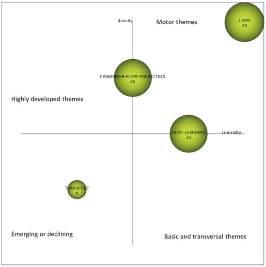
Figure 1. Strategic map of prediction of passegers using machine/deep learning in the literature.

We can identify four main themes, on which Figure 2 shows their thematic networks:

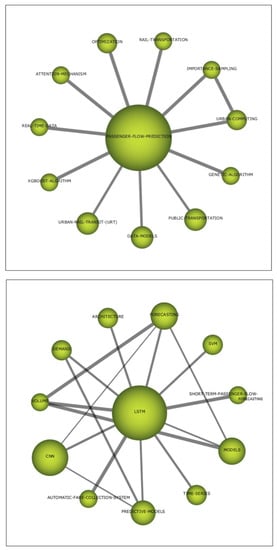
Figure 2. Thematic networks for each theme.

• DEEP-LEARNING. Based on neural networks, this algorithms are widely used for the traffic flow prediction problem presented here.
• LSTM. This theme includes specific deep/machine learning algorithms which are important or motor for the problem at hand. Thus, LSTM models are the central and predominant topic, the Convolutional Neural Networks (CNN) are in second place, and finally, Support Vector Machine (SVM) is much less prominent. The theme is related with time model prediction since in the problems we are dealing with, they are very common.
• PASSENGER-FLOW-PREDICTION. This is a heterogeneous topic that includes the optimization problems and techniques studied, including genetic algorithms. It also includes other predictive techniques such as XGBoost. This theme includes other interesting terms that point to the use of real-time data and predictive applications on urban and public transportation.
• TRANSPORT. This is a very small and declining theme which includes the use of statistical analysis and generic machine learning for the problem posed.

Therefore, we consider in this work a model widely used in the related literature, the LSTM. On the other hand, the prediction of passengers involves various means of transport. Table 1 shows the work specifically related to buses. Our proposal is also included in this table.

Table 1. Bus passenger flow prediction related work.

Ref.	Fundamentals	Datasets	Application	Interpretation of Model
Lv et al., 2022 [13]	XGBoost	Passenger data and Point of Interest	Bus passenger flow prediction in Beijing (China)
Jin et al., 2018 [14]	Shepard model	Passenger data and multi-source data	Bus passenger flow Prediction
Jiao et al., 2021 [7]	STL (Locally Weighted Regression) and LSTM (Long Short-Term memory) based model	Passenger data, weather data, holiday data, etc.	Bus passenger flow prediction in Beijing (China)
Ouyang et al., 2020 [15]	Feature extraction based on XGBoost model and prediction based on LSTM	Historical and real-time passenger data and Point of Interest	Bus passenger flow prediction in Beijing (China)
Gummadi and Edara, 2019 [16]	Artificial Neural Network	Passenger flow data	Bus passenger flow prediction
Nagaraj et al., 2022 [17]	LSTM	Passenger flow data	Bus passenger flow prediction in in Karnataka State Road Transport Corporation Bus Rapid Transit (KSRTCBRT) transportation in India
Zhai et al., 2020 [18]	Hybrid model based on time series model (ARIMA), Deep Belief Networks (DBNs), and improved Incremental Extreme Learning Machine (Im-ELM)	Passenger flow data collected by the automatic passenger counting	Bus passenger flow prediction in Dalian (China)
Zou et al., 2022 [19]	XGBoost	Travel Card Data passenger data	Bus Passenger flow prediction in Guangzhou (China)	Contributions of variables to the prediction of passenger flow
Liu and Chen, 2017 [20]	Stacked Autoen- Coders (SAE) & Deep Neural Network (DNN)	Passenger flow data collected by the automatic passenger counting and holidays data	Bus rapid transit passenger flow prediction in Xiamen (China)
Chen et al., 2022 [21]	Spatial–Temporal Graph Sequence with Attention Network (STGSAN)	Passenger flow data	Bus passenger flow prediction in Urumqi (China)
Wu et al., 2020 [22]	Stacking Gradient Boosting Decision Tree (SS-GBDT)	Passenger flow data and multi-source information	Bus passenger flow prediction in Guangzhou (China)
Liu et al., 2020 [23]	Deep Neural Network and Modular Convolutional Neural Network	Passenger flow data	Bus & passenger flow prediction in Nanjing (China)
Liu et al., 2020b [24]	Support Vector Machine (SVM)	Passenger flow from bus station data and smart travel card data	Bus passenger flow prediction in Shenzhen Tong (China)
Tan et al., 2019 [25]	Random Forest	Smart travel card data	Bus passenger flow prediction in Shenzhen (China)
Bai et al., 2017 [26]	Multi-Pattern Deep Fusion (MPDF) based on Deep Belief Network	Passenger flow data	Bus passenger flow prediction in Guangzhou (China)
Han et al., 2019 [27]	LSTM	Passenger flow data	Bus passenger flow prediction in Qingdao (China)
Zhang et al., 2016 [28]	XGBoost	Passenger flow data, Point of Interests data and wheather data	Bus passenger boarding choices and public transit passenger flow in Guangzhou (China)
Luo et al., 2020 [29]	Multitask Deep-Learning (MDL) incluiding LSTM, CNN, etc.	Spatio-temporal and heterogenous flow data	Bus passenger flow prediction in Jinan (China)
Wang et al., 2022 [30]	LSTM and CNN	Spatio-temporal flow data	Bus passenger flow prediction
Toqué et al., 2017 [31]	LSTM, Random Forest, Neural Network	Bus passenger ticketing logs	Bus passenger flow prediction in Paris (France)
Zhai et al., 2018 [32]	Several Machine Learning methods: SVM, Neural Networks, ARIMA, etc.	Passenger flow data from automatic passenger counters, automatic fare collection systems…	Bus passenger flow prediction in Shanghai (China)
Our proposal	LSTM	Passenger flow data and holidays data	Bus passenger flow prediction in Madrid (Spain)	XAI Global Surrogate Model and 2-tuple Fuzzy Linguistic Model

As can be deduced from a review of the related literature, most of the machine learning algorithms used are so-called black box algorithms, i.e., they are able to predict but are not interpretable by humans. If we focus the analysis on bus passenger flow predictions, there are many works on this type of prediction, but very few authors have been concerned with the interpretability of the models, as can be seen in Table 1. The only works we found are limited to obtaining the importance of the variables involved in the model [19].

Therefore, interpreting the results of such algorithms using XAI techniques is appropriate, although on the other hand, they are still rather new techniques whose main field of action is still very generic and not so much focused on concrete problems [33,34]. Certainly, some work is oriented towards the field of smart cities [35,36,37,38] but specifically focused on public transport there are very few jobs. In this way, we can find works oriented to the prediction and understanding of traffic flow [39] and work [40], which seeks to make the recommendations on the transport fleet interpretable. To the best of our knowledge, there is no work specifically oriented to the problem of predictability and interpretability about public bus users as the work presented here.

There are several approaches that incorporate fuzzy logic-based techniques into the XAI problem [41], as will be shown in Section 3.3. The present work incorporates a fuzzy technique, called 2-tuple model that improves the linguistic interpretability of the generated XAI model without losing accuracy. We did not find in the literature the joint use of both approaches.

3. Methodology

The proposed model is based on three important models that will be explained in this section: the 2-tuple fuzzy linguistic model, the LSTM and surrogate trees and rules.

3.1. The 2-Tuple Fuzzy Linguistic Model

The 2-tuple model, proposed in [42], is a model that allows a more accurate representation of fuzzy linguistic terms of a linguistic variable without losing linguistic interpretability. For this reason, it is a model widely used in a variety of areas, i.e., [43,44]. This model represents the information as a pair of values ($s_i,{\alpha }_i$), where $s_i\in S$ and ${\alpha }_i\in \left[-0.5,0.5\right)$.

Definition 1

([42]). Let $S=s_0,\dots ,s_g$ be a set of linguistic terms, and $\beta \in \left[0,g\right]$ a value in the granularity interval of S. The symbolic translation of a linguistic term is a number valued in the interval [−0.5, 0.5) which expresses the difference in information between a given value $\beta \in \left[0,g\right]$ obtained from a symbolic operation, and the index of the closest linguistic term $s_i$ in S.

This representation model defines a pair of functions to perform transformations between numerical values defined in the granularity interval and 2-tuple linguistic values to perform the computational processes on 2-tuple linguistic values.

Definition 2

([42]). Let $S=s_0,\dots ,s_g$ be a set of linguistic terms, $⟨S⟩=S\times \left[-0.5,0.5\right)$ and $\beta \in \left[0,g\right]$ a value representing the result of a symbolic operation. Then the linguistic 2-tuple expressing information equivalent to $\beta$ is obtained using the following function:

$$\begin{gathered} {\Delta }_S:\left[0,g\right]\to ⟨S⟩ \\ {\Delta }_S\left(\beta \right)=\left(s_i,{\alpha }_i\right), \mathrm{with}\{i=round\left(\beta \right) \alpha =\beta -i, \alpha \in \left[-0.5,0.5\right), \end{gathered}$$

(1)

where $round\left(·\right)$ is the visual rounding operator, $s_i$ is the label with index closest to $\beta$ and $\alpha$ is the value of the symbolic translation.

Thus, a value in the interval $\left[0,g\right]$ is always identified with a 2-tuple linguistic value in $⟨S⟩$.

Definition 3.

Let$S=s_0,\dots ,s_g$be a set of linguistic terms and$\left(s_i,{\alpha }_i\right)\in ⟨S⟩=S\times \left[-0.5,0.5\right)$the numerical value in the granularity interval$\left[0,g\right]$representing the linguistic value 2-tuple$\left(s_i,{\alpha }_i\right)$is obtained using the function:

$$\begin{gathered} {\Delta }_S^{-1}: ⟨S⟩\to \left[0,g\right] \\ {\Delta }_S^{-1}\left(s_i,{\alpha }_i\right)=i+\alpha =\beta \end{gathered}$$

(2)

Along with the representation model seen above, we can analyse the associated computational model, for which the following operators are defined:

2-tuple linguistic value comparison operator. Given two 2-tuple linguistic values $\left(s_k,{\alpha }_1\right)$ and $\left(s_l,{\alpha }_2\right)$ representing quantities of information:

• If $k<l$, then $\left(s_k,{\alpha }_1\right)$ is less than $\left(s_l,{\alpha }_2\right)$.
• If $k=l$, then

  (a)

  If ${\alpha }_1={\alpha }_2$, then $\left(s_k,{\alpha }_1\right)$ and $\left(s_l,{\alpha }_2\right)$ represent the same information.

  (b)

  If ${\alpha }_1<{\alpha }_2$, then $\left(s_k,{\alpha }_1\right)$ is less than $\left(s_l,{\alpha }_2\right)$.

  (c)

  If ${\alpha }_1>{\alpha }_2$, then $\left(s_k,{\alpha }_1\right)$ is greater than $\left(s_l,{\alpha }_2\right)$.

The dependent variable, i.e., what we have to predict in this article is the number of passengers. As will be seen in Section 4, in order to improve the linguistic interpretability of this variable in the Machine Learning (ML) models obtained, we will represent this variable with this 2-tuple model. For this purpose, we define $S=\left\{s_0,\dots ,s_T\right\}$ with $T=4: s_o=Very Low=VL, s_1=Low=L, s_2=Medium=M, s_3=High=H, s_4=Very High=VH$, with the definition shown in Figure 3. Thus, for example, if in a given context, a model predicts a number of passengers (High, −0.1), we can interpret it as being well above Medium and well below Very High, and it is also below the High concept, namely 0.1 of semantic translation.

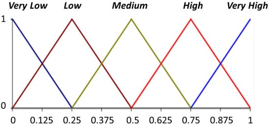
Figure 3. Definition of the set S for the variable “number of passengers”.

3.2. LSTM Model

LSTM neural networks [5,6] are a type of recurrent neural networks where each neuron receives feedback from the others and apart has an internal state whose value is modified according to experience: each neuron learns to detect which specific patterns activate its particular memory, which ones reset it, and what information to memorise. In this way a particular neuron can decide to keep the information about a pattern that it detected long ago, until another concrete pattern updates this information. The richness of dynamics that can be detected by this type of network is therefore enormous, and also eliminates the effect of the “vanishing gradient” that have the traditional recurrent neural networks (impossibility of keeping in memory information beyond a certain time window).

Through an LSTM network we can classify and predict time series that present fast dynamics mixed with slow dynamics and whose time scales we do not know at first.

3.3. Surrogate Trees and Rules

The great progress that Artificial Intelligence has made in recent years has been largely due to so-called black box algorithms, i.e., algorithms that are not intuitively interpretable by humans. The XAI area has emerged in response to the paradox that there are many important decisions made by algorithms that we cannot understand [33]. There are two basic approaches in this area. On the one hand, there are global models that focus on explaining the decisions of black box models in a generic way. On the other hand, we have local approaches that try to explain particular decisions of the model (for a particular entity). The main XAI techniques are shown in Table 2.

Table 2. Main features of different XAI techniques (sources: [45,46]).

Technique	Global or Local	Advantages	Disadvantages
Feature Importance	Global	Highly compressed global interpretation. Consider interactions between features	Unclear whether it can be used on training dataset or testing dataset
Partial Dependence Plot	Global	Intuitive and clear interpretation	Assumption of independence between features
Individual Conditional Expectation	Global	Intuitive and easy to understand	Plot can become too overcrowded to understand
Feature Interaction	Global	Detects all interactions been features	Computationally expensive
Global Surrogate Models	Global	Easy to measure the goodness of the surrogate model using R-squared measure	Not clear what is the best cut-off for R-squared to trust the resulted surrogate model
Local Surrogate Model (LIME)	Local	Short and comprehensible explanation. Explains different types of data	Very close points may have totally different explanations
Shapley Value Explanations	Local	Explanation is based on strong game theory theorem	Computationally very expensive

Since we want to understand transport forecasting as a whole (at bus line level) we will use a global model. We are dealing with a regression problem so we will use an interpretable model based on regression trees. For this purpose, we will use the following algorithm (based on [47]):

• Select the dataset X used to train the black box model.
• For the selected dataset X, get the predictions of the black box model.
• Select a regression tree model.
• Train the regression tree on the dataset X and its predictions.
• Obtaining the rules from the regression tree.
• Measure how well the surrogate model replicates the predictions of the black box model.
• Fuzzification of the variable to be predicted using the fuzzy 2-tuple linguistic model.
• Interpret the surrogate fuzzy linguistic model.

For step 6, we will use the more typical measure which is the adjusted R², measuring how well the regression tree explains the predictions of the black box model we are trying to explain.

Decision trees are surrogate models that are often used to interpret black box models. The final tree generated can be expressed as a set of rules that are easy to interpret. Therefore, several works are focused on extracting these rules [48,49,50]. The fuzzy version of these rules belongs to the interpretable model because they use fuzzy sets (that can model values of the linguistic variables) that allow us to model fuzzy concepts in a way that is closer to the human being [51]. An example of a fuzzy rule is: if previous day’s traveler demand is Low and today’s weather is cold then traveler demand is Medium. In this example, the variables “previous day’s traveler demand”, “today’s weather” and “traveler demand” are linguistic variables whose values are Low, Cold and Medium, respectively which could be represented by fuzzy sets. Most fuzzy rule applications are used for classification, i.e, problems with a categorical target variable [52,53].

In our case, the target variable is continuous, i.e., we are dealing with a case of regression. For a better understanding of the rules, we represent the target variable with a linguistic variable that has as its basis a set of linguistic values (e.g., Low, Medium and High). In the presented algorithm, in step 7, we obtain the most appropriate fuzzy linguistic value of the target variable. The value of this variable is crisp and the process of fuzzification by converting it into a label of the linguistic variable may cause a loss of information. Using the 2-tuple model, this representation of a precise value as a fuzzy value can be made without loss of information thanks to the use of two values: the linguistic label itself and the symbolic translation. Although fuzzy rules have been applied to regression problems [54], as mentioned above, we have not found application of the 2-tuple model to this interpretability problem.

4. Proposed Model

To achieve our goals, we propose a model based on KDD and CRISP [55]. This model is shown in Figure 4 and its steps are explained below. Although this model can be used to independently address each of the transport means we want to predict, as a use case we have taken a single bus line.

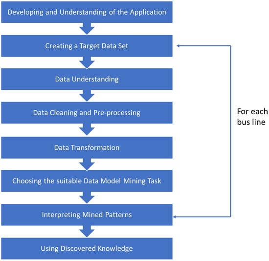
Figure 4. Proposed model.

4.1. Developing and Understanding of the Application

The objective was to obtain a model that can be used to predict and interpret real passenger demand given by EMT. For this company, it is critical to know the passenger demand that any bus line in the city may have on a given day. However, it is also critical to know why this demand is determined. In this way, the company will be able to make various decisions about the transport service, based on knowledge of what is expected to be happening and the factors and rules that will cause this demand.

In this work we focused on the analysis of bus line 1 in the afternoon schedule in the period January 2015–February 2017.

4.2. Creating a Target Data Set

The data of the mentioned bus line was provided by means of flat files (csv format).

These files contained events (each time a passenger inserts the ticket or travel card into the machine, an event is generated that includes timestamp information, bus ID, bus stop ID, bus direction and ticket type). Given the volume of the transactional data provided, we decided to use Big Data platforms. Therefore, these files were ingested in a Hadoop platform within a cluster, in order to have the data in a coherent and correctly integrated way to proceed with its subsequent analysis. For this, Hive was used, through which the input data from csv files were inserted into our Hadoop database. Spark was also used, through which we were able to work with the data inserted in a Hadoop database in a parallel way.

The output variables are:

-

Date: Field that indicates the date formed by year, month and day (e.g., 20160101);

-

Passengers: number of passengers in the selected time slot.

4.3. Data Understanding

This is the second phase of the CRISP-DM process, which focuses on data collection and quality review. We focused on the analysis of bus line 1 in the afternoon schedule. We observed that November was the month with the highest average daily demand, while August was the month with the lowest average daily demand. On the other hand, Wednesday was the day with the highest demand and Sunday the day with the least passengers. The daily average number of passengers was 3066.

In Figure 5, the time series of the daily number of passengers in the afternoon is shown. The histogram on this variable is shown in Figure 6.

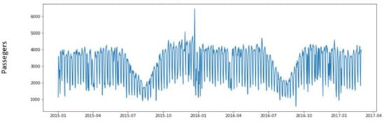
Figure 5. Daily number of passengers in the afternoon.

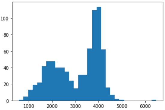
Figure 6. Histogram of passengers in the afternoon on bus line 1.

Once the different data sources are integrated, the variables are as follows:

-

Date: Field that indicates the date formed by year, month and day;

-

Month: indicates the month (e.g., January = 1);

-

Holiday; 1: yes, 0: no;

-

Day of week: indicates the day of week (e.g., Monday = 0);

-

Passengers: number of passengers.

4.4. Data Cleansing and Pre-Processing

This is the third stage of the KDD process, that focuses on the cleaning of target data and pre-processing. To do this, we represented line 1 by time slots and according to whether the day was a working day or weekend.

We noticed the presence of outliers or errors, since we found some travelers on daytime buses during nighttime hours, and on the other hand, travelers on night buses during daylight hours, so we removed these cases. For the night lines, we proceeded to maintain only the values that appear between 23 and 07 h.

Our database consisted of two sources: data from the buses, which we call “internal sources”, and all the data that do not come from the buses, which we call “external sources”.

First of all, we loaded the data in csv format or other formats to the HDFS system to later be inserted into our database. For this purpose, we developed two scripts in bash language that are responsible for loading the data from the cluster itself to the HDFS system. These scripts were divided according to the origin of the data, (internal sources versus external sources).

The internal sources are obtained from the bus machines that record the entry of passengers. Every time a passenger inserts the ticket or travel card into the machine, it generates a new entry in the database and is recorded as a new trip.

Finally, we obtained from http://www.calendarioslaborales.com (accessed on 28 February 2022) the holiday calendar of the Community of Madrid.

4.5. Data Transformation

This is the fourth stage of the KDD process that focuses on data transformation, so that algorithms can be easily implemented.

Some models are sensitive to the scale of the input data, so we transformed the scale by dividing the variable to be predicted by 5000. For all models except LSTM, we performed a one-hot encoding of the categorical variables day of week and month obtaining the following dummies:

-

day of week: Mon., Tue., Wed., Thu., Fri., Sat., Sun.;

-

month: Jan., Feb., March, April, May, June, July, Aug., Sept., Oct., Nov., Dec.

In the LSTM model, the categorical variables were processed using embedding layers.

Finally, we computed the lagged versions of the variables up to 5 days.

4.6. Choosing the Most Suitable ML Algorithm

At this stage of the KDD process, the appropriate data mining task is chosen. Once we performed the transformation of the data, we proceed to build the predictive system. For this, we developed different models with the aim of selecting the most accurate. Finally, the one selected for the project was the LSTM, which was developed in Keras [56]. The comparison of models is shown in Table 3.

Table 3. Comparison of models.

	Model	${\mathit{R}}^2\left(\mathbf{Test}\right)$
1	XGBoost	0.87
2	Random Forest	0.87
3	SVM (linear kernel)	0.88
4	SVM (polynomial kernel)	0.75
5	SVM (RBF kernel)	0.80
6	Shallow Dense Neural Network	0.80
7	LSTM	0.89

The blocks of an LSTM network contain different internal gates that control the flow of information (Figure 7), in such a way that when the gate has a value close to 0 the information does not flow through it, and when they have a value close to 1, information flows.

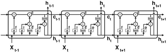
Figure 7. Illustration of an LSTM.

One of the gates (Forget Gate) is dedicated to forgetting, and controls the degree to which a value remains in the memory of the neuron, determining how much information about the past state should be discarded.

Where ft is the forget gate; σ is the sigmoid function; Wf is the forget gate weight matrix; x is the multiplication operator;

f_t = σ (W_f × [h_t−1, x_t] + b_f )

where f_t is the forget gate; σ is the sigmoid function; W_f is the forget gate weight matrix; h_t−1 is the output of the previous LSTM cell; x_t is the input; b_f is the bias for the gate.

The input gate, i_t, determines how much information about the current state of the network should be stored in the internal state.

i_t = σ(W_i × [h_t−1, x_t] + b_i)

The output gate, o_t, determines how much information from the current internal state should be sent to the external state.

o_t = σ(W_o × [h_t−1, x_t] + b_o)

The “tanh” node can be thought of as the activation function of the hidden layer, and its output is:

C_t = tanh(W_C × [h_t−1, x_t] + b_C)

In the final LSTM model, we used a configuration with 5 LSTM neurons, a window size of 5, a batch size of 32, and 2000 training epochs. Each of the categorical input variables (day of week and month) was processed by an embedding layer.

Finally, the dataset was divided into training dataset (80%, January 2015–September 2016) and test dataset (20%, September 2016–February 2017). In Figure 8, we can observe the day-by-day prediction of a range of days in the test set. We can see that the prediction fits quite well (R² train = 0.92, R² test = 0.89).

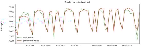
Figure 8. Zoom-in of the prediction in the test set. Dashed green: real value. Solid red: prediction.

4.7. Interpreting Mined Patterns

Once our ML model was built, which is a non-interpretable black box model in this phase, we obtain a surrogate rules model that allows interpretation from the business domain point of view.

To this purpose, we applied the steps from 1 to 6 of the algorithm explained in Section 3.2 for the LSTM model (chosen in the previous phase). Thus, we obtain the rules shown in Table 4.

Table 4. Surrogate rules obtained for the LSTM model.

Rule ID	Antecedent	Consequent
1	IF (Sat = 0) and (Sun = 0) and (holiday = 0) and (Jul = 0) and (Aug = 0) and (Sept = 0)	THEN prediction = 3907
2	IF (Sat = 0) and (Sun = 0) and (holiday = 0) and (Sept = 1)	THEN prediction = 3150
3	IF (Sat = 0) and (Sun = 0) and (holiday = 0) and (Jul = 1)	THEN prediction = 2694
4	IF (Sat = 1) and (y(−1) > 3110)	THEN prediction = 2438
5	IF (Sat = 0) and (Sun = 0) and (holiday = 1) and (Aug = 0)	THEN prediction = 1819
6	IF (Sat = 0) and (Sun = 0) and (Aug = 1)	THEN prediction = 1968
7	IF (Sat = 1) and (y(−1) ≤ 3110)	THEN prediction = 1627
8	IF (Sun = 1) and (y(−1) > 1832)	THEN prediction = 1874
9	IF (Sun = 1) and (y(−1) ≤ 1832)	THEN prediction = 1233

As discussed in Section 3.1, if we want to improve the interpretability of the variable number of passengers (prediction variable), we can represent it with its corresponding 2-tuple value. To this purpose, we applied steps 7 and 8 of the algorithm explained in Section 3.3. We first transformed this variable with the typical linear min-max transformation to represent it in the interval [0, 1], which is a necessary prior step for the transformation to a 2-tuple value (see Figure 3). The results of these transformations are shown in Table 5.

Table 5. 2-tuple representation of the predicted target variable.

Prediction	Prediction Min-Max Scale	Prediction 2-Tuple Representation
1233	0	Very Low
1627	0.1473448	(Low, −0.103)
1819	0.21914734	(Low, −0.031)
1832	0.22400898	(Low, −0.026)
1874	0.23971578	(Low, −0.01)
1968	0.27486911	(Low, 0.025)
2438	0.45063575	(Medium, −0.049)
2694	0.54637248	(Medium, 0.046)
3110	0.70194465	(High, −0.048)
3150	0.71690352	(High, −0.033)
3907	1	Very High

Once the predicted target variable was already represented linguistically, we proceed to replace the crisp values of this variable in the corresponding rules in a fuzzification process of this variable. After this process, we obtained the rules shown in Table 6. It should be noted that the use of the 2-tuple model allows the representation of the original variable in a linguistic but fully accurate way without loss of information.

Table 6. Surrogate rules obtained for the LSTM model with 2-tuple linguistic representation.

Rule ID	Antecedent	Consequent
1	IF (Sat = 0) and (Sun = 0) and (holiday = 0) and (Jul = 0) and (Aug = 0) and (Sept = 0)	THEN prediction = (Very High, 0)
2	IF (Sat = 0) and (Sun = 0) and (holiday = 0) and (Sept = 1)	THEN prediction = (High, −0.033)
3	IF (Sat = 0) and (Sun = 0) and (holiday = 0) and (Jul = 1)	THEN prediction = (Medium, 0.046)
4	IF (Sat = 1) and (y(−1) > (High, −0.048))	THEN prediction = (Medium, −0.049)
5	IF (Sat = 0) and (Sun = 0) and (holiday = 1) and (Aug = 0)	THEN prediction = (Low, −0.031)
6	IF (Sat = 0) and (Sun = 0) and (Aug = 1)	THEN prediction = (Low, 0.025)
7	IF (Sat = 1) and (y(−1) ≤ (High, −0.048))	THEN prediction = (Low, −0.103)
8	IF (Sun = 1) and (y(−1) > (Low, −0.026))	THEN prediction = (Low, −0.01)
9	IF (Sun = 1) and (y(−1) ≤ (Low, −0.026))	THEN prediction = (Very Low, 0)

We used time series, so the predicted variable itself was also used as an independent variable at earlier points in time. These independent variables were also replaced by their corresponding 2-tuple values to improve the linguistic interpretability of the rules.

4.8. Using Discovered Knowledge

This is the last and final step of the KDD process where the discovered knowledge has value for different use cases. In Section 4.6, we obtained an LSTM model that predicts passenger demand as can be seen in Figure 8 with good accuracy (R² train = 0.92, R² test = 0.89) and also as seen in Section 4.7 the model can be interpreted through rules from the business point of view with good precision (R² train = 0.95, R² test = 0.95). Therefore, we qualitatively know the reason for the prediction.

5. Discussion

We built an LSTM model that forecasts bus passenger demand with high accuracy. Then we applied the methodology explained in Section 3.3, constructing a surrogate tree and transforming it into a 2-tuple. The surrogate rules obtained for the LSTM model with 2-tuple linguistic are shown in Table 6 and can be interpreted as:

• Rule 1: very high demand. Days that are not summer days and are neither weekends nor holidays. That is, days when people go about their daily routine.
• Rule 2: high demand. Days in September that are neither weekends nor holidays. In Madrid, the demand for passengers increases in the month of September because most of the population is already working and the schools are starting the academic year.

Passenger demand will be medium for the following cases:

• Rule 3: Days in July that are neither weekends nor holidays. On those days, students do not have to attend classes and from the second fortnight onwards, some workers start their vacations. Therefore, passenger demand starts to decrease.
• Rule 4: Saturdays when passenger demand on the eve was very high. A large part of the population does not work on Saturday afternoons. On those days, public transport is usually used for leisure activities, so passenger demand is lower than on the eve.

Passenger demand will be low for the following cases:

• Rule 5: Holiday that are not weekends or days in August. It seems that during those holidays people prefer to stay at home or move to other areas.
• Rule 6. August days that are not weekends. In August many companies close and workers have to take mandatory vacations. In addition, students do not have to go to class, so passenger demand declines.
• Rule 7. Saturdays where passenger demand on the eve was high/medium. Same interpretation as in Rule 4.
• Rule 8. Sundays where passenger demand on the eve was not low or very low. The activities carried out by people in Madrid are similar on Saturdays and Sundays, but many street stores are closed on Sundays. For this reason, passenger demand on these two days is similar, with a lower demand on Sundays.

Passenger demand will be very low for the following case:

• Rule 9. Sundays where passenger demand on the eve was very low. Same interpretation as in Rule 8.

We emphasize that the 2-tuple model allowed us, on the one hand, a good linguistic interpretability of the LSTM model. On the other hand, it allowed us precision in the interpretation of the rules. For example, Rules 5, 6, 7 and 8 imply a low demand forecast but with different symbolic translation so that we can distinguish that some cases are lower than others.

6. Conclusions and Future Work

The problem raised in this article is one of the most important for smart cities, since they focus on being able to make their transport network more efficient and control it, through the prediction of bus passenger demand. Most of the machine learning algorithms that are used with time series for this purpose are called black box algorithms, that is, they have a good prediction but are not interpretable by humans. However, interpretability of the model is crucial for transparency, traceability, and auditability, especially in public resources allocation.

In the literature, we found works oriented to the prediction and understanding of the traffic flow and works that seek to make the recommendations on the transport fleet interpretable. As far as we know, there is no work specifically oriented to the problem of predictability and interpretability of public bus users like the work presented here.

We have built an LSTM algorithm which is able to predict passenger demand in the public transport network and has been empirically demonstrated with a use case. We used a large amount of data using internal and external sources.

Finally, it has been possible to be interpretable thanks to the surrogate model and 2-tuple fuzzy linguistic model. A fuzzy technique called 2-tuple model improved the linguistic interpretability of the generated XAI model without losing accuracy. We did not find in the literature the joint use of both approaches.

From the economic point of view, passenger demand forecasting can be used for an optimal planning of the resources, leading to energy and cost savings for the public transport company. Additionally, this methodology can be applied in future work to predict passenger demand for others types of transport (air, railway, marine).

References

- Spirin, I.; Zavyalov, D.; Zavyalova, N. Globalization and development of sustainable public transport systems. In Proceedings of the 16th International Scientific Conference Globalization and Its Socio-Economic Consequences, Rajecke Teplice, Slovakia, 5–6 October 2016; Volume 5, pp. 2076–2084. [Google Scholar]
- Li, W.; Sui, L.; Zhou, M.; Dong, H. Short-term passenger flow forecast for urban rail transit based on multi-source data. EURASIP J. Wirel. Commun. Netw. 2021, 2021, 9. [Google Scholar] [CrossRef]
- Schmidhuber, J. Deep Learning in Neural Networks: An Overview. Neural Netw. 2015, 61, 85–117. [Google Scholar] [CrossRef] [PubMed] [Green Version]
- LeCun, Y.; Bengio, Y.; Hinton, G. Deep learning. Nature 2015, 521, 436–444. [Google Scholar] [CrossRef] [PubMed]
- Hochreiter, S.; Schmidhuber, J. Long Short-Term Memory. Neural Comput. 1997, 9, 1735–1780. [Google Scholar] [CrossRef] [PubMed]
- Gers, F.A.; Schmidhuber, J.; Cummins, F. Learning to Forget: Continual Prediction with LSTM. Neural Comput. 2000, 12, 2451–2471. [Google Scholar] [CrossRef] [PubMed]
- Jiao, F.; Huang, L.; Song, R.; Huang, H. An Improved STL-LSTM Model for Daily Bus Passenger Flow Prediction during the COVID-19 Pandemic. Sensors 2021, 21, 5950. [Google Scholar] [CrossRef] [PubMed]
- Zadeh, L.A. The concept of a linguistic variable and its applications to approximate reasoning. Pt I. Inf. Sci. 1975, 8, 199–249. [Google Scholar] [CrossRef]
- Liu, H.; Ning, H.; Mu, Q.; Zheng, Y.; Zeng, J.; Yang, L.T.; Huang, R.; Ma, J. A review of the smart world. Future Gener. Comput. Syst. 2019, 96, 678–691. [Google Scholar] [CrossRef]
- Manibardo, E.L.; Laña, I.; Del Ser, J. Deep learning for road traffic forecasting: Does it make a difference? IEEE Trans. Intell. Transp. Syst. 2021, 1–25. Available online: https://ieeexplore.ieee.org/document/9447807 (accessed on 28 February 2022). [CrossRef]
- Cristóbal, T.; Padrón, G.; Quesada-Arencibia, A.; Alayón, F.; de Blasio, G.; García, C.R. Bus travel time prediction model based on profile similarity. Sensors 2019, 19, 2869. [Google Scholar] [CrossRef] [PubMed] [Green Version]
- Cobo, M.J.; López-Herrera, A.G.; Herrera-Viedma, E.; Herrera, F. SciMAT: A new science mapping analysis software tool. J. Am. Soc. Inf. Sci. Technol. 2012, 63, 1609–1630. [Google Scholar] [CrossRef]
- Lv, W.; Lv, Y.; Ouyang, Q.; Ren, Y. A Bus Passenger Flow Prediction Model Fused with Point-of-Interest Data Based on Extreme Gradient Boosting. Appl. Sci. 2022, 12, 940. [Google Scholar] [CrossRef]
- Jin, W.; Li, P.; Wu, W.; Wei, L. Short-Term Public Transportation Passenger Flow Forecasting Method Based on Multi-source Data and Shepard Interpolating Prediction Method. In International Conference on Man-Machine-Environment System Engineering; Springer: Singapore, 2018; pp. 281–294. [Google Scholar] [CrossRef]
- Ouyang, Q.; Lv, Y.; Ma, J.; Li, J. An LSTM-Based Method Considering History and Real-Time Data for Passenger Flow Prediction. Appl. Sci. 2020, 10, 3788. [Google Scholar] [CrossRef]
- Gummadi, R.; Edara, S.R. Prediction of passenger flow of transit buses over a period of time using artificial neural network. In Proceedings of the Third, International Congress on Information and Communication Technology, London, UK, 27–28 February 2018; Springer: Singapore, 2019; pp. 963–971. [Google Scholar] [CrossRef]
- Nagaraj, N.; Gururaj, H.L.; Swathi, B.H.; Hu, Y.-C. Passenger flow prediction in bus transportation system using deep learning. Multimed Tools Appl. 2022, 81, 12519–12542. [Google Scholar] [CrossRef] [PubMed]
- Zhai, H.; Tian, R.; Cui, L.; Xu, X.; Zhang, W. A novel hierarchical hybrid model for short-term bus passenger flow forecasting. J. Adv. Transp. 2020, 2020, 7917353. [Google Scholar] [CrossRef]
- Zou, L.; Shu, S.; Lin, X.; Lin, K.; Zhu, J.; Li, L. Passenger Flow Prediction Using Smart Card Data from Connected Bus System Based on Interpretable XGBoost. Wirel. Commun. Mob. Comput. 2022, 2022, 5872225. [Google Scholar] [CrossRef]
- Liu, L.; Chen, R.C. A novel passenger flow prediction model using deep learning methods. Transp. Res. Part C Emerg. Technol. 2017, 84, 74–91. [Google Scholar] [CrossRef]
- Chen, T.; Fang, J.; Xu, M.; Tong, Y.; Chen, W. Prediction of Public Bus Passenger Flow Using Spatial–Temporal Hybrid Model of Deep Learning. J. Transp. Eng. Part A Syst. 2022, 148, 04022007. [Google Scholar] [CrossRef]
- Wu, W.; Xia, Y.; Jin, W. Predicting bus passenger flow and prioritizing influential factors using multi-source data: Scaled stacking gradient boosting decision trees. IEEE Trans. Intell. Transp. Syst. 2020, 22, 2510–2523. Available online: https://ieeexplore.ieee.org/document/9284598 (accessed on 28 February 2022). [CrossRef]
- Liu, Y.; Lyu, C.; Liu, X.; Liu, Z. Automatic feature engineering for bus passenger flow prediction based on modular convolutional neural network. IEEE Trans. Intell. Transp. Syst. 2020, 22, 2349–2358. Available online: https://ieeexplore.ieee.org/document/9141203 (accessed on 28 February 2022). [CrossRef]
- Liu, W.; Tan, Q.; Wu, W. Forecast and early warning of regional bus passenger flow based on machine learning. Math. Probl. Eng. 2020, 2020, 6625435. [Google Scholar] [CrossRef]
- Tan, Q.; Ling, X.; Chen, M.; Lu, H.; Wang, P.; Liu, W. Statistical analysis and prediction of regional bus passenger flows. Int. J. Mod. Phys. B 2019, 33, 1950094. [Google Scholar] [CrossRef]
- Bai, Y.; Sun, Z.; Zeng, B.; Deng, J.; Li, C. A multi-pattern deep fusion model for short-term bus passenger flow forecasting. Appl. Soft Comput. 2017, 58, 669–680. [Google Scholar] [CrossRef]
- Han, Y.; Wang, C.; Ren, Y.; Wang, S.; Zheng, H.; Chen, G. Short-term prediction of bus passenger flow based on a hybrid optimized LSTM network. ISPRS Int. J. Geo-Inf. 2019, 8, 366. [Google Scholar] [CrossRef] [Green Version]
- Zhang, N.; Chen, H.; Chen, X.; Chen, J. Forecasting public transit use by crowdsensing and semantic trajectory mining: Case studies. ISPRS Int. J. Geo-Inf. 2016, 5, 180. [Google Scholar] [CrossRef] [Green Version]
- Luo, D.; Zhao, D.; Ke, Q.; You, X.; Liu, L.; Zhang, D.; Ma, H.; Zuo, X. Fine-grained service-level passenger flow prediction for bus transit systems based on multitask deep learning. IEEE Trans. Intell. Transp. Syst. 2020, 22, 7184–7199. Available online: https://ieeexplore.ieee.org/document/9126198 (accessed on 28 February 2022). [CrossRef]
- Wang, Y.; Currim, F.; Ram, S. Deep Learning of Spatiotemporal Patterns for Urban Mobility Prediction Using Big Data. Inf. Syst. Res. 2022. [Google Scholar] [CrossRef]
- Toqué, F.; Khouadjia, M.; Come, E.; Trepanier, M.; Oukhellou, L. Short & long term forecasting of multimodal transport passenger flows with machine learning methods. In Proceedings of the 2017 IEEE 20th International Conference on Intelligent Transportation Systems (ITSC), Yokohama, Japan, 16–19 October 2017; IEEE: Piscataway, NJ, USA; pp. 560–566. Available online: https://ieeexplore.ieee.org/document/8317939 (accessed on 28 February 2022).
- Zhai, H.; Cui, L.; Nie, Y.; Xu, X.; Zhang, W. A comprehensive comparative analysis of the basic theory of the short term bus passenger flow prediction. Symmetry 2018, 10, 369. [Google Scholar] [CrossRef] [Green Version]
- Minh, D.; Wang, H.X.; Li, Y.F.; Nguyen, T.N. Explainable artificial intelligence: A comprehensive review. Artif. Intell. Rev. 2021, 1–66. [Google Scholar] [CrossRef]
- Rawal, A.; Mccoy, J.; Rawat, D.B.; Sadler, B.; Amant, R. Recent Advances in Trustworthy Explainable Artificial Intelligence: Status, Challenges and Perspectives. IEEE Trans. Artif. Intell. 2021, 1, 1. Available online: https://www.computer.org/csdl/journal/ai/5555/01/09645355/1zc6Hmkb1xm (accessed on 28 February 2022). [CrossRef]
- Thakker, D.; Mishra, B.K.; Abdullatif, A.; Mazumdar, S.; Simpson, S. Explainable artificial intelligence for developing smart cities solutions. Smart Cities 2020, 3, 1353–1382. [Google Scholar] [CrossRef]
- Peijl, E.V.D.; Najjar, A.; Mualla, Y.; Bourscheid, T.J.; Spinola-Elias, Y.; Karpati, D.; Nouzri, S. Toward XAI & Human Synergies to Explain the History of Art: The Smart Photobooth Project. In Proceedings of the International Workshop on Explainable, Transparent Autonomous Agents and Multi-Agent Systems, Virtual Event, 3–7 May 2021; Springer: Cham, Switzerland, 2021; pp. 208–222. [Google Scholar]
- Corchado, J.; Chamoso, P.; Hernández, G.; Gutierrez, A.R.; Camacho, A.; González-Briones, A.; Pinto-Santos, F.; Goyenechea, E.; Garcia-Retuerta, D.; Alonso-Miguel, M.; et al. Deepint. net: A rapid deployment platform for smart territories. Sensors 2021, 21, 236. [Google Scholar] [CrossRef] [PubMed]
- Kostopoulos, G.; Panagiotakopoulos, T.; Kotsiantis, S.; Pierrakeas, C.; Kameas, A. Interpretable Models for Early Prediction of Certification in MOOCs: A Case Study on a MOOC for Smart City Professionals. IEEE Access 2021, 9, 165881–165891. Available online: https://ieeexplore.ieee.org/document/9646955 (accessed on 28 February 2022). [CrossRef]
- Barredo-Arrieta, A.; Laña, I.; Del Ser, J. What lies beneath: A note on the explainability of black-box machine learning models for road traffic forecasting. In Proceedings of the 2019 IEEE Intelligent Transportation Systems Conference (ITSC), Auckland, NZ, USA, 27–30 October 2019; IEEE: Piscataway, NJ, USA; pp. 2232–2237. Available online: https://ieeexplore.ieee.org/document/8916985 (accessed on 28 February 2022).
- Daoud, A.; Alqasir, H.; Mualla, Y.; Najjar, A.; Picard, G.; Balbo, F. Towards Explainable Recommendations of Resource Allocation Mechanisms in On-Demand Transport Fleets. In Proceedings of the International Workshop on Explainable, Transparent Autonomous Agents and Multi-Agent Systems, Virtual Event, 3–7 May 2021; Springer: Cham, Switzerland, 2021; pp. 97–115. [Google Scholar]
- Alonso, J.M.; Castiello, C.; Mencar, C. A bibliometric analysis of the explainable artificial intelligence research field. In Proceedings of the International Conference on Information Processing and Management of Uncertainty in Knowledge-Based Systems, Cádiz, Spain, 11–15 June 2018; Springer: Cham, Switzerland, 2018; pp. 3–15. [Google Scholar]
- Herrera, F.; Martínez, L. A 2-tuple fuzzy linguistic representation model for computing with words. IEEE Trans. Fuzzy Syst. 2000, 8, 746–752. Available online: https://ieeexplore.ieee.org/document/890332 (accessed on 28 February 2022).
- Marín Díaz, G.; Carrasco, R.A.; Gómez, D. RFID: A Fuzzy Linguistic Model to Manage Customers from the Perspective of Their Interactions with the Contact Center. Mathematics 2021, 9, 2362. [Google Scholar] [CrossRef]
- Bueno, I.; Carrasco, R.A.; Porcel, C.; Herrera-Viedma, E. Profiling clients in the tourism sector using fuzzy linguistic models based on 2-tuples. Procedia Comput. Sci. 2022, 199, 718–724. [Google Scholar] [CrossRef]
- Elshawi, R.; Al-Mallah, M.H.; Sakr, S. On the interpretability of machine learning-based model for predicting hypertension. BMC Med. Inform. Decis. Mak. 2019, 19, 146. [Google Scholar] [CrossRef] [PubMed] [Green Version]
- Bueno, I.; Carrasco, R.A.; Ureña, R.; Herrera-Viedma, E. A business context aware decision-making approach for selecting the most appropriate sentiment analysis technique in e-marketing situations. Inf. Sci. 2022, 589, 300–320. [Google Scholar] [CrossRef]
- Molnar, C. Interpretable Machine Learning; Lulu Press: Morrisville, NC, USA, 2020. [Google Scholar]
- Bologna, G. A simple convolutional neural network with rule extraction. Appl. Sci. 2019, 9, 2411. [Google Scholar] [CrossRef] [Green Version]
- Keneni, B.M.; Kaur, D.; Al Bataineh, A.; Devabhaktuni, V.K.; Javaid, A.Y.; Zaientz, J.D.; Marinier, R.P. Evolving rule-based explainable artificial intelligence for unmanned aerial vehicles. IEEE Access 2019, 7, 17001–17016. [Google Scholar] [CrossRef]
- Singh, N.; Singh, P.; Bhagat, D. A rule extraction approach from support vector machines for diagnosing hypertension among diabetics. Expert Syst. Appl. 2019, 130, 188–205. [Google Scholar] [CrossRef]
- Fernandez, A.; Herrera, F.; Cordon, O.; del Jesus, M.J.; Marcelloni, F. Evolutionary fuzzy systems for explainable artificial intelligence: Why, when, what for, and where to? IEEE Comput. Intell. Mag. 2019, 14, 69–81. Available online: https://ieeexplore.ieee.org/document/8610271 (accessed on 28 February 2022). [CrossRef]
- Da Costa FChaves, A.; Vellasco, M.M.B.; Tanscheit, R. Fuzzy rules extraction from support vector machines for multi-class classification. Neural Comput. Appl. 2013, 22, 1571–1580. [Google Scholar] [CrossRef]
- Yeganejou, M.; Dick, S.; Miller, J. Interpretable deep convolutional fuzzy classifier. IEEE Trans. Fuzzy Syst. 2019, 28, 1407–1419. [Google Scholar] [CrossRef]
- Viaña, J.; Cohen, K. Fuzzy-based, noise-resilient, explainable algorithm for regression. In Proceedings of the North American Fuzzy Information Processing Society Annual Conference, West Lafayette, IN, USA, 7–9 June 2021; Springer: Cham, Switzerland, 2021; pp. 461–472. [Google Scholar] [CrossRef]
- Shafique, U.; Qaiser, H. A comparative study of data mining process models (KDD, CRISP-DM and SEMMA). Int. J. Innov. Sci. Res. 2014, 12, 217–222. [Google Scholar]
- Chollet, F. Deep Learning with Python; Manning: Shelter Island, NY, USA, 2018. [Google Scholar]
Publisher’s Note: MDPI stays neutral with regard to jurisdictional claims in published maps and institutional affiliations. |
© 2022 by the authors. Licensee MDPI, Basel, Switzerland. This article is an open access article distributed under the terms and conditions of the Creative Commons Attribution (CC BY) license (https://creativecommons.org/licenses/by/4.0/).