Survival with Random Effect

Abstract

The article focuses on mortality models with a random effect applied in order to evaluate human mortality more precisely. Such models are called frailty or Cox models. The main assertion of the paper shows that each positive random effect transforms the initial hazard rate (or density function) to a new absolutely continuous survival function. In particular, well-known Weibull and Gompertz hazard rates and corresponding survival functions are analyzed with different random effects. These specific models are presented with detailed calculations of hazard rates and corresponding survival functions. Six specific models with a random effect are applied to the same data set. The results indicate that the accuracy of the model depends on the data under consideration.

1. Introduction

Survival function is one of the most important variables, and describes human mortality. This function is the main element of certain mortality models. Other human mortality characteristics can be easily calculated by using the expression of survival function. One of these characteristics is the force of mortality, also known as the hazard rate. The most well-known classical examples of hazard rate functions are Weibull and Gompertz hazard rate functions. These functions have already been analyzed by many researchers, including Juckett and Rosenberg [1] and Missov et al. [2], among others. However, in 1979, Vaupel [3] was the first to present the idea to apply the random variable, also known as frailty or random effect, to the hazard rate function. Now, such derived models are called frailty models or random effect models. The definition of Cox models may also be used; see Lai [4] and Wienke [5], for instance. Frailty models were considered to represent mortality more precisely compared to the standard models. Frailty models and their applications to specific data sets have been widely used and analyzed by Manton and Vaupel, who collaborated with Stallard, Yashin, Iachine and Begun [3,6,7,8], as well as by Butt and Haberman [9], Moger and Aalen [10], Hougaard [11], Finkelstein [12] and Pitacco [13,14]. The idea of frailty models was expanded, as mixed hazard models suggested the hazard rate to have a polynomial expression—see Spreeuw et al. [15]—whereas Assabil [16] analyzed frailty models with time-dependable random effects.

This article focuses on the initial idea of frailty models: multiplying the initial hazard rate function by the random effect yields a new hazard rate function. The rest of the paper is organized as follows: at the beginning, we describe the main definitions and formulas for model calculations, and we present the main assertion of the paper. In this assertion, we prove that each positive random effect transforms the initial absolutely continuous survival function to a new absolutely continuous survival function. Furthermore, well-known Gompertz and Weibull model modifications are analyzed with different random effects, including random variables with gamma, Poisson, geometric and discrete uniform distributions. Each frailty model includes calculations of the hazard rate and survival function expressions. At the end, six particular models with a random effect are applied to the same data set of Baltic states mortality in order to determine which model fits the real mortality the best.

2. Theoretical Background

2.1. Main Concepts

To describe the mortality of a population, we use the classical concepts presented, for instance, in the book by Pitacco et al. [17] (see pages 51–58) or in papers [18,19]. The most general quantity, describing mortality, is the survival function S. This function shows the probability of an individual living at least x years, i.e., $S\left(x\right)=\mathbb{P}(T>x),$ where T denotes the life duration of the newborn by assuming that T is an absolutely continuous non-negative random variable.

It follows from this that the following requirements hold for each survival function S:

$$\begin{array}{ccc}& \left(\mathrm{i}\right)& S\left(x\right)isnotincreasingforx\in [0,\infty );\hfill \\ & \left(\mathrm{ii}\right)& S\left(0\right)=1;\hfill \\ & \left(\mathrm{iii}\right)& S(\infty ):=\underset{x\to \infty }{lim}S\left(x\right)=0;\hfill \\ & \left(\mathrm{iv}\right)& S\left(x\right)isabsolutelycontinuousontheinterval[0,\infty ).\hfill \end{array}$$

According to the definition of absolute continuity, for an arbitrary $\epsilon >0$, there is $\delta >0$, such that, for every finite collection of pairwise disjoint intervals $\{(a_1,b_1),\dots (a_n,b_n)\}$ with

$$\sum _{k=1}^n(b_k-a_k)<\delta ,$$

it holds that

$$\sum _{k=1}^n(S\left(a_k\right)-S\left(b_k\right))<\epsilon .$$

Due to the fundamental theorem of Lebesgue integral calculus, the above requirements (i)–(iv) for function S are equivalent to the existence of a non-negative integrable function f under condition

$${\int }_0^{\infty }f\left(y\right)\mathrm{d}y=1$$

such that

$$S\left(x\right)={\int }_x^{\infty }f\left(y\right)\mathrm{d}y,x⩾0;$$

(1)

see Chapter 5 in [20], for instance. Usually, function f is called the density function of the life duration T. The Cantor ternary function (see, for instance, Chapter 2 in [20]) shows that all of the requirements (i)–(iv) for the function should remain in order for the Equation (1) to be correct.

Another function describing the behaviour of life duration T is the hazard rate function, or the force of mortality

$${\mu }_x=\frac{f\left(x\right)}{S\left(x\right)}=-\frac{S^{\prime }\left(x\right)}{S\left(x\right)}$$

(2)

defined for almost all $x\in [0,\infty )$, such that $S\left(x\right)>0$.

The last formula shows that, by knowing the force of mortality, the survival function’s values at each non-negative x can be calculated. Namely,

$$S\left(x\right)=exp\left\{-\underset{0}{\overset{x}{\int }}{\mu }_u\mathrm{d}u\right\}$$

(3)

for all x under condition $S\left(x\right)>0$.

The requirements (i)–(iv) and the already mentioned fundamental theorem of the Lebesgue integral calculus imply that function S is a survival function if and only if the Equation (3) holds for a non-negative integrable (on each finite interval $[0,B],0<B<b$) function $\mu :[0,b)\to [0,\infty )$ under condition

$${\int }_0^b{\mu }_u\mathrm{d}u=\infty ,$$

where $b=inf\{x⩾0:S(x)=0\}$.

Equations (2) and (3) show that both functions $\mu$ and S are equally important in describing survival, and that one function can be replaced by another. In this work, we will pay more attention to the force of mortality.

2.2. Random Effect

In this paper, we consider survival models with random effects. This means that we consider survival functions having forces of mortality of the special form, and we focus on this form.

In 1979, Vaupel, Manton and Stallard [21] presented the idea of analyzing the modified function of mortality force

$${\mu }_{x|Z}=Z{\mu }_x,$$

(4)

where Z is a random variable, and, in the mortality model, is called the random effect, also known as the frailty parameter for a group of individuals; see [22,23].

If the force of mortality has the Formula (4), then function

$$\widehat{S}\left(x\right)=\mathbb{E}\left(S^Z\left(x\right)\right)=\mathbb{E}\left(exp\left\{-Z{\int }_0^x{\mu }_u\mathrm{d}u\right\}\right)$$

(5)

should be a new survival function, and

$$\widehat{\mu }\left(x\right)=-\frac{{\widehat{S}}^{\prime }\left(x\right)}{\widehat{S}\left(x\right)}=-log{\left(\mathbb{E}\left(S^Z\left(x\right)\right)\right)}^{\prime }$$

(6)

should be a new force of mortality.

Function $\widehat{S}$ is a new survival function and $\widehat{\mu }$ is a new force of mortality in the case where $\widehat{S}$ satisfies the requirements (i)–(iv) or, equivalently, when function $\widehat{S}$ satisfies the equality of type (1). The statement below shows that, with minimal constraints on the random variable Z, the function $\widehat{S}$, defined by Formula (5), is a survival function.

Theorem 1.

Let $S=S\left(x\right)$ be a survival function with a force of mortality $\mu ={\mu }_x$, and let Z be a positive random variable. Then, function $\widehat{S}=\widehat{S}\left(x\right)$, defined by Equation (5), is a new survival function.

Proof. 

We will prove that function $\widehat{S}$ satisfies the equality of type (1). According to Definition (5), we obtain:

$$\begin{array}{cc}\hfill \widehat{S}\left(x\right)& =\mathbb{E}\left(S^Z\left(x\right)\right)={\int }_{[0,\infty )}{S}^z\left(x\right)\mathrm{d}{F}_Z\left(z\right)\hfill \\ \hfill & ={\int }_{[0,\infty )}exp\left\{-z{\int }_0^x{\mu }_u\mathrm{d}u\right\}\mathrm{d}{F}_Z\left(z\right)\hfill \end{array}$$

for each $x⩾0$, where $F_Z$ is a distribution function of the random effect Z.

Let us define two real numbers:

$$\begin{array}{cc}\hfill a& =sup\{x⩾0:S(x)=1\};\hfill \\ \hfill b& =inf\{x⩾0:S(x)=0\}.\hfill \end{array}$$

It is obvious that $\widehat{S}\left(x\right)=1$ if $x\in [0,a]$ and $\widehat{S}\left(x\right)=0$ if $x\in [b,\infty )$ in the case of finite b.

It remains for us to consider $x\in (a,b)$. For these x, we have that $0<S\left(x\right)<1$. Therefore, for $z⩾0$ and $h>0$, we have

$$\begin{array}{cc}\hfill \left|\frac{S^z(x+h)-S^z\left(x\right)}{h}\right|& =\frac{S^z\left(x\right)}{h}\left|\frac{S^z(x+h)}{S^z\left(x\right)}-1\right|\hfill \\ \hfill & =\frac{S^z\left(x\right)}{h}\left|exp\left\{-z{\int }_x^{x+h}{\mu }_u\mathrm{d}u\right\}-1\right|\hfill \\ \hfill & ⩽z{S}^z\left(x\right)\frac{1}{h}{\int }_x^{x+h}{\mu }_u\mathrm{d}u\hfill \\ \hfill & =z{S}^z\left(x\right)\frac{1}{h}log\frac{S\left(x\right)}{S(x+h)}.\hfill \end{array}$$

Since S is absolutely continuous, derivative $S^{\prime }\left(x\right)$ exists almost everywhere on interval $(a,b)$. If $S^{\prime }\left(x\right)$ exists, then

$$logS\left(x\right)-logS(x+h)⩽\left(1-\frac{S^{\prime }\left(x\right)}{S\left(x\right)}\right)h$$

for sufficiently small $h>0$, which implies that

$$\left|\frac{S^z(x+h)-S^z\left(x\right)}{h}\right|⩽z{S}^z\left(x\right)\left(1-\frac{S^{\prime }\left(x\right)}{S\left(x\right)}\right).$$

For $z⩾0$ and sufficiently small $h<0$, the same estimate can be derived analogously. In addition, it is obvious that integral

$${\int }_{[0,\infty )}z{S}^z\left(x\right)\mathrm{d}{F}_Z\left(z\right)$$

is finite if $x\in (a,b)$.

Therefore, due to the Lebesgue’s dominated convergence theorem, we have that

$$\begin{array}{cc}\hfill {\widehat{S}}^{\prime }\left(x\right)& ={\int }_{[0,\infty )}\underset{h\to \infty }{lim}\frac{S^z(x+h)-S^z\left(x\right)}{h}\mathrm{d}{F}_Z\left(z\right)\hfill \\ \hfill & ={\int }_{[0,\infty )}{\left(S^z\left(x\right)\right)}^{\prime }\mathrm{d}{F}_Z\left(z\right)\hfill \\ \hfill & =-{\mu }_x{\int }_{[0,\infty )}z{S}^z\left(x\right)\mathrm{d}{F}_Z\left(z\right)\hfill \end{array}$$

for almost all $x\in (a,b)$.

Function ${\mu }_x$ is non-negative bounded and integrable on interval $[a,B]$ with an arbitrary $a<B<b$, whereas function

$${\int }_{[0,\infty )}z{S}^z\left(x\right)\mathrm{d}{F}_Z\left(z\right)$$

is continuous on interval $(a,b)$.

Consequently, derivative ${\widehat{S}}^{\prime }\left(x\right)$ is integrable on the interval $[a,B]$ with $a<B<b$. For $x\in [0,\infty )$, let us define

$$\widehat{f}\left(x\right)=-{\widehat{S}}^{\prime }\left(x\right)1{\mathrm{I}}_{(a,b)}\left(x\right).$$

Using the Tonelli’s theorem, we obtain

$$\begin{array}{cc}\hfill \underset{0}{\overset{\infty }{\int }}\widehat{f}\left(x\right)\mathrm{d}x& =\underset{a}{\overset{b}{\int }}(-{\widehat{S}}^{\prime }\left(x\right))\mathrm{d}x=\underset{a}{\overset{b}{\int }}\left(\underset{[0,\infty )}{\int }z{\mu }_x{\mathrm{e}}^{-z\underset{0}{\overset{x}{\int }}{\mu }_u\mathrm{d}u}\mathrm{d}{F}_Z\left(z\right)\right)\mathrm{d}x\hfill \\ \hfill & =\underset{[0,\infty )}{\int }\left(\underset{a}{\overset{b}{\int }}\mathrm{d}\left(-{\mathrm{e}}^{-z\underset{0}{\overset{x}{\int }}{\mu }_u\mathrm{d}u}\right)\right)\mathrm{d}{F}_Z\left(z\right)\hfill \\ \hfill & =\underset{[0,\infty )}{\int }\left(S^z\left(a\right)-S^z\left(b\right)\right)\mathrm{d}{F}_Z\left(z\right)=1.\hfill \end{array}$$

(7)

Similarly, for $x\in (a,b)$,

$$\begin{array}{cc}\hfill \underset{x}{\overset{\infty }{\int }}\widehat{f}\left(y\right)\mathrm{d}y& =\underset{x}{\overset{b}{\int }}(-{\widehat{S}}^{\prime }\left(y\right))\mathrm{d}y=\underset{x}{\overset{b}{\int }}\left(\underset{[0,\infty )}{\int }z{\mu }_y{\mathrm{e}}^{-z\underset{0}{\overset{y}{\int }}{\mu }_u\mathrm{d}u}\mathrm{d}{F}_Z\left(z\right)\right)\mathrm{d}y\hfill \\ \hfill & =\underset{[0,\infty )}{\int }\left(\underset{x}{\overset{b}{\int }}\mathrm{d}\left(-{\mathrm{e}}^{-z\underset{0}{\overset{y}{\int }}{\mu }_u\mathrm{d}u}\right)\right)\mathrm{d}{F}_Z\left(z\right)\hfill \\ \hfill & =\underset{[0,\infty )}{\int }\left(S^z\left(x\right)-S^z\left(b\right)\right)\mathrm{d}{F}_Z\left(z\right)=\widehat{S}\left(x\right).\hfill \end{array}$$

It follows from this that

$$\begin{array}{c}\hfill \widehat{S}\left(x\right)={\int }_x^{\infty }\widehat{f}\left(y\right)\mathrm{d}y,x\in [0,\infty )\end{array}$$

for an integrable non-negative function with Property (7).

The last equality has the Formula (1). Consequently, the function $\widehat{S}$ is a new survival function. The theorem is proved. □

Remark 1.

The above theorem provides us a large set of survival functions with a random effect. A new survival function can be constructed from any survival function S that meets the requirements (i)–(iv) and any positive random effect Z. The few examples below show that the random effect preserves the absolute continuity of the initial survival function but significantly changes its type.

For instance, let us consider the exponential survival function

$$S\left(x\right)={\mathrm{e}}^{-0.01x},x⩾0.$$

According to the above theorem, function $\widehat{S}\left(x\right)=\mathbb{E}{S}^Z\left(x\right)$ is a new absolutely continuous survival function in the case of the random effect Z under condition $\mathbb{P}(Z>0)=1$.

In particular, if Z is uniformly distributed on the interval $[a,b]$ with $0⩽a<b<\infty$, then, for $x⩾0$

$$\widehat{S}\left(x\right)=\frac{1}{b-a}{\int }_a^b{\mathrm{e}}^{-0.01xz}\mathrm{d}z=\frac{100}{(b-a)x}\left({\mathrm{e}}^{-0.001ax}-{\mathrm{e}}^{-0.01bx}\right).$$

If the random effect Z has an exponential distribution with positive parameter $\lambda$

$$\mathbb{P}(Z⩽z)=\left(1-{\mathrm{e}}^{-\lambda z}\right)1{\mathrm{I}}_{[0,\infty )}\left(z\right),$$

then the function

$$\widehat{S}\left(x\right)=\lambda {\int }_0^{\infty }{\mathrm{e}}^{-(0.01x+\lambda )z}\mathrm{d}z=\frac{\lambda }{0.01x+\lambda },x⩾0,$$

is a Pareto-type survival function.

If the random effect Z has the Bernoulli distribution

$$\mathbb{P}(Z=1)=(1-p),\mathbb{P}(Z=2)=p,p\in (0,1),$$

then the function with random effect

$$\widehat{S}\left(x\right)={\mathrm{e}}^{-0.01x}(1-p)+{\mathrm{e}}^{-0.02x}p,x⩾0,$$

is a mixture of exponential survival functions.

If the random effect Z is distributed according to the shifted Poisson law with positive parameter $\lambda$, then

$$\mathbb{P}(Z=k)={\mathrm{e}}^{-\lambda }\frac{{\lambda }^{k-1}}{(k-1)!},k\in \mathbb{N},$$

and, consequently,

$$\widehat{S}\left(x\right)={\mathrm{e}}^{-\lambda }\sum _{k=1}^{\infty }{\left(S\left(x\right)\right)}^k\frac{{\lambda }^{k-1}}{(k-1)!}={\mathrm{e}}^{-0.01x}{\mathrm{e}}^{\lambda \left({\mathrm{e}}^{-0.01x}-1\right)},x⩾0.$$

Finally, if Z has the classical Peter and Paul distribution

$$\mathbb{P}(Z=2^k)=\frac{1}{2^k},k\in \mathbb{N},$$

then

$$\widehat{S}\left(x\right)=\sum _{k=1}^{\infty }\frac{1}{2^k}{\mathrm{e}}^{-\left(2^{k}x\right)/100},x⩾0,$$

is the infinite mixture of exponential survival functions.

Remark 2.

In the case of the positive integer valued random effect Z, the survival function $\mathbb{E}{S}^Z\left(x\right)$ is the survival function of a randomly stopped minimum of independent random variables, considered, for instance, in [24,25,26].

Namely, suppose that $\{T_1,T_2,\dots \}$ are independent copies of the life duration T. In case $\mathbb{P}(Z=1)=1$, we have that

$$\mathbb{E}{S}^Z\left(x\right)=\mathbb{P}(T_1>x).$$

If $\mathbb{P}(Z=2)=1$, then

$$\mathbb{E}{S}^Z\left(x\right)=\mathbb{P}(T_1>x)\mathbb{P}(T_2>x)=\mathbb{P}\left(min\{T_1,T_2\}>x\right).$$

If $\mathbb{P}(Z=3)=1$, then

$$\mathbb{E}{S}^Z\left(x\right)=\mathbb{P}\left(min\{T_1,T_2,T_3\}>x\right).$$

Finally, in the case of integer valued random effect Z such that $\mathbb{P}(Z\in \mathbb{N})=1$, we have

$$\mathbb{E}{S}^Z\left(x\right)=\mathbb{P}\left(min\{T_1,T_2,\dots ,T_Z\}>x\right),$$

if random effect Z and the collection of life durations $\{T_1,T_2,\dots \}$ are independent.

The proved theorem justifies the use of a random effect in demographics to find the expression of the mortality force that is as consistent as possible with data. We note that the random effect applies not only to the transformations of survival but also to other models used in various studies. For instance, in [27,28,29,30], models with random effects have been used in medical research, in [31,32,33,34,35,36], models with random effects are adapted for statistical analysis of certain problems and in [37,38], probabilistic objects with additional random effects are examined.

3. Several Models with Random Effect

According to Theorem 1, we can construct a new survival function that has a basic force of mortality ${\mu }_x$ and a positive random variable Z. In this section, we present several examples of popular survival functions and corresponding hazard rates. From each selected survival function, we construct new survival functions using well-known random effects. For each selected pair of a survival function and random effect, we find the analytical expression of the new survival function and the analytical formula of the corresponding hazard rate.

3.1. Gamma–Weibull Model

At the beginning, let us consider the Weibull force of mortality

$${\mu }_x=c{x}^n,x⩾0,$$

depending on two positive parameters c and n. By choosing a gamma distributed random variable $Z\sim \Gamma (k,\lambda )$ for a random effect, we obtain the gamma–Weibull model described in [39,40], among others.

The gamma distributed random variable $Z\sim \Gamma (k,\lambda )$ has the density

$$f_Z\left(x\right)=\frac{{\lambda }^k}{\Gamma \left(k\right)}{x}^{k-1}{\mathrm{e}}^{-\lambda x},x⩾0,$$

where k and $\lambda$ are positive parameters and $\Gamma \left(k\right)$ is the standard gamma function.

The information above implies the following expression of the gamma–Weibull survival function:

$$\begin{array}{cc}\hfill {\widehat{S}}_{GW}\left(x\right)& =\mathbb{E}\left({\mathrm{e}}^{-Z\underset{0}{\overset{x}{\int }}{\mu }_t\mathrm{d}t}\right)=\underset{0}{\overset{\infty }{\int }}{\mathrm{e}}^{-z\underset{0}{\overset{x}{\int }}c{t}^n\mathrm{d}t}\frac{{\lambda }^k}{\Gamma \left(k\right)}{z}^{k-1}{\mathrm{e}}^{-\lambda z}\mathrm{d}z\hfill \\ \hfill & =\frac{{\lambda }^k}{\Gamma \left(k\right)}\underset{0}{\overset{\infty }{\int }}{\mathrm{e}}^{-z\left(\underset{0}{\overset{x}{\int }}c{t}^n\mathrm{d}t+\lambda \right)}{z}^{k-1}\mathrm{d}z.\hfill \end{array}$$

By denoting $w=z\left(\underset{0}{\overset{x}{\int }}c{t}^{n}dt+\lambda \right)$, we obtain

$$\begin{array}{cc}\hfill {\widehat{S}}_{GW}\left(x\right)& =\frac{{\lambda }^k}{\Gamma \left(k\right)}\frac{1}{{\left(\underset{0}{\overset{x}{\int }}c{t}^n\mathrm{d}t+\lambda \right)}^k}\underset{0}{\overset{\infty }{\int }}{\mathrm{e}}^{-w}{w}^{k-1}\mathrm{d}w\hfill \\ \hfill & =\frac{{\lambda }^k}{{\left(\frac{c{x}^{n+1}}{n+1}+\lambda \right)}^k}={\left(\frac{c{x}^{n+1}}{(n+1)\lambda }+1\right)}^{-k}.\hfill \end{array}$$

It is clear that the obtained survival function has derivative

$${\widehat{S}}_{GW}^{\prime }\left(x\right)=-\frac{ck{x}^n}{\lambda }{\left(\frac{c{x}^{n+1}}{\lambda (n+1)}+1\right)}^{-k-1}.$$

Hence, by using Formula (6), we obtain the following force of mortality expression for the gamma–Weibull model

$${\widehat{\mu }}_x=-\frac{{\widehat{S}}_{GW}^{\prime }\left(x\right)}{{\widehat{S}}_{GW}\left(x\right)}=\frac{ck{x}^n}{\frac{c{x}^{n+1}}{n+1}+\lambda }.$$

(8)

3.2. Gamma–Gompertz Model

In the gamma–Gompertz model, it is assumed that the basic force of mortality has the Gompertz expression, i.e.,

$${\mu }_x=B{\mathrm{e}}^{\alpha x},x⩾0,$$

(9)

with positive parameters B and $\alpha$. This expression can be derived from the Gompertz-Makeham model (see [41,42,43,44], among others). It should be noted that the Gompetz force of mortality belongs to Perk’s family of hazard rate functions and assumes that mortality increases exponentially with age [45,46].

In the Gamma–Gompertz model, random effect Z has a gamma expression, identical to the one in the gamma–Weibull model described in Section 3.1. Hence, in order to find the expression of the model’s survival function, identical calculations can be used to those that were performed while analyzing the gamma–Weibull model. The only difference is that the expression in the integral $c{t}^n$ should be changed by Gompertz expression $B{e}^{\alpha t}$. After the detailed calculations, we obtain the following expressions

$$\begin{array}{cc}\hfill {\widehat{S}}_{G{G}_4}\left(x\right)& ={\left(1+\frac{B}{\alpha \lambda }({\mathrm{e}}^{\alpha x}-1)\right)}^{-k},\hfill \end{array}$$

$$\begin{array}{cc}\hfill {\widehat{S}}_{G{G}_4}^{\prime }\left(x\right)& =-k\frac{B}{\lambda }{\mathrm{e}}^{\alpha x}{\left(1+\frac{B}{\alpha \lambda }({\mathrm{e}}^{\alpha x}-1)\right)}^{-k-1},\hfill \\ \hfill {\widehat{\mu }}_x& =-\frac{{\widehat{S}}_{G{G}_4}^{\prime }\left(x\right)}{{\widehat{S}}_{G{G}_4}\left(x\right)}=\frac{k\frac{B}{\lambda }{\mathrm{e}}^{\alpha x}}{\left(1+\frac{B}{\alpha \lambda }({\mathrm{e}}^{\alpha x}-1)\right)}.\hfill \end{array}$$

(10)

We can see that the above survival function ${\widehat{S}}_{G{G}_4}$ and force of mortality ${\widehat{\mu }}_x$ depend on four parameters. In addition to this general case, a separate version of the gamma-Gompertz model with three parameters can be considered, which we obtain by supposing $k=\lambda$. It is obvious that, for the gamma-Gompertz model with three parameters, we have:

$$\begin{array}{c}\hfill {\widehat{S}}_{G{G}_3}\left(x\right)={\left(1+\frac{B}{\alpha \lambda }({\mathrm{e}}^{\alpha x}-1)\right)}^{-\lambda },{\widehat{\mu }}_x=\frac{B{\mathrm{e}}^{\alpha x}}{\left(1+\frac{B}{\alpha \lambda }({\mathrm{e}}^{\alpha x}-1)\right)}.\end{array}$$

(11)

3.3. Poisson-Gompertz Model

In the Poisson-Gompertz model, the force of the mortality function has the Gompertz expression (9), whereas random effect Z has the shifted Poisson distribution with parameter $\lambda >0$, i.e.,

$$\mathbb{P}(Z=k)={\mathrm{e}}^{-\lambda }\frac{{\lambda }^{k-1}}{(k-1)!},k\in \mathbb{N}=\{1,2,\dots \}.$$

In the case of the integer-valued random variable Z, the expression of the survival function (5) obtains the following form

$$\widehat{S}\left(x\right)=\sum _{k=1}^{\infty }\mathbb{P}(Z=k)exp\left\{-k{\int }_0^x{\mu }_t\mathrm{d}t\right\}.$$

(12)

Therefore, for the Poisson-Gompertz model, we obtain

$$\begin{array}{cc}\hfill {\widehat{S}}_{PG}\left(x\right)& ={\mathrm{e}}^{-\lambda }\sum _{k=1}^{\infty }\frac{{\lambda }^{k-1}}{(k-1)!}{\mathrm{e}}^{-kB{\int }_0^x{\mathrm{e}}^{\alpha t}\mathrm{d}t}\hfill \\ & =exp\left\{-\lambda -B{\int }_0^x{\mathrm{e}}^{\alpha t}\mathrm{d}t\right\}\sum _{k=1}^{\infty }\frac{1}{(k-1)!}{\left(\lambda {\mathrm{e}}^{-B{\int }_0^x{\mathrm{e}}^{\alpha t}\mathrm{d}t}\right)}^{k-1}\hfill \\ \hfill & =exp\left\{\frac{B}{\alpha }(1-{\mathrm{e}}^{\alpha x})+\lambda \left({\mathrm{e}}^{\frac{B}{\alpha }(1-{\mathrm{e}}^{\alpha x})}-1\right)\right\}\hfill \end{array}$$

with positive parameters $\alpha$, B and $\lambda$.

The Poisson-Gompertz model is not integrated into package MortalityLaws of $\mathcal{R}$. Hence, for the data analysis, the expression should be derived for the force of mortality of ${\widehat{S}}_{PG}$. For this survival function, we obtain

$$\begin{array}{cc}\hfill {\widehat{S}}_{PG}^{\prime }\left(x\right)& ={\widehat{S}}_{PG}\left(x\right)\left(\frac{B}{\alpha }{(1-{\mathrm{e}}^{\alpha x})}^{\prime }+\lambda {\left({\mathrm{e}}^{\frac{B}{\alpha }(1-{\mathrm{e}}^{\alpha x})}\right)}^{\prime }\right)\hfill \\ \hfill & =-{\widehat{S}}_{PG}\left(x\right)B{\mathrm{e}}^{\alpha x}\left(\lambda {\mathrm{e}}^{\frac{B}{\alpha }(1-{\mathrm{e}}^{\alpha x})}+1\right).\hfill \end{array}$$

Consequently, the force of mortality for the Poisson-Gompertz model is the following:

$${\widehat{\mu }}_x=B{\mathrm{e}}^{\alpha x}\left(\lambda {\mathrm{e}}^{\frac{B}{\alpha }(1-{\mathrm{e}}^{\alpha x})}+1\right).$$

(13)

3.4. Geometric-Gompertz Model

In the geometric-Gompertz model, the mortality force function has the Gompertz expression (9), and the random effect Z has the shifted geometric distribution, i.e.,

$$\mathbb{P}(Z=k)=p{(1-p)}^{k-1},k\in \mathbb{N}.$$

Since random variable Z is discrete, by using Equality (12), we obtain

$$\begin{array}{cc}\hfill {\widehat{S}}_{GEG}\left(x\right)& =\sum _{k=1}^{\infty }p{(1-p)}^{k-1}{\mathrm{e}}^{-k{\int }_0^{x}B{\mathrm{e}}^{\alpha t}\mathrm{d}t}=p{\mathrm{e}}^{-B{\int }_0^x{\mathrm{e}}^{\alpha t}\mathrm{d}t}\sum _{k=1}^{\infty }{\left((1-p){\mathrm{e}}^{-B{\int }_0^x{\mathrm{e}}^{\alpha t}\mathrm{d}t}\right)}^{k-1}\hfill \\ \hfill & =\frac{p{\mathrm{e}}^{\frac{B}{\alpha }(1-{\mathrm{e}}^{\alpha x})}}{1-(1-p){\mathrm{e}}^{\frac{B}{\alpha }(1-{\mathrm{e}}^{\alpha x})}}\hfill \end{array}$$

with parameters $\alpha >0$, $B>0$ and $p\in (0,1)$.

The geometric-Gompertz model is also not integrated into package MortalityLaws of $\mathcal{R}$. Hence, the expression should be derived for the force of the mortality function. We obtain that

$${\widehat{S}}_{GEG}^{\prime }\left(x\right)=-\frac{pB{\mathrm{e}}^{\alpha x}{\mathrm{e}}^{\frac{B}{\alpha }(1-{\mathrm{e}}^{\alpha x})}}{{\left(1-(1-p){\mathrm{e}}^{\frac{B}{\alpha }(1-{\mathrm{e}}^{\alpha x})}\right)}^2}.$$

$${\widehat{\mu }}_x=\frac{B{\mathrm{e}}^{\alpha x}}{1-(1-p){\mathrm{e}}^{\frac{B}{\alpha }(1-{\mathrm{e}}^{\alpha x})}}.$$

(14)

3.5. Discrete-Weibull Model

In the discrete-Weibull case, differently to Section 3.1, we suppose that the force of mortality has a Weibull expression with the modal age of death, i.e., we suppose that

$${\mu }_x=\frac{1}{\sigma }{\left(\frac{x}{M}\right)}^{\frac{M}{\sigma }-1}$$

with positive parameters M and $\sigma$.

Usually, the parameter M is called the modal age of death, because, at this age, the population has the largest number of deaths; for details, see [2,47,48,49,50].

In the discrete–Weibull model, random effect Z is supposed to be discrete with finite support. We consider the case where random effect Z acquires three different values $1,2,3$. More precisely, we consider the three-point-discrete-Weibull model with Z having distribution $\mathbb{P}(Z=1)=p,\mathbb{P}(Z=2)=q,\mathbb{P}(Z=3)=1-p-q,$ where $p,q\in [0,1]$ and $p+q⩽1$.

For the model under consideration, by using Expression (12), we obtain

$$\begin{array}{cc}\hfill {\widehat{S}}_{DW}\left(x\right)& =p{\mathrm{e}}^{-{\left(\frac{x}{M}\right)}^{M/\sigma }}+q{\mathrm{e}}^{-2{\left(\frac{x}{M}\right)}^{M/\sigma }}+(1-p-q){\mathrm{e}}^{-3{\left(\frac{x}{M}\right)}^{M/\sigma }}.\hfill \end{array}$$

Since

$$\begin{array}{cc}\hfill {\widehat{S}}_{DW}^{\prime }\left(x\right)& =-\frac{1}{\sigma }{\left(\frac{x}{M}\right)}^{M/\sigma -1}\left(p{\mathrm{e}}^{-{\left(\frac{x}{M}\right)}^{M/\sigma }}+2q{\mathrm{e}}^{-2{\left(\frac{x}{M}\right)}^{M/\sigma }}+3(1-p-q){\mathrm{e}}^{-3{\left(\frac{x}{M}\right)}^{M/\sigma }}\right),\hfill \end{array}$$

we derive that

$${\widehat{\mu }}_x=\frac{1}{\sigma }{\left(\frac{x}{M}\right)}^{M/\sigma -1}\frac{p{\mathrm{e}}^{-{\left(\frac{x}{M}\right)}^{M/\sigma }}+2q{\mathrm{e}}^{-2{\left(\frac{x}{M}\right)}^{M/\sigma }}+3(1-p-q){\mathrm{e}}^{-3{\left(\frac{x}{M}\right)}^{M/\sigma }}}{p{\mathrm{e}}^{-{\left(\frac{x}{M}\right)}^{M/\sigma }}+q{\mathrm{e}}^{-2{\left(\frac{x}{M}\right)}^{M/\sigma }}+(1-p-q){\mathrm{e}}^{-3{\left(\frac{x}{M}\right)}^{M/\sigma }}}.$$

(15)

We note that, when p is equal to 1 the discrete-Weibull force of mortality, (15) becomes the free Weibull force of mortality.

4. Data and Model Fitness

For the empirical data, the mortality of Lithuanian, Latvian and Estonian populations in years 2000–2017 was used. Data were taken from the Human Mortality Database. Every country will be analyzed separately. For simplicity purposes, unisex mortality data will be used, i.e., results for men and women will not be separated. The reason behind this choice is based on the law presented in the European Union in 2012, stating that insurance companies are obliged to use the same mortality tables for both men and women. Therefore, the choice of using combined mortality data simplifies the use of results in practice. For empirical data, values of survival function and central mortality data of ages 0–110 were used. For simplicity, data for ages older than 110 were not analyzed separately; therefore, they were added to the data of age 110. Empirical values were derived by calculating averages of years 2000–2017 for every age group. Part of the empirical data is shown in the Table 1 below.

Table 1. Empirical data table.

	Estonia		Latvia		Lithuania
Age	${\tilde{m}}_x$	$\tilde{S}\left(x\right)$	${\tilde{m}}_x$	$\tilde{S}\left(x\right)$	${\tilde{m}}_x$	$\tilde{S}\left(x\right)$
0	0.0045	1	0.0071	1	0.0058	1
1	0.0005	0.9954	0.0006	0.9929	0.0005	0.9942
2	0.0003	0.9949	0.0004	0.9923	0.0003	0.9936
3	0.0002	0.9946	0.0003	0.9918	0.0003	0.9933
4	0.0002	0.9944	0.0003	0.9915	0.0003	0.9930
5	0.0003	0.9941	0.0003	0.9912	0.0002	0.9927
6	0.0002	0.9938	0.0002	0.9909	0.0002	0.9925
7	0.0002	0.9936	0.0003	0.9906	0.0002	0.9923
8	0.0002	0.9934	0.0002	0.9904	0.0002	0.9920
9	0.0001	0.9933	0.0002	0.9901	0.0002	0.9918
10	0.0002	0.9931	0.0002	0.9899	0.0002	0.9916
11	0.0002	0.9930	0.0002	0.9897	0.0002	0.9915
12	0.0002	0.9928	0.0002	0.9895	0.0002	0.9913
13	0.0002	0.9926	0.0002	0.9892	0.0002	0.9911
14	0.0002	0.9924	0.0003	0.9890	0.0003	0.9908
15	0.0004	0.9922	0.0003	0.9887	0.0004	0.9905
16	0.0004	0.9918	0.0006	0.9884	0.0005	0.9901
17	0.0005	0.9914	0.0006	0.9878	0.0007	0.9896
18	0.0008	0.9909	0.0007	0.9873	0.0009	0.9889
19	0.0008	0.9901	0.0009	0.9866	0.0010	0.98802
20	0.0010	0.9893	0.001	0.9857	0.0011	0.9869
…	…	…	…	…	…	…
50	0.0068	0.9172	0.0083	0.8972	0.0084	0.8950
51	0.0074	0.9109	0.0088	0.8897	0.0088	0.8875
52	0.0079	0.9042	0.0097	0.8819	0.0097	0.8797
53	0.0085	0.8971	0.0104	0.8734	0.0103	0.8711
54	0.0091	0.8895	0.0113	0.8643	0.0109	0.8622
55	0.0100	0.8815	0.0120	0.8546	0.0119	0.8529
56	0.0105	0.8727	0.0129	0.8444	0.0123	0.8428
57	0.0115	0.8636	0.0136	0.8336	0.0133	0.8325
58	0.0121	0.8538	0.0145	0.8223	0.0141	0.8215
59	0.0131	0.8435	0.0162	0.8105	0.0153	0.8099
60	0.0144	0.8326	0.0167	0.7975	0.0163	0.7977
…	…	…	…	…	…	…
100	0.4641	0.0073	0.4873	0.0041	0.4799	0.0051
101	0.4966	0.0045	0.5187	0.0025	0.5109	0.0031
102	0.5291	0.0027	0.5500	0.0015	0.5414	0.0018
103	0.5614	0.0016	0.5808	0.0008	0.5711	0.0010
104	0.5932	0.0009	0.6110	0.0004	0.5998	0.0006
…	…	…	…	…	…	…
110+	0.7613	0.00001	0.7670	0.000007	0.7422	0.00001

In the case of an arbitrary survival function $S\left(x\right)$ with force of mortality ${\mu }_x$, the behaviour of this force of mortality function in age interval $[x,x+1)$ can be described by the central mortality rate

$$m_x=\frac{\underset{0}{\overset{1}{\int }}S(x+u){\mu }_{x+u}\mathrm{d}u}{\underset{0}{\overset{1}{\int }}S(x+u)\mathrm{d}u}=\frac{S\left(x\right)-S(x+1)}{\underset{0}{\overset{1}{\int }}S(x+u)\mathrm{d}u}$$

(16)

The central mortality rate is usually provided in statistics; therefore, in order to fix the empirical values of the mortality force, the following assumption is used: the force of mortality in age interval $[x,x+1)$ is constant, i.e. ${\mu }_{x+t}={\mu }_x$ for all $x\in {\mathbb{N}}_0=\{0,1,\dots \}$ and $t\in [0,1)$. This assumption implies that the central mortality rate for $x\in {\mathbb{N}}_0$ can be equated to the force of mortality, i.e., $m_x={\mu }_x,x\in N_0.$

The force of mortality is the main characteristic analyzed in this work. According to the above remarks, we suppose that the mean square error

$$MSE=\frac{{\displaystyle \sum _{x=1}^N}{(\tilde{m}\left(x\right)-\widehat{\mu }\left(x\right))}^2}{N},$$

describes the fitness of the chosen force of mortality to the empirical data, where $N=110$, $\tilde{m}\left(x\right)$ are values of the empirical central mortality rate, and $\widehat{\mu }\left(x\right)$ denotes the force of mortality function values of the selected mortality model. The smaller the mean square error, the better the similarity between the force of the mortality function and empirical data. In the next section, models with the smallest MSE will be chosen and will be considered as the most fit to approximate and forecast the mortality of respective populations.

5. Data Analysis and Discussion

In this section, we consider a set of different mortality models satisfying the conditions of Theorem 1 with a different force of mortality and random effect applied to it. We select force of mortality functions generated by random effects analyzed in Section 3. All selected models were applied to Lithuanian, Latvian and Estonian mortality data. For all countries, we find the parameters of the selected force of mortality functions for which the MSE, defined by Equation (16), is the smallest. All calculations were performed using package MortalityLaws of the statistical program R. This package has 28 mortality models and eight error functions integrated into it, which help to find the best parameters estimates. The results for every country with each model’s parameter estimates are provided in Figure 1, Figure 2 and Figure 3 and Table 2, Table 3 and Table 4 below.

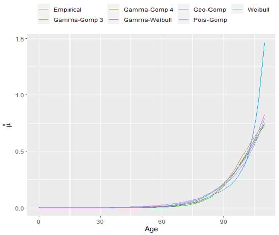
Figure 1. Mortality models with random effect applied to Lithuanian data.

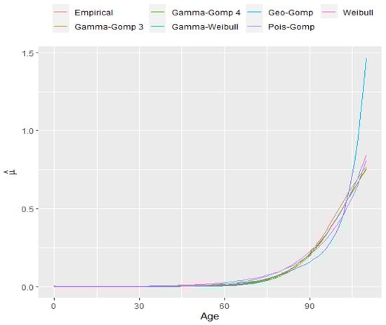
Figure 2. Mortality models with random effect applied to Latvian data.

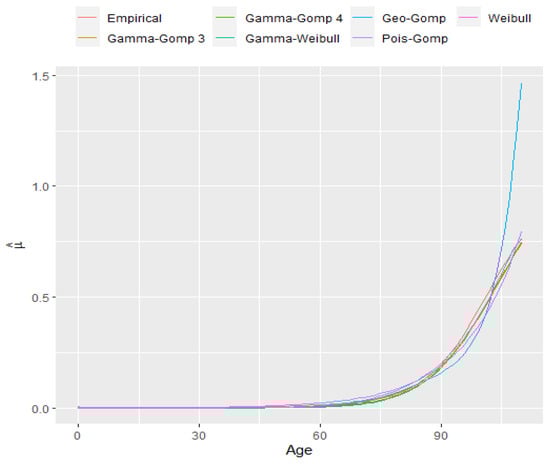
Figure 3. Mortality models with random effect applied to Estonian data.

Table 2. MSE for Lithuanian population.

Model	Mean Square Error (MSE)
Gamma-Gompertz with four parameters	0.0001820656
Gamma-Gompertz with three parameters	0.0001824057
Gamma-Weibull	0.0003312705
Weibull (discrete-Weibull with $p=1$)	0.0003361133
Poisson-Gompertz	0.0008037022
Geometric-Gompertz	0.01091893

Table 3. MSE for Latvian population.

Model	Mean Square Error (MSE)
Gamma-Gompertz with four parameters	0.0001455127
Gamma-Gompertz with three parameters	0.0001830891
Gamma-Weibull	0.0002027425
Weibull (discrete-Weibull with $p=1$)	0.0002679813
Poisson-Gompertz	0.0007349811
Geometric-Gompertz	0.01031875

Table 4. MSE for Estonian population.

Model	Mean Square Error (MSE)
Weibull (Discrete-Weibull with $p<1$)	0.0001198733
Gamma-Gompertz with three parameters	0.0001817575
Gamma-Gompertz with four parameters	0.0001832729
Gamma-Weibull	0.0001985111
Poisson-Gompertz	0.0006680722
Geometric-Gompertz	0.01013277

The best parameters for each model’s force of mortality function applied to Lithuanian data were:

• Gamma-Gompertz with four parameters; see (10):
  $\{B=5.136861\times {10}^{-7},\alpha =0.1250529,\lambda =1.320658,k=7.800965\}$;
• Gamma-Gompertz with three parameters; see (11):
  $\{B=3.028194\times {10}^{-6},\alpha =0.1250734,\lambda =7.798495\}$;
• Gamma-Weibull; see (8):
  $\{c=5.497963\times {10}^{-13},k=9347.058,\lambda =403176.2\times {10}^{12},n=6.752323\}$;
• Weibull (discrete-Weibull with $p=1$); see (15):
  $\sigma =10.38606,M=79.78316,p=1$;
• Poisson-Gompertz; see (13):
  $\{B=0.0003768185,\alpha =0.06951546,\lambda =5.637439\times {10}^{-7}\}$;
• Geometric-Gompertz; see (14):
  $\{\alpha =1.71132\times {10}^{-7},B=0.1451152,p=0.1467799\}.$

The best parameters for each model’s force of mortality function applied to Latvian data were:

• Gamma-Gompertz with four parameters; see (10):
  $\{B=0.003359441,\alpha =0.1071846,\lambda =2184.861,k=10.74998\}$;
• Gamma-Gompertz with three parameters; see (11):
  $\{B=6.45048\times {10}^{-6},\alpha =0.1171701,\lambda =9.04615\}$;
• Gamma-Weibull; see (8):
  $\{c=1.359224\times {10}^{-14},k=14.06893,\lambda =13115012,n=9.822215\}$;
• Weibull (discrete-Weibull with $p=1$); see (15):
  $\sigma =10.4192,M=79.16829,p=1$;
• Poisson-Gompertz; see (13):
  $\{B=0.0004160514,\alpha =0.06882173,\lambda =1.653197\times {10}^{-5}\}$;
• Geometric-Gompertz; see (14):
  $\{\alpha =1.71132\times {10}^{-7},B=0.1451152,p=0.1467799\}.$

The best parameters for each model’s force of mortality function applied to Estonian data are the following:

• Gamma-Gompertz with four parameters; see (10):
  $\{B=0.03077626,\alpha =0.1198032,\lambda =61698.92,k=8.989365\}$;
• Gamma-Gompertz with three parameters; see (11):
  $\{B=1.317173\times {10}^{-5},\alpha =0.1081533,\lambda =11.23144\}$;
• Gamma-Weibull; see (8):
  $\{c=0.9190396,k=0.004814763,\lambda =1.311606\times {10}^{-5},n=15.05727\}$;
• Weibull (discrete-Weibull with $p<1$); see (15):
  $\sigma =10.57929,M=89.5228,p=0.001071196,q=0.8634049$;
• Poisson-Gompertz; see (13):
  $\{B=0.0004160514,\alpha =0.06882173,\lambda =1.653197\times {10}^{-5}\}$;
• Geometric-Gompertz; see (14):
  $\{\alpha =1.71132\times {10}^{-7},B=0.1451152,p=0.1467799\}.$

Based on the results obtained, we made a conclusion that, for the Lithuanian and Latvian population, the gamma-Gompertz (with three or four parameters) models fit the empirical mortality data the best, whereas the discrete-Weibull model (with p < 1) is the best fit for the mortality of the Estonian population. As a result of a sufficiently small mean square error, all mortality force functions provided above are suitable to approximate the mortality of populations under consideration, except the geometric-Gompertz model, since the force of mortality of this model is similar to the step function, which is not usually used to describe the mortality of the real population. For the gamma-Gompertz model, the forecasted mortality is lower compared to statistics. Other analyses performed by Missov [51] and by Wang and Brown [52] also suggest that the gamma-Gompertz model increases the human life duration compared to actual statistics. Such a tendency is also observed in other Gompertz frailty models (see, for instance, the Poisson-Gompertz model and results obtained in [40] and [53]). For the discrete-Weibull model, a conclusion is made that the introduction of additional parameters into the force of mortality does not reduce the error of approximation of real data. It is important to note that previously described models cannot be considered as unambiguously best applicable for mortality forecasting, since the choice of model is highly dependent on the population that we are studying. This work only includes a small amount of mortality models. Therefore, the search for the unambiguously best applicable model for mortality forecasting remains one of the unsolved tasks for mathematicians and the life insurance market.

References

- Juckett, D.A.; Rosenberg, B. Comparison of the Gompertz and Weibull functions as descriptions for human mortality distributions and their intersections. Mech. Ageing Dev. 1993, 69, 1–31. [Google Scholar] [CrossRef]
- Missov, T.I.; Lenart, A.; Nemeth, L.; Canudas-Romo, V.; Vaupel, J.W. The Gompertz force of mortality in terms of the modal age at death. Demog. Res. 2015, 32, 1031–1048. [Google Scholar] [CrossRef]
- Vaupel, J.W. Inherited frailty and longevity. Demography 1988, 25, 277–287. [Google Scholar] [CrossRef]
- Lai, C.D. Constructions and applications of lifetime distributions. Appl. Stoch. Models Bus. Ind. 2013, 29, 127–140. [Google Scholar] [CrossRef]
- Wienke, A. Frailty models. In MPIDR Working Paper WP 2003–2032; Max Planck Institute for Demographic Research: Rostock, Germany, 2003. [Google Scholar]
- Manton, K.G.; Stallard, E.; Vaupel, J.W. Alternative Models for heterogeneity of mortality risks among the aged. J. Am. Stat. Assoc. 1986, 81, 635–644. [Google Scholar] [CrossRef]
- Manton, K.G. Changing concepts of morbidity and mortality in the elderly population. Milbank Mem. Fund Q. Health Soc. 1982, 60, 183–244. [Google Scholar] [CrossRef] [PubMed]
- Yashin, A.I.; Iachine, I.A.; Begun, A.Z.; Vaupel, J.W. Hidden frailty: Myths and reality. Doc. Trav. 2001, 34, 1–48. [Google Scholar]
- Butt, Z.; Haberman, S. Application of frailty-based mortality models using generalized linear models. ASTIN Bull. 2004, 34, 175–197. [Google Scholar] [CrossRef]
- Moger, T.A.; Aalen, O.O. Regression models for infant mortality data in Norwegian siblings, using a compound Poisson frailty distribution with random scale. Biostatistics 2008, 3, 577–591. [Google Scholar] [CrossRef] [PubMed][Green Version]
- Hougaard, P. Frailty models for survival data. Lifetime Data Anal. 1995, 1, 255–273. [Google Scholar] [CrossRef]
- Finkelstein, M.S. Lifesaving explains mortality decline with time. Math. Biosci. 2005, 196, 187–197. [Google Scholar] [CrossRef]
- Pitacco, E. From Halley to “frailty”: A review of survival models for actuarial calculations. Giornale dell’Istituto Italiano Degli Attuari. 2005. Available online: https://ssrn.com/abstract=741586 (accessed on 18 February 2022).
- Pitacco, E. High age mortality and frailty. Some remarks and hints for actuarial modelling. In Working Paper 2016/2019; CEPAR: Kensington, Australia, 2016; Available online: https://www.cepar.edu.au/publications/working-papers/high-age-mortality-and-frailty-some-remarks-and-hints-actuarial-modeling (accessed on 18 February 2022).
- Spreeuw, J.; Nielsen, J.P.; Jarner, S.F. A nonparametric visual test of mixed hazard models. SORT 2013, 1, 153–174. [Google Scholar]
- Assabil, S.E. Forecasting maternal mortality with modified Gompertz model. J. Adv. Math. Comput. Sci. 2019, 32, 1–7. [Google Scholar] [CrossRef][Green Version]
- Pitacco, E.; Denuit, M.; Haberman, S.; Olivieri, A. Modelling Longevity Dynamics for Pensions and Annuity Business; Oxford University Press: Oxford, UK, 2009. [Google Scholar]
- Gavrilov, L.A.; Gavrilova, N.S. The reliability theory of aging and longevity. J. Theor. Biol. 2001, 213, 527–545. [Google Scholar] [CrossRef]
- Henshaw, K.; Constantinescu, C.; Pamen, O.M. Stochastic mortality modelling for dependent coupled lives. Risks 2020, 8, 17. [Google Scholar] [CrossRef]
- Royden, H.L. Real Analysis; Macmillan Publishing Company: New York, NY, USA, 1969. [Google Scholar]
- Vaupel, J.M.; Manton, K.G.; Stallard, E. The impact of heterogeneity in individual frailty on the dynamics of mortality. Demography 1979, 6, 439–454. [Google Scholar] [CrossRef]
- Fulla, S.; Laurent, J.P. Mortality Fluctuations Modelling with a Shared Frailty Approach. Working Paper. 2008. Available online: http://laurent.jeanpaul.free.fr/ (accessed on 18 February 2022).
- Tuljapurkar, S.; Edwards, R.D. Variance in death and its implications for modelling and forecasting mortality. Demogr. Res. 2011, 24, 497–526. [Google Scholar] [CrossRef]
- Danilenko, S.; Šiaulys, J.; Stepanauskas, G. Closure properties of O-exponential distributions. Stat. Probab. Lett. 2018, 140, 63–70. [Google Scholar] [CrossRef]
- Ragulina, O.; Šiaulys, J. Randomly stopped minima and maxima with exponential-type distributions. Nonlinear Anal. Model. Control 2019, 24, 297–313. [Google Scholar] [CrossRef]
- Sprindys, J.; Šiaulys, J. Regularly distributed randomly stopped sum, minimum, and maximum. Nonlinear Anal. Model. Control 2020, 25, 509–522. [Google Scholar] [CrossRef]
- Alamer, A.A.; Almulhim, A.S.; Alrashed, A.A.; Abraham, I. Mortality, severity, and hospital admission among COVID-19 patients with ACEI/ARB use: A meta-analysis stratifying countries based on response to the first wave of the pandemic. Healthcare 2021, 9, 127. [Google Scholar] [CrossRef]
- Chen, J.-J.; Kuo, G.; Lee, T.H.; Yang, H.-Y.; Wu, H.H.; Tu, K.-H.; Tian, Y.-C. Incidence of mortality, acute kidney injury and graft loss in adult kidney transplant recipients with coronavirus disease 2019: Systematic review and meta-analysis. J. Clin. Med. 2021, 10, 5162. [Google Scholar] [CrossRef]
- Rivera-Izquierdo, M.; Pérez de Rojas, J.; Martínez-Ruiz, V.; Pérez-Gómez, B.; Sánchez, M.-J.; Khan, K.S.; Jiménez-Moleón, J.J. Obesity as a risk factor for prostate cancer mortality: A systematic review and dose-response meta-analysis of 280,199 patients. Cancers 2021, 13, 4169. [Google Scholar] [CrossRef]
- Turner, L.; Burbanks, A.; Cerasuolo, M. Mathematical insights into neuroendocrine transdifferentiation of human prostate cancer cells. Nonlinear Anal. Model. Control 2021, 5, 884–913. [Google Scholar] [CrossRef]
- Boucher, J.-P.; Turcotte, R. A longitudinal analysis of the impact of distance driven on the probability of car accidents. Risks 2020, 8, 91. [Google Scholar] [CrossRef]
- Hostiuc, S.; Diaconescu, I.; Rusu, M.C.; Negoi, I. Age estimation using the cameriere methods of open apices: A meta-analysis. Healthcare 2021, 9, 237. [Google Scholar] [CrossRef]
- Li, S.; Chen, J.; Chen, D. PQMLE of a partially linear, varying coefficient spatial autoregressive panel model with random effects. Symmetry 2021, 13, 2057. [Google Scholar] [CrossRef]
- Koroleva, E.; Jigeer, S.; Miao, A.; Skhvediani, A. Determinants affecting profitability of state-owned commercial banks: Case study of China. Risks 2021, 9, 150. [Google Scholar] [CrossRef]
- Młynarczyk, D.; Armero, C.; Gómez-Rubio, V.; Puig, P. Bayesian analysis of population health data. Mathematics 2021, 9, 577. [Google Scholar] [CrossRef]
- Zimon, G.; Appolloni, A.; Tarighi, H.; Shahmohammadi, S.; Daneshpou, E. Earnings management, related party transactions and corporate performance: The moderating role of internal control. Risks 2021, 9, 146. [Google Scholar] [CrossRef]
- Huang, Y.; Lu, Z.; Dai, W.; Zhang, W.; Wang, B. Remaining useful life prediction of cutting tools using an inverse Gaussian process model. Appl. Sci. 2021, 11, 5011. [Google Scholar] [CrossRef]
- Sazonov, I.; Grebennikov, D.; Meyerhans, A.; Bocharov, G. Markov chain-based stochastic modelling of HIV-1 life cycle in a CD4 T cell. Mathematics 2021, 9, 2025. [Google Scholar] [CrossRef]
- Klakattawi, H.S. The Weibull–Gamma distribution: Properties and applications. Entropy 2019, 21, 438. [Google Scholar] [CrossRef] [PubMed]
- Missov, T.I.; Lenart, A. Gompertz-Makeham life expectancies: Expressions and applications. Theor. Pop. Biol. 2013, 90, 29–35. [Google Scholar] [CrossRef] [PubMed]
- Burger, O.; Missov, T.I. Evolutionary theory of ageing and the problem of correlated Gompertz parameters. J. Theor. Biol. 2016, 408, 34–41. [Google Scholar] [CrossRef]
- Dotlačilová, P. Comparison of selected mortality models. In Proceedings of the 11th International Days of Statistics and Economics, Prague, Czech Republic, 14–16 September 2017; Vysoka Skola Ekonomicka: Prague, Czech Republic, 2017; pp. 324–337. [Google Scholar]
- Jarner, S.F.; Kryger, E.M. Modelling adult mortality in small populations: The SAINT model. ASTIN Bull. 2011, 41, 377–418. [Google Scholar]
- Saika, P.; Borah, M. A comparative study of parametric models of old-age mortality. Int. J. Sci. Res. 2014, 3, 406–410. [Google Scholar]
- Beard, R.E. Some aspects of theories of mortality, cause of death analysis, forecasting and stochastic processes. In Biological Aspects of Demography; Brass, W., Ed.; Taylor and Francis: London, UK, 1971; pp. 57–69. [Google Scholar]
- Pflaumer, P. Life table forecasting with Gompertz distribution. In JSM Proceedings, Social Statistics Section; American Statistical Association: Alexandria, VA, USA, 2007; pp. 3564–3571. [Google Scholar]
- Horiuchi, S.; Ouellette, N.; Cheung, S.L.K.; Robine, J.M. Modal age at death: Lifespan indicator in the era of longevity extension. Vienna Yearb. Pop. Res. 2013, 11, 37–69. [Google Scholar] [CrossRef]
- Rau, R.; Ebeling, M.; Peters, F.; Bohk-Ewald, C.; Missov, T.I. Where is the level of mortality plateau? In Living to 100, Society of Actuaries International Symposium; Society of Actuaries: Schaumburg, IL, USA, 2017. [Google Scholar]
- Cohen, J.E.; Bohk-Ewald, C.; Rau, R. Gompertz, Makeham and Siler models explain Taylor’s law in human mortality data. Demog. Res. 2018, 38, 773–842. [Google Scholar] [CrossRef]
- Romo, V.C. The modal age of death and the shifting mortality hypothesis. Demog. Res. 2008, 19, 1179–1204. [Google Scholar] [CrossRef]
- Missov, T.I. Gamma-Gompertz life expectancy at birth. Demogr. Res. 2013, 28, 59–270. [Google Scholar] [CrossRef]
- Wang, S.S.; Brown, R.L. A frailty model for projection of human mortality improvements. J. Actuar. Pract. 1998, 6, 1993–2006. [Google Scholar]
- Missov, T.I.; Vaupel, J.W. Mortality implications of morality plateaus. SIAM Rev. 2015, 57, 61–70. [Google Scholar] [CrossRef]
Publisher’s Note: MDPI stays neutral with regard to jurisdictional claims in published maps and institutional affiliations. |
© 2022 by the authors. Licensee MDPI, Basel, Switzerland. This article is an open access article distributed under the terms and conditions of the Creative Commons Attribution (CC BY) license (https://creativecommons.org/licenses/by/4.0/).