Gradient-Based Optimization Algorithm for Solving Sylvester Matrix Equation

Abstract

In this paper, we transform the problem of solving the Sylvester matrix equation into an optimization problem through the Kronecker product primarily. We utilize the adaptive accelerated proximal gradient and Newton accelerated proximal gradient methods to solve the constrained non-convex minimization problem. Their convergent properties are analyzed. Finally, we offer numerical examples to illustrate the effectiveness of the derived algorithms.

1. Introduction

Matrix equations are ubiquitous in signal processing [1], control theory [2], and linear systems [3]. Most time-dependent models accounting for the prediction, simulation, and control of real-world phenomena may be represented as linear or nonlinear dynamical systems. Therefore, the relevance of matrix equations within engineering applications largely explains the great effort put forth by the scientific community into their numerical solution. Linear matrix equations have an important role in the stability analysis of linear dynamical systems and the theoretical development of the nonlinear system. The Sylvester matrix equation was first proposed by Sylvester and produced from the research of relevant fields in applied mathematical cybernetics. It is a famous matrix equation that occurs in linear and generalized eigenvalue problems for the computation of invariant subspaces using Riccati equations [4,5,6]. The Sylvester matrix equation takes part in linear algebra [7,8,9], image processing [10], model reduction [11], and numerical methods for differential equations [12,13].

We consider the Sylvester matrix equation of the form

$$AX+XB=C,$$

(1)

where $A\in {\mathbb{R}}^{m\times m},B\in {\mathbb{R}}^{n\times n},C\in {\mathbb{R}}^{m\times n}$ are given matrices, and $X\in {\mathbb{R}}^{m\times n}$ is an unknown matrix to be solved. We discuss a special form of the Sylvester matrix equation, in which A and B are symmetric positive definite.

Recently, there has been a lot of discussion on the solution and numerical calculation of the Sylvester matrix equation. The standard methods for solving this equation are the Bartels–Stewart method [14] and the Hessenberg–Schur method [15], which are efficient for small and dense system matrices. When system matrices are small, the block Krylov subspace methods [16,17] and global Krylov subspace methods [18] are proposed. These methods use the global Arnoldi process, block Arnoldi process, or nonsymmetric block Lanczos process to produce low-dimensional Sylvester matrix equations. More feasible methods for solving large and sparse problems are iterative methods. When system matrices are large, there are some effective methods such as the alternating direction implicit (ADI) method [19], global full orthogonalization method, global generalized minimum residual method [20], gradient-based iterative method [21], and global Hessenberg and changing minimal residual with Hessenberg process method [22]. When system matrices are low-rank, the ADI method [23], block Arnoldi method [17], preconditioned block Arnoldi method [24], and extended block Arnoldi method [25] and its variants [26,27], including the global Arnoldi method [28,29] and extended global Arnoldi method [25], are proposed to obtain the low-rank solution.

The adaptive accelerated proximal gradient (A-APG) method [30] is an efficient numerical method for calculating the steady states of the minimization problem, motivated by the accelerated proximal gradient (APG) method [31], which has wide applications in image processing and machine learning. In each iteration, the A-APG method takes the step size by using a line search initialized with the Barzilai–Borwein (BB) step [32] to accelerate the numerical speed. Moreover, as the traditional APG method is proposed for the convex problem and its oscillation phenomenon slows down the convergence, the restart scheme has been used for speeding up the convergence. For more details, one can refer to [30] and the references therein.

The main contribution is to study gradient-based optimization methods such as the A-APG and Newton-APG methods for solving the Sylvester matrix equation through transforming this equation into an optimization problem by using Kronecker product. The A-APG and Newton-APG methods are theoretically guaranteed to converge to a global solution from an arbitrary initial point and achieve high precision. These methods are especially efficient for large and sparse coefficient matrices.

The rest of this paper is organized as follows. In Section 2, we transform this equation into an optimization problem by using the Kronecker product. In Section 3, we apply A-APG and Newton-APG algorithms to solve the optimization problem and compare them with other methods. In Section 4, we focus on the convergence analysis of the A-APG method. In Section 5, the computational complexity of these algorithms is analyzed exhaustively. In Section 6, we offer corresponding numerical examples to illustrate the effectiveness of the derived methods.

Throughout this paper, let ${\mathbb{R}}^{n\times m}$ be the set of all $n\times m$ real matrices. $I_n$ is the identity matrix of order n. If $A\in {\mathbb{R}}^{n\times n}$, the symbols $A^T$, $A^{-1}$, $\parallel A\parallel$ and $tr\left(A\right)$ express the transpose, the inverse, the 2-norm, and the trace of A, respectively. The inner product in matrix space $\mathbb{E}$ is $⟨x,y⟩=tr(x,y),\forall x,y\in \mathbb{E}$.

2. The Variant of an Optimization Problem

In this section, we transform the Sylvester equation into an optimization problem. We recall some definitions and lemmas.

Definition 1.

Let $Y=\left(y_{ij}\right)\in {\mathbb{R}}^{m\times n},Z\in {\mathbb{R}}^{p\times q}$, the Kronecker product of Y and Z be defined by

$$Y\otimes Z=\left[\begin{array}{cccc}{y}_{11}Z& y_{12}Z& \cdots & y_{1n}Z\\ y_{21}Z& y_{22}Z& \cdots & y_{2n}Z\\ ⋮& ⋮& ⋮& ⋮\\ y_{m1}Z& y_{m2}Z& \cdots & y_{mn}Z\end{array}\right].$$

Definition 2.

If $Y\in {\mathbb{R}}^{m\times n}$, then the straightening operator $vec:{\mathbb{R}}^{m\times n}⟶{\mathbb{R}}^{mn}$ of Y is

$$vec\left(Y\right)={(y_1^T,y_2^T,\dots ,y_n^T)}^T.$$

Lemma 1.

Let $Y\in {\mathbb{R}}^{l\times m},Z\in {\mathbb{R}}^{m\times n},W\in {\mathbb{R}}^{n\times k},$ then

$$vec\left(YZW\right)=(W^T\otimes Y)vec\left(Z\right).$$

From Lemma 1, the Sylvester Equation (1) can be rewritten as

$$(I_n\otimes A+B^T\otimes I_m)vec\left(X\right)=vec\left(C\right).$$

(2)

Lemma 2.

Let A be a symmetric positive matrix; solving the equation $Ax=b$ is equivalent to obtaining the minimum of $\phi \left(x\right)=x^{T}Ax-2b^{T}x$.

According to Lemma 2 and Equation (2), define

$$\overline{A}=(I_n\otimes A+B^T\otimes I_m),\overline{x}=vec\left(X\right),\overline{b}=vec\left(C\right).$$

Therefore, Equation (2) should be $\overline{A}\overline{x}=\overline{b}$. Obviously, if A and B are symmetric positive, then $\overline{A}$ is symmetric positive. The variant of the Sylvester Equation (2) reduces to the optimization problem:

$$\begin{array}{cc}\hfill min\phi \left(x\right)& =min\left\{{\overline{x}}^T\overline{A}\overline{x}-2{\overline{b}}^T\overline{x}\right\}\hfill \\ \hfill & =min\left\{vec{\left(X\right)}^T(I_n\otimes A+B^T\otimes I_m)vec\left(X\right)-2vec{\left(X\right)}^{T}vec\left(C\right)\right\}\hfill \\ \hfill & =min\left\{vec{\left(X\right)}^T·vec\left(AX\right)+vec{\left(X\right)}^T·vec\left(XB\right)-2vec{\left(X\right)}^T·vec\left(C\right)\right\}\hfill \\ \hfill & =min\left\{tr\left(X^{T}AX\right)+tr\left(X^{T}XB\right)-2tr\left(X^{T}C\right)\right\}.\hfill \end{array}$$

(3)

Using the calculation of the matrix differential from [33], we have the following propositions immediately.

Proposition 1.

If $A=\left(a_{ij}\right)\in {\mathbb{R}}^{m\times n},X=\left(x_{ij}\right)\in {\mathbb{R}}^{m\times n}$, then $\frac{\partial tr\left(A^{T}X\right)}{\partial X}=\frac{\partial tr\left(X^{T}A\right)}{\partial X}=A$.

Proposition 2.

If $A=\left(a_{ij}\right)\in {\mathbb{R}}^{m\times m},X=\left(x_{ij}\right)\in {\mathbb{R}}^{m\times n}$, then $\frac{\partial tr\left(X^{T}AX\right)}{\partial X}=AX+A^{T}X$.

Proposition 3.

If $B=\left(b_{ij}\right)\in {\mathbb{R}}^{n\times n},X=\left(x_{ij}\right)\in {\mathbb{R}}^{m\times n}$, then $\frac{\partial tr\left(X{X}^{T}B\right)}{\partial X}=XB+X{B}^T$.

Using Propositions 2 and 3, the gradient of the objective function (3) is

$$▽\phi \left(X\right)=AX+XB+A^{T}X+X{B}^T-2C.$$

(4)

By (4), the Hessian matrix is

$${▽}^2\phi \left(X\right)=A+A^T+B+B^T.$$

(5)

3. Iterative Methods

In this section, we will introduce the adaptive accelerated proximal gradient (A-APG) method and the Newton-APG method to solve the Sylvester equation. Moreover, we compare the A-APG and Newton-APG methods with other existing methods.

3.1. APG Method

The traditional APG method [31] is designed for solving the composite convex problem:

$$\underset{x\in \mathbb{H}}{min}H\left(x\right)=g\left(x\right)+f\left(x\right),$$

where $\mathbb{H}$ is the finite-dimensional Hilbert space equipped with the inner product $<·,·>$, g and f are both continuously convex, and $▽f$ has a Lipschitz constant L. Given initializations $x_1=x_0$ and $t_0=1$, the APG method is

$$\begin{array}{cc}\hfill t_k& =\left(\sqrt{4{(t-k-1)}^2+1}\right)/2,\hfill \\ \hfill Y_k& =X_k+\frac{t_{k-1}-1}{t_k}(X_k-X_{k-1}),\hfill \\ \hfill X_{k+1}& ={\mathrm{Prox}}_g^{\alpha }(Y_k-\alpha ▿f\left(Y_k\right)),\hfill \end{array}$$

where $\alpha \in (0,L]$ and the mapping ${\mathrm{Prox}}_g^{\alpha }(·):{\mathbb{R}}^n\mapsto {\mathbb{R}}^n$ is defined as

$${\mathrm{Prox}}_g^{\alpha }\left(x\right)=\underset{y}{argmin}\left\{g\left(y\right)+\frac{1}{2\alpha }{∥y-x∥}^2\right\}.$$

Since our minimization problem is linear, we choose the explicit scheme. The explicit scheme is a simple but effective approach for the minimization problem. Given an initial value $Y_0$ and the step ${\alpha }_k$, the explicit scheme is

$$Y_{k+1}=Y_k-{\alpha }_k▽\phi \left(Y_k\right),$$

(6)

where $Y_k$ is the approximation solution. The explicit scheme satisfies the sufficient decrease property using the gradient descent (GD) method.

Let $X_k$ and $X_{k-1}$ be the current and previous states and the extrapolation weight be $w_k$. Using the explicit method (6), the APG iterative scheme is

$$\begin{array}{cc}\hfill w_k& =k-2/k+1,\hfill \\ \hfill Y_k& =(1+w_k)X_k-w{X}_{k-1},\hfill \\ \hfill Y_{k+1}& =Y_k-{\alpha }_k▽\phi \left(Y_k\right).\hfill \end{array}$$

(7)

Together with the standard backtracking, we adopt the step size ${\alpha }_k$ when the following condition holds:

$$\phi \left(Y_k\right)-\phi \left(Y_{k+1}\right)\ge \eta {∥Y_{k+1}-Y_k∥}^2,$$

(8)

for some $\eta >0$.

Combining (7) and (8), the APG algorithm is summarized in Algorithm 1.

Algorithm 1 APG algorithm.

Require: $X_0,tol,{\alpha }_0,\eta >0,\beta \in (0,1)$, and $k=1$. 1: while the stop condition is not satisfied do 2:     Update $Y_k$ via Equation (7); 3:     if Equation (8) holds then 4:         $break$ 5:     else 6:         ${\alpha }_k=\beta {\alpha }_k$; 7:     Calculate $Y_{k+1}$ via (7); 8:     $k=k+1$.

3.2. Restart APG Method

Recently, an efficient and convergent numerical algorithm has been developed for solving a discretized phase-field model by combining the APG method with the restart technique [30]. Unlike the APG method, the restart technique involves choosing $X_{k+1}=Y_{k+1}$ whenever the following condition holds:

$$\phi \left(X_k\right)-\phi \left(Y_{k+1}\right)⩾\gamma {∥X_k-Y_{k+1}∥}^2,$$

(9)

for some $\gamma >0$. If the condition is not met, we restart the APG by setting $w_k=0$.

The restart APG method (RAPG) is summarized in Algorithm 2.

Algorithm 2 RAPG algorithm.

Require: $X_0,tol,{\alpha }_0,\eta >0,\gamma >0,\beta \in (0,1)$, and $k=1$. 1: while the stop condition is not satisfied do 2:     Calculate $Y_{k+1}$ by APG Algorithm 1; 3:     if Equation (9) holds then 4:         $X_{k+1}=Y_{k+1}$ and update ${\omega }_{k+1}$; 5:     else 6:         $X_{k+1}=X_k$ and reset ${\omega }_{k+1}=0$; 7:     $k=k+1$.

3.3. A-APG Method

In RAPG Algorithm 2, we can adaptively estimate the step size ${\alpha }_k$ by using the line search technique. Define

$$s_k:=X_k-X_{k-1},g_k:=▽\phi \left(X_k\right)-▽\phi \left(X_{k-1}\right).$$

We initialize the search step by the Barzilai–Borwein (BB) method, i.e.,

$$\begin{array}{c}\hfill {\alpha }_k={\displaystyle \frac{tr\left(s_k^T{s}_k\right)}{tr\left(s_k^T{g}_k\right)}}\mathrm{or}{\displaystyle \frac{tr\left(g_k^T{s}_k\right)}{tr\left(g_k^T{g}_k\right)}}.\end{array}$$

(10)

Therefore, we obtain the A-APG algorithm summarized in Algorithm 3.

Algorithm 3 A-APG algorithm.

Require: $X_0,tol,{\alpha }_0,\eta >0,\gamma >0,\beta \in (0,1)$, and $k=1$. 1: while the stop condition is not satisfied do 2:     Initialize ${\alpha }_k$ by BB step Equation (10); 3:     Update $X_{k+1}$ by RAPG Algorithm 2.

3.4. Newton-APG Method

Despite the fast initial convergence speed of the gradient-based methods, the tail convergence speed becomes slow. Therefore, we use a practical Newton method to solve the minimization problem. We obtain the initial value from A-APG Algorithm 3, and then choose the Newton direction as the gradient in the explicit scheme in RAPG Algorithm 2. Then we have the Newton-APG method shown in Algorithm 4.

Algorithm 4 Newton-APG algorithm.

Require: $X0,\alpha 0,\gamma >0,\eta >0,\beta \in (0,1),ϵ,tol$ and $k=1$. 1: Obtain the initial value from A-APG Algorithm 3 by the precision $ϵ$; 2: while the stop condition is not satisfied do 3:     Initialize ${\alpha }_k$ by BB step Equation (10); 4:     Update $X_{k+1}$ by RAPG Algorithm 2 using Newton direction.

3.5. Gradient Descent (GD) and Line Search (LGD) Methods

Moreover, we show gradient descent (GD) and line search (LGD) methods for comparing with the A-APG and Newton-APG methods. The GD and line search LGD methods are summarized in Algorithm 5.

Algorithm 5 GD and LGD algorithms.

Require: $X_0,tol,{\alpha }_0,\eta >0,\beta \in (0,1)$, and $k=1$. 1: while the stop condition is not satisfied do 2:     if the step size is fixed then 3:         Calculate $X_{k+1}$ via $X_{k+1}=X_k-\alpha ▽\phi \left(X_k\right)$ using GD; 4:     else 5:         Initialize ${\alpha }_k$ by BB step Equation (10); 6:         if Equation (8) holds then 7:            $break$ 8:         else 9:            ${\alpha }_k=\beta {\alpha }_k$; 10:         Calculate $X_{k+1}$ via $X_{k+1}$ via $X_{k+1}=X_k-\alpha ▽\phi \left(X_k\right)$ using LGD; 11:     $k=k+1$.

3.6. Computational Complexity Analysis

Further, we analyze the computational complexity of each iteration of the derived algorithms.

The computation of APG is mainly controlled by matrix multiplication and addition operations in three main parts. The iterative scheme needs $4m^{2}n+4m{n}^2+O\left(mn\right)$ computational complexity. The backtracking linear search needs $14m^{2}n+20n^{2}m+6n^3+O\left(mn\right)+O\left(n^2\right)$ computational complexity defined by Equation (8). The extrapolation needs $O\left(mn\right)$ computational complexity defined by the Equation (7). The total computational complexity is $18m^{2}n+24n^{2}m+6n^3+O\left(mn\right)+O\left(n^2\right)$ in Algorithm 1.

The computation of RAPG is mainly controlled by matrix multiplication and addition operations in four main parts. The iterative scheme needs $4m^{2}n+4m{n}^2+O\left(mn\right)$ computational complexity. The backtracking linear search defined by Equation (8) needs $14m^{2}n+20n^{2}m+6n^3+O\left(mn\right)+O\left(n^2\right)$ computational complexity. The extrapolation defined by Equation (7) needs $O\left(mn\right)$ computational complexity. The restart defined by Equation (9) needs $4m^{2}n+14n^{2}m+4n^3+O\left(mn\right)+O\left(n^2\right)$ computational complexity. The total computational complexity is $22m^{2}n+38n^{2}m+10n^3+O\left(mn\right)+O\left(n^2\right)$ in Algorithm 2.

The computation of A-APG is mainly controlled by matrix multiplication and addition operations in four main parts. The iterative scheme needs $4m^{2}n+4m{n}^2+O\left(mn\right)$ computational complexity. The BB step and the backtracking linear search defined by Equations (8) and (10) need $mn$, $4m^{2}n+4m{n}^2+6mn$, $2n^2(2m-1)+2n$, and $14m^{2}n+20n^{2}m+6n^3+O\left(mn\right)+O\left(n^2\right)$ computational complexity. The extrapolation defined by Equation (7) needs $O\left(mn\right)$ computational complexity. The restart defined by Equation (9) needs $4m^{2}n+14n^{2}m+4n^3+O\left(mn\right)+O\left(n^2\right)$ computational complexity. The total computational complexity is $26m^{2}n+46n^{2}m+10n^3+O\left(mn\right)+O\left(n^2\right)$ in Algorithm 3.

The computation of Newton-APG is mainly controlled by matrix multiplication and addition operations in four main parts, different from the A-APG method. The iterative scheme needs $8n^3+3n^2+O\left(n^2\right)+O\left(n^3\right)$ computational complexity. The BB step and the backtracking linear search defined by Equations (8) and (10) need $n^2$, $8n^3+6n^2$, $2n^2(2n-1)+2n$, and $10n^2(2n-1)+8n^3+3n^2+O\left(n^3\right)+O\left(n^2\right)$ computational complexity. The extrapolation defined by Equation (7) needs $O\left(n^2\right)$ computational complexity. The restart defined by Equation (9) needs $5n^2(2n-1)+n^2+O\left(n^3\right)$ computational complexity. The total computational complexity is $50n^3-10n^2+2n+O\left(n^2\right)+O\left(n^3\right)$ in Algorithm 4.

The computation of GD is mainly controlled by matrix multiplication and addition operations in Equations (4) and (6). It requires $mn(2m-1)$, $mn(2n-1)$, $mn(2m-1)$, $mn(2n-1)$ computational complexity to compute $AX$, $XB$, $A^{T}X$, $X{B}^T$. The total computational complexity is $4m^{2}n+4m{n}^2+O\left(mn\right)$ in Algorithm 5 using GD.

The computation of LGD is mainly controlled by matrix multiplication and addition operations in the calculation of s, g defined by Equation (8) and (10), and the calculation of GD, which require $mn$, $4m^{2}n+4m{n}^2+6mn$, $2n^2(2m-1)+2n$, $14m^{2}n+20n^{2}m+6n^3+O\left(mn\right)+O\left(n^2\right)$, and $4m^{2}n+4m{n}^2+O\left(mn\right)$, respectively. The total computational complexity is $22m^{2}n+32n^{2}m+6n^3+O\left(mn\right)+O\left(n^2\right)$ in Algorithm 5 using GD.

4. Convergent Analysis

In this section, we focus on the convergence analysis of A-APG Algorithm 3. The following proposition is required.

Proposition 4.

Let M be a bounded region that contains $\{\phi ⩽\phi \left(X_0\right)\}$ in ${\mathbb{R}}^{n\times n}$, then $▿\phi \left(X\right)$ satisfies the Lipschitz condition in M, i.e., there exists $L_M>0$ such that

$$∥▿\phi \left(X\right)-▿\phi \left(Y\right)∥⩽L_M∥X-Y∥forX,Y\in M.$$

Proof. 

Using the continuity of $▿\phi \left(X\right)$, note that

$$∥{▿}^2\phi \left(X\right)∥=∥(A+A^T)+(B+B^T)∥$$

defined by (5) is bounded. Then $▿\phi \left(X\right)$ satisfies the Lipschitz condition in M. □

In recent years, the proximal method based on the Bregman distance has been applied for solving optimization problems. The proximal operator is

$${\mathrm{Prox}}_{\phi }^{\alpha }\left(y\right):=\underset{y}{argmin}\{\phi \left(y\right)+\frac{1}{2\alpha }{∥X-X_k∥}^2\}.$$

Basically, given the current estimation $X_k$ and step size ${\alpha }_k>0$, update $X_{k+1}$ via

$$X_{k+1}={\mathrm{Prox}}_0^{\alpha }(X_k-{\alpha }_k▿\phi \left(X_k\right))=\underset{X}{argmin}\{\frac{1}{2{\alpha }_k}{∥X-(X_k-{\alpha }_k▿\phi \left(X_k\right)∥}^2\}.$$

(11)

Thus we obtain

$$\frac{1}{2{\alpha }_k}(X_{k+1}-(X_k-{\alpha }_k▿\phi \left(X_k\right)))=0,$$

which implies that

$$X_{k+1}=X_k-{\alpha }_k▿\phi \left(X_k\right).$$

This is exactly the explicit scheme in our algorithm.

4.1. Linear Search Is Well-Defined

Using the optimization from Equation (11), it is evident that

$$\begin{array}{cc}\hfill X_{k+1}& =\underset{X}{argmin}\{\frac{1}{2{\alpha }_k}{∥X-(X_k-{\alpha }_k▿\phi \left(X_k\right)∥}^2\}\hfill \\ \hfill & =\underset{X}{argmin}\{\frac{1}{2{\alpha }_k}{∥X-X_k∥}^2+⟨X-X_k,▿\phi \left(X_k\right)⟩\}\hfill \\ \hfill & =\underset{X}{argmin}\{\frac{1}{2{\alpha }_k}{∥X-X_k∥}^2+⟨X-X_k,▿\phi \left(X_k\right)⟩+\phi \left(X_k\right)\}.\hfill \end{array}$$

Then we obtain

$$\begin{array}{cc}\hfill \phi \left(X_k\right)& ⩾\frac{1}{2{\alpha }_k}{∥X_{k+1}-X_k∥}^2+⟨X_{k+1}-X_k,▿\phi \left(X_k\right)⟩+\phi \left(X_k\right)\hfill \\ \hfill & ⩾\phi \left(X_{k+1}\right)+\frac{1}{2{\alpha }_k}{∥X_k-X_{k+1}∥}^2-\frac{∥{▿}^2\phi \left(X\right)∥}{2}{∥X_k-X_{k+1}∥}^2\hfill \\ \hfill & ⩾\phi \left(X_{k+1}\right)+(\frac{1}{2{\alpha }_k}-\frac{L_M}{2}){∥X_k-X_{k+1}∥}^2,\hfill \end{array}$$

(12)

where the second inequality follows from Taylor expansion of $\phi \left(X_{k+1}\right)$. By Equation (12), set

$$0<{\alpha }_k<\overline{\alpha }:=min\{\frac{1}{L_M+2\eta },\frac{1}{L_M+2\gamma }\},$$

(13)

the conditions in linear search Equation (8) and non-restart Equation (9) are both satisfied. Therefore, the backtracking linear search is well-defined.

4.2. Sufficient Decrease Property

In this section, we show the sufficient decrease property of the sequence generated by A-APG Algorithm 3. If ${\alpha }_k$ satisfies the condition Equation (13), then

$$\phi \left(X_k\right)-\phi \left(Y_{k+1}\right)⩾{\rho }_1{∥X_k-Y_{k+1}∥}^2,$$

where ${\rho }_1=min\{\eta ,\gamma \}>0$. Since $\phi$ is a bounded function, then there exists ${\phi }^{*}$ such that $\phi \left(X_k\right)⩾{\phi }^{*}$ and $\phi \left(X_k\right)\to {\phi }^{*}$ as $k\to +\infty$. This implies

$${\rho }_1\sum _{k=0}^{\infty }{∥X_{k+1}-X_k∥}^2⩽\phi \left(X_0\right)-{\phi }^{*}<+\infty ,$$

which shows that

$$\underset{k\to +\infty }{lim}∥X_{k+1}-X_k∥=0.$$

4.3. Bounded Gradient

Define two sets ${\mathsf{\Omega }}_2=\{k:k=2\}$ and ${\mathsf{\Omega }}_1=N\backslash {\mathsf{\Omega }}_2$. Let $w_k=k-2/k+1$, for any $k\in {\mathsf{\Omega }}_2$, then $X_{k+1}=Y_{k+1}$ when $w_k=0$. There exists $\overline{w}=k_{max}-2/k_{max}+1\in [0,1)$ such that $w_k⩽\overline{w}$ as k increases. If $k\in {\mathsf{\Omega }}_1$, since

$$Y_{k+1}=\underset{X}{argmin}\left\{\frac{1}{2{\alpha }_k}{∥X-(Y_k-{\alpha }_k▿\phi \left(Y_k\right))∥}^2\right\},$$

we have

$$0=▿\phi \left(Y_k\right)+\frac{1}{{\alpha }_k}(Y_{k+1}-Y_k).$$

Thus,

$$▿\phi \left(Y_k\right)=\frac{1}{{\alpha }_k}(Y_k-X_{k+1}).$$

Note that $Y_k=(1+w_k)X_k-w_k{X}_{k-1}$, then

$$\begin{array}{cc}\hfill ∥▿\phi \left(Y_k\right)∥& =\frac{1}{{\alpha }_k}∥(1+w_k)X_k-w_k{X}_{k-1}-X_{k+1}∥\hfill \\ \hfill & =\frac{1}{{\alpha }_k}∥w_k(X_k-X_{k-1})+(X_k-X_{k+1})∥\hfill \\ \hfill & ⩽\frac{1}{{\alpha }_{min}}(\overline{w}∥X_k-X_{k-1}∥+∥X_k-X_{k+1}∥)\hfill \\ \hfill & =c_1(∥X_{k+1}-X_k∥+\overline{w}∥X_k-X_{k-1}∥),\hfill \end{array}$$

(14)

where $c_1=\frac{1}{{\alpha }_{min}}>0$.

If $k\in {\mathsf{\Omega }}_2$, then

$$X_{k+1}=\underset{X}{argmin}\left\{\frac{1}{2{\alpha }_k}{∥X-(X_k-{\alpha }_k▿\phi \left(X_k\right))∥}^2\right\},$$

which implies that

$$0=▿\phi \left(X_k\right)+\frac{1}{{\alpha }_k}(X_{k+1}-X_k).$$

Thus

$$∥▿\phi \left(X_k\right)∥=\frac{1}{{\alpha }_k}∥X_k-X_{k+1}∥⩽\frac{1}{{\alpha }_{min}}∥X_k-X_{k+1}∥=c_1\left(∥X_k-X_{k+1}∥\right),$$

(15)

Combining Equations (14) and (15), it follows that

$$∥▿\phi \left(X_k\right)∥⩽c_1(∥X_{k+1}-X_k∥+\overline{w}∥X_k-X_{k-1}∥).$$

4.4. Subsequence Convergence

As $\left\{X_k\right\}\in M$ is compact, there exists a subsequence $\left\{X_{k_j}\right\}\subset M$ and $X^{*}\in M$ such that $\underset{j\to +\infty }{lim}{X}_{k_j}=X^{*}$. Then $\phi$ is bounded, i.e., $\phi \left(X\right)>-\infty$ and $\phi$ keeps decreasing. Hence, there exists ${\phi }^{*}$ such that $\underset{k\to +\infty }{lim}\phi \left(X_k\right)={\phi }^{*}$. Note that

$$\phi \left(X_k\right)-\phi \left(X_{k+1}\right)⩾c_0{∥X_k-X_{k+1}∥}^2,k=1,2,\dots$$

(16)

Summation over k yields

$$c_0\sum _{k=0}^{\infty }{∥X_k-X_{k+1}∥}^2⩽\phi \left(X_0\right)-{\phi }^{*}<+\infty .$$

Therefore,

$$\underset{k\to +\infty }{lim}∥X_k-X_{k+1}∥=0.$$

Due to the property of the gradient, thus

$$\underset{j\to +\infty }{lim}∥▿\phi \left(X_{k_j}\right)∥=0.$$

Considering the continuity of $\phi$ and $▿\phi$, we have

$$\underset{j\to +\infty }{lim}\phi \left(X_{k_j}\right)=\phi \left(X^{*}\right),\underset{j\to +\infty }{lim}▿\phi \left(X_{k_j}\right)=▿\phi \left(X^{*}\right)=0,$$

which implies that $▿\phi \left(X^{*}\right)=0$.

4.5. Sequence Convergence

In this section, the subsequence convergence can be strengthened by using the Kurdyka–Lojasiewicz property.

Proposition 5.

For $\overline{x}\in$ dom $\partial \phi :=\{x:\partial \phi (x)\ne ⌀\}$, there exists $\eta >0$, an ϵ neighborhood of $\overline{x}$, and $\psi \in {\Psi }_{\eta }=\{\psi \in C[0,\eta )\cap C^{\prime }(0,\eta )$, where ψ is concave, $\psi \left(0\right)=0,{\psi }^{\prime }>0on(0,\eta )\}$ such that for all $x\in {\Gamma }_{\eta }(\overline{x},ϵ):U\cap \{x:\phi \left(\overline{x}\right)<\phi \left(x\right)<\phi \left(\overline{x}\right)+\eta \}$, we have

$${\psi }^{\prime }(\phi \left(x\right)-\phi \left(\overline{x}\right))∥▿\phi \left(x\right)∥⩾1.$$

Then we say $\phi \left(x\right)$ satisfies the Kurdyka–Lojasiewicz property.

Theorem 1.

Assume that Propositions 4 and 5 are met. Let $\left\{X_k\right\}$ be the sequence generated by A-APG Algorithm 3. Then, there exists a point $X^{*}\in M$ so that $\underset{k\to +\infty }{lim}{X}_k=X^{*}$ and $▿\phi \left(X^{*}\right)=0$.

Proof. 

Let $\omega \left(X_0\right)$ be the set of limiting points of the sequence $\left\{X_k\right\}$. Based on the boundedness of $\left\{X_k\right\}$ and the fact that $\omega \left(X_0\right)=\overline{{\cap }_{q\in N}{\cup }_{k>q}\left\{X_k\right\}}$, it follows that $\omega \left(X_0\right)$ is a non-empty and compact set. In addition, by Equation (16), we know that $\phi \left(X\right)$ is a constant on $\omega \left(X_0\right)$, denoted by ${\phi }^{*}$. If there exists some $k_0$ such that $\phi \left(X_{k_0}\right)={\phi }^{*}$, then for $\forall k>k_0$, we have $\phi \left(X_k\right)={\phi }^{*}$. Next, we assume that $\forall k,\phi \left(X_k\right)>{\phi }^{*}$. Therefore, for $\forall ϵ,\eta >0,\exists l>0$, for $\forall k>l$ we have $dist(\omega \left(X_0\right),X_k)⩽ϵ$ and ${\phi }^{*}<\phi \left(X_k\right)<{\phi }^{*}+\eta$ i.e., for $\forall X^{*}\in \omega \left(X_0\right),X\in {\Gamma }_{\eta }(X^{*},ϵ)$. Applying Proposition 5, for $\forall k>l$, we have

$${\psi }^{\prime }(\phi \left(X_k\right)-{\phi }^{*})∥▿\phi \left(X_k\right)∥⩾1.$$

Then

$${\psi }^{\prime }(\phi \left(X_k\right)-{\phi }^{*})⩾\frac{1}{c_1(∥X_k-X_{k-1}∥+\overline{w}∥X_{k-1}-X_{k-2}∥)}.$$

(17)

By the convexity of $\psi$, it is obvious that

$$\psi (\phi \left(X_k\right)-{\phi }^{*})-\psi (\phi \left(X_{k+1}\right)-{\phi }^{*})⩾{\psi }^{\prime }(\phi \left(X_k\right)-{\phi }^{*})(\phi \left(X_k\right)-\phi \left(X_{k+1}\right)).$$

(18)

Define

$${▵}_{p,q}=\psi (\phi \left(X_p\right)-{\phi }^{*})-\psi (\phi \left(X_q\right)-{\phi }^{*}),c=(1+\overline{w})c_1/c_0>0.$$

Combining with Equations (16)–(18), for $\forall k>l$, we obtain

$$\begin{array}{cc}\hfill {▵}_{k,k+1}& ⩾\frac{c_0{∥X_{k+1}-X_k∥}^2}{c_1(∥X_k-X_{k-1}∥+\overline{w}∥X_{k-1}-X_{k-2}∥)}\hfill \\ \hfill & ⩾\frac{{∥X_{k+1}-X_k∥}^2}{c(∥X_k-X_{k-1}∥+∥X_{k-1}-X_{k-2}∥)}.\hfill \end{array}$$

(19)

Applying the geometric inequality to Equation (19), thus

$$2∥X_{k+1}-X_k∥⩽\frac{1}{2}(∥X_k-X_{k-1}∥+∥X_{k-1}-X_{k-2}∥)+2c{▵}_{k,k+1}.$$

Therefore, for $\forall k>l$, summing up the above inequality for $i=l+1,\dots ,k$, we obtain

$$\begin{array}{cc}\hfill 2\sum _{i=l+1}^k∥X_{i+1}-X_i∥⩽& \frac{1}{2}\sum _{i=l+1}^k(∥X_i-X_{i-1}∥+∥X_{i-1}-X_{i-2}∥)+2c\sum _{i=l+1}^k{▵}_{i,i+1}\hfill \\ \hfill ⩽& \sum _{i=l+1}^k∥X_{i+1}-X_i∥+∥X_{l+1}-X_l∥+\frac{1}{2}∥X_l-X_{l-1}∥\hfill \\ \hfill & +2c{▵}_{l+1,k+1}.\hfill \end{array}$$

For $\forall k>l,\psi ⩾0$, it is evident that

$$\sum _{i=l+1}^k∥X_{i+1}-X_i∥⩽∥X_{l+1}-X_l∥+\frac{1}{2}∥X_l-X_{l-1}∥+2c\psi (\phi \left(X_l\right)-{\phi }^{*}),$$

which implies that

$$\sum _{k=1}^{\infty }∥X_{k+1}-X_k∥<\infty .$$

In the end, we have $\underset{k\to +\infty }{lim}{X}_k=X^{*}$. □

5. Numerical Results

In this section, we offer two corresponding numerical examples to illustrate the efficiency of the derived algorithms. All code is written in Python language. Denote iteration and error by the iteration step and error of the objective function. We take the matrix order “n” as 128, 1024, 2048, and 4096.

Example 1.

Let

$$A_1=\left(\begin{array}{cccccc}2& -1& & & & \\ -1& 2& -1& & & \\ & \ddots & \ddots & \ddots & \\ & & \ddots & \ddots & -1& \\ & & & -1& 2& \end{array}\right),B_1=\left(\begin{array}{cccccc}1& 0.5& & & & \\ 0.5& 1& 0.5& & & \\ & \ddots & \ddots & \ddots & \\ & & \ddots & \ddots & 0.5& \\ & & & 0.5& 1& \end{array}\right)$$

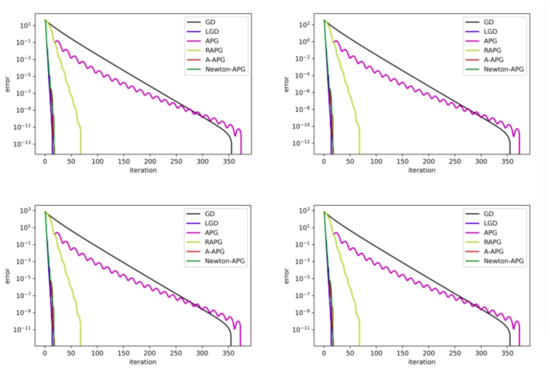
be tridiagonal matrices in the Sylvester Equation (1). Set the matrix $C_1$ as the identity matrix. The initial step size is 0.01, which is small enough to iterate. The parameters are ${\eta }_1=0.25,{\omega }_1=0.2$ taken from (0,1) randomly. Table 1 and Figure 1 show the numerical results of Algorithms 1–5. It can be seen that the LGD, A-APG, and Newton-APG Algorithms are more efficient than other methods. Moreover, the iteration step does not increase when the matrix order increases due to the same initial value. The A-APG method has higher error accuracy compared with other methods. The Newton-APG method takes more CPU time and fewer iteration steps than the A-APG method. The Newton method needs to calculate the inverse of the matrix, while it has quadratic convergence. From Figure 1, the error curves of the LGD, A-APG, and Newton-APG algorithms are hard to distinguish. We offer another example below.

Table 1. Numerical results for Example 1.

Algorithm	n	Iteration	Error	Time(s)
GD	128	356	1.13687 × 10${}^{-13}$	3.30
LGD	128	15	1.26477 × 10${}^{-12}$	0.27
APG	128	374	1.4353 × 10${}^{-12}$	4.31
RAPG	128	69	1.4353 × 10${}^{-12}$	1.45
A-APG	128	19	3.55271 × 10${}^{-14}$	0.38
Newton-APG	128	18	9.47438 × 10${}^{-11}$	0.48
CG	128	19	3.49364 × 10${}^{-14}$	0.42
GD	1024	356	1.02318 × 10${}^{-12}$	806
LGD	1024	15	1.06866 × 10${}^{-11}$	69
APG	1024	374	1.18803 × 10${}^{-11}$	1261
RAPG	1024	69	2.59774 × 10${}^{-11}$	367
A-APG	1024	19	2.84217 × 10${}^{-13}$	113
Newton-APG	1024	18	8.95682 × 10${}^{-10}$	144
CG	1024	19	3.37046 × 10${}^{-14}$	71
GD	2048	356	2.04636 × 10${}^{-12}$	6315
LGD	2048	15	2.13731 × 10${}^{-11}$	569
APG	2048	374	2.38742 × 10${}^{-11}$	9752
RAPG	2048	69	5.20686 × 10${}^{-11}$	2994
A-APG	2048	19	6.82121 × 10${}^{-13}$	926
Newton-APG	2048	18	8.95682 × 10${}^{-10}$	1015
CG	2048	19	3.34616 × 10${}^{-14}$	521
GD	4096	356	4.09273 × 10${}^{-12}$	66,155
LGD	4096	15	4.27463 × 10${}^{-11}$	4199
APG	4096	374	4.77485 × 10${}^{-11}$	71,636
RAPG	4096	69	1.04365 × 10${}^{-10}$	21,596
A-APG	4096	19	1.81899 × 10${}^{-12}$	6829
Newton-APG	4096	18	3.64571 × 10${}^{-9}$	7037
CG	4096	19	3.33322 × 10${}^{-14}$	3553

Figure 1. The error curves when n = 128, 1024, 2048, 4096 for Example 1.

Example 2.

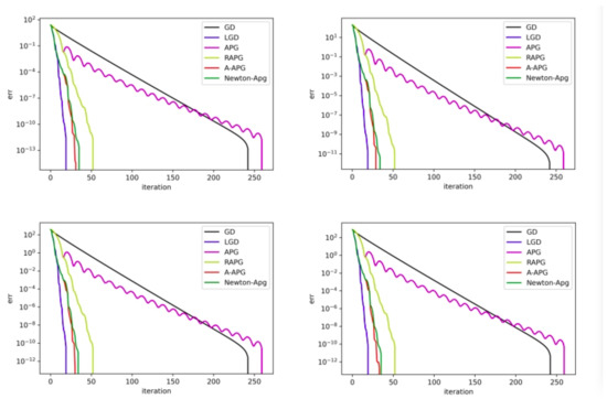
Let $A_2=A_1{A}_1^T,B_2=B_1{B}_1^T$ be positive semi-definite matrices in the Sylvester Equation (1). Set the matrix $C_2$ as the identity matrix. The initial step size is 0.009. The parameters are ${\eta }_2=0.28,{\omega }_2=0.25$ taken from (0,1) randomly. Table 2 and Figure 2 show the numerical results of Algorithms 1–5. It can be seen that the LGD, A-APG, and Newton-APG algorithms take less CPU time compared with other methods. Additionally, we can observe the different error curves of the LGD, A-APG, and Newton-APG algorithms from Figure 2.

Table 2. Numerical results for Example 2.

Algorithm	n	Iteration	Error	Time(s)
GD	128	243	1.63425 × 10${}^{-13}$	2.38
LGD	128	20	2.45137 × 10${}^{-12}$	0.47
APG	128	260	1.58096 × 10${}^{-12}$	4.51
RAPG	128	53	1.90781 × 10${}^{-12}$	1.46
A-APG	128	32	3.55271 × 10${}^{-15}$	0.78
Newton-APG	128	36	2.30926 × 10${}^{-13}$	1.26
CG	128	34	4.13025 × 10${}^{-14}$	0.79
GD	1024	243	1.3074 × 10${}^{-12}$	516
LGD	1024	20	1.89573 × 10${}^{-11}$	95
APG	1024	260	1.25056 × 10${}^{-11}$	835
RAPG	1024	53	1.51772 × 10${}^{-11}$	267
A-APG	1024	32	4.61569 × 10${}^{-14}$	181
Newton-APG	1024	36	4.20641 × 10${}^{-12}$	214
CG	1024	34	4.29936 × 10${}^{-14}$	92
GD	2048	243	2.6148 × 10${}^{-12}$	4129
LGD	2048	20	3.78577 × 10${}^{-11}$	814
APG	2048	260	2.48974 × 10${}^{-11}$	6507
RAPG	2048	53	3.03544 × 10${}^{-11}$	2193
A-APG	2048	32	2.27374 × 10${}^{-13}$	1622
Newton-APG	2048	36	8.52651 × 10${}^{-12}$	2125
CG	2048	34	4.22694 × 10${}^{-14}$	797
GD	4096	243	5.22959 × 10${}^{-12}$	29,859
LGD	4096	20	7.54881 × 10${}^{-11}$	6023
APG	4096	260	4.97948 × 10${}^{-11}$	48,238
RAPG	4096	53	6.07088 × 10${}^{-11}$	16,482
A-APG	4096	32	2.27374 × 10${}^{-13}$	12,896
Newton-APG	4096	36	7.95808 × 10${}^{-12}$	14,901
CG	4096	34	4.18275 × 10${}^{-14}$	5337

Figure 2. The error curves when n = 128, 1024, 2048, 4096 for Example 2.

Remark 1.

The difference of the iteration step in Examples 1 and 2 emerges due to the given different initial values. It can be seen that the LGD, A-APG, and Newton-APG algorithms have fewer iteration steps. Whether the A-APG method or Newton-APG yields fewer iteration steps varies from problem to problem. From Examples 1 and 2, we observe that the A-APG method has higher accuracy, although it takes more time and more iteration steps than the LGD method.

Remark 2.

Moreover, we compare the performance of our methods with other methods such as the conjugate gradient method (CG) in Table 1 and Table 2. We take the same initial values and set the error to 1 × 10${}^{-14}$. From Table 1 and Table 2, it can be seen that the LGD and A-APG methods are more efficient for solving the Sylvester matrix equation when the order n is small. When n is large, the LGD and A-APG methods nearly have a convergence rate with the CG method.

6. Conclusions

In this paper, we have introduced the A-APG and Newton-APG methods for solving the Sylvester matrix equation. The key idea is to change the Sylvester matrix equation to an optimization problem by using the Kronecker product. Moreover, we have analyzed the computation complexity and proved the convergence of the A-APG method. Convergence results and preliminary numerical examples have shown that the schemes are promising in solving the Sylvester matrix equation.

References

- Dooren, P.M.V. Structured Linear Algebra Problems in Digital Signal Processing; Springer: Berlin/Heidelberg, Germany, 1991. [Google Scholar]
- Gajic, Z.; Qureshi, M.T.J. Lyapunov Matrix Equation in System Stability and Control; Courier Corporation: Chicago, IL, USA, 2008. [Google Scholar]
- Corless, M.J.; Frazho, A. Linear Systems and Control: An Operator Perspective; CRC Press: Boca Raton, FL, USA, 2003. [Google Scholar]
- Stewart, G.W.; Sun, J. Matrix Perturbation Theory; Academic Press: London, UK, 1990. [Google Scholar]
- Simoncini, V.; Sadkane, M. Arnoldi-Riccati method for large eigenvalue problems. BIT Numer. Math. 1996, 36, 579–594. [Google Scholar]
- Demmel, J.W. Three methods for refining estimates of invariant subspaces. Computing 1987, 38, 43–57. [Google Scholar]
- Chen, T.W.; Francis, B.A. Optimal Sampled-Data Control Systems; Springer: London, UK, 1995. [Google Scholar]
- Datta, B. Numerical Methods for Linear Control Systems; Elsevier Inc.: Amsterdam, The Netherlands, 2004. [Google Scholar]
- Lord, N. Matrix computations. Math. Gaz. 1999, 83, 556–557. [Google Scholar]
- Zhao, X.L.; Wang, F.; Huang, T.Z. Deblurring and sparse unmixing for hyperspectral images. IEEE Trans. Geosci. Remote Sens. 2013, 51, 4045–4058. [Google Scholar]
- Obinata, G.; Anderson, B.D.O. Model Reduction for Control System Design; Springer Science & Business Media: London, UK, 2001. [Google Scholar]
- Bouhamidi, A.; Jbilou, K. A note on the numerical approximate solutions for generalized Sylvester matrix equations with applications. Appl. Math. Comput. 2008, 206, 687–694. [Google Scholar]
- Bai, Z.Z.; Benzi, M.; Chen, F. Modified HSS iteration methods for a class of complex symmetric linear systems. Computing 2010, 87, 93–111. [Google Scholar]
- Bartels, R.H.; Stewart, G.W. Solution of the matrix equation AX + XB = C. Commun. ACM 1972, 15, 820–826. [Google Scholar]
- Golub, G.H. A Hessenberg-Schur Method for the Problem AX + XB = C; Cornell University: Ithaca, NY, USA, 1978. [Google Scholar]
- Robbé, M.; Sadkane, M. A convergence analysis of GMRES and FOM methods for Sylvester equations. Numer. Algorithms 2002, 30, 71–89. [Google Scholar]
- Guennouni, A.E.; Jbilou, K.; Riquet, A.J. Block Krylov subspace methods for solving large Sylvester equations. Numer. Algorithms 2002, 29, 75–96. [Google Scholar]
- Salkuyeh, D.K.; Toutounian, F. New approaches for solving large Sylvester equations. Appl. Math. Comput. 2005, 173, 9–18. [Google Scholar]
- Wachspress, E.L. Iterative solution of the Lyapunov matrix equation. Appl. Math. Lett. 1988, 1, 87–90. [Google Scholar]
- Jbilou, K.; Messaoudi, A.; Sadok, H. Global FOM and GMRES algorithms for matrix equations. Appl. Numer. Math. 1999, 31, 49–63. [Google Scholar]
- Feng, D.; Chen, T. Gradient Based Iterative Algorithms for Solving a Class of Matrix Equations. IEEE Trans. Autom. Control 2005, 50, 1216–1221. [Google Scholar]
- Heyouni, M.; Movahed, F.S.; Tajaddini, A. On global Hessenberg based methods for solving Sylvester matrix equations. Comput. Math. Appl. 2019, 77, 77–92. [Google Scholar]
- Benner, P.; Kürschner, P. Computing real low-rank solutions of Sylvester equations by the factored ADI method. Comput. Math. Appl. 2014, 67, 1656–1672. [Google Scholar]
- Bouhamidi, A.; Hached, M.; Heyouni, M.J.; Bilou, K. A preconditioned block Arnoldi method for large Sylvester matrix equations. Numer. Linear Algebra Appl. 2013, 20, 208–219. [Google Scholar]
- Heyouni, M. Extended Arnoldi methods for large low-rank Sylvester matrix equations. Appl. Numer. Math. 2010, 60, 1171–1182. [Google Scholar]
- Agoujil, S.; Bentbib, A.H.; Jbilou, K.; Sadek, E.M. A minimal residual norm method for large-scale Sylvester matrix equations. Electron. Trans. Numer. Anal. Etna 2014, 43, 45–59. [Google Scholar]
- Abdaoui, I.; Elbouyahyaoui, L.; Heyouni, M. An alternative extended block Arnoldi method for solving low-rank Sylvester equations. Comput. Math. Appl. 2019, 78, 2817–2830. [Google Scholar]
- Jbilou, K. Low rank approximate solutions to large Sylvester matrix equations. Appl. Math. Comput. 2005, 177, 365–376. [Google Scholar]
- Liang, B.; Lin, Y.Q.; Wei, Y.M. A new projection method for solving large Sylvester equations. Appl. Numer. Math. 2006, 57, 521–532. [Google Scholar]
- Jiang, K.; Si, W.; Chen, C.; Bao, C. Efficient numerical methods for computing the stationary states of phase-field crystal models. SIAM J. Sci. Comput. 2020, 42, B1350–B1377. [Google Scholar]
- Beck, A.; Teboulle, M. A Fast Iterative Shrinkage-Thresholding Algorithm for Linear Inverse Problems. SIAM J. Imaging Sci. 2009, 2, 183–202. [Google Scholar]
- Bao, C.; Barbastathis, G.; Ji, H.; Shen, Z.; Zhang, Z. Coherence retrieval using trace regularization. SIAM J. Imaging Sci. 2018, 11, 679–706. [Google Scholar]
- Magnus, J.R.; Neudecker, H. Matrix Differential Calculus; John Willey & Sons: Hoboken, NJ, USA, 1999. [Google Scholar]
Publisher’s Note: MDPI stays neutral with regard to jurisdictional claims in published maps and institutional affiliations. |
© 2022 by the authors. Licensee MDPI, Basel, Switzerland. This article is an open access article distributed under the terms and conditions of the Creative Commons Attribution (CC BY) license (https://creativecommons.org/licenses/by/4.0/).