Border Irrigation Modeling with the Barré de Saint-Venant and Green and Ampt Equations

Abstract

In gravity irrigation, how water is distributed in the soil profile makes it necessary to study and develop methodologies to model the process of water infiltration and redistribution. In this work, a model is shown to simulate the advancing front in border irrigation based on the one dimensional equations of Barré de Saint-Venant for the surface flow and the equation of Green and Ampt for the flow in a porous medium. The solutions were obtained numerically using a finite difference Lagrangian scheme for the surface flow and the Raphson method for the subsurface flow. The model was validated with data obtained from the literature from an irrigation test and its predictive capacity was compared with another model and showed excellent results. The hydrodynamic parameters of the soil, necessary to obtain the optimal irrigation discharge, were obtained through the solution of the inverse problem using the Levenberg–Marquardt optimization algorithm. Finally, the results found here allow us to recommend that this model be used to design and model border irrigation, since the infiltration equation uses characteristic parameters of the physical soil.

1. Introduction

Gravity irrigation consists of pouring water at the head of a plot so that the water flows through a thalweg or tilted canal, such as a border strip or furrow, in the direction of the slope, to take advantage of the gravitational field and provide water to the roots of the cultivated plants, through the infiltration process, for their optimum development [1].

This irrigation method is the oldest and most used in agricultural plots worldwide, in about 90% [2,3,4]. Poor design, implementation, and management are generally responsible for inadequate irrigation, leading to water waste, salinization, and the pollution of surface and groundwater resources [5,6]. Typical border irrigation is showed in Figure 1, where it is observed what happens in the advance phase.

Different mathematical models simulate water flow in border irrigation, which differ in how the surface and subsurface flow description is approximated. As for surface flow, the developed models are mainly classified into four groups: the hydrodynamic wave model, the zero inertia model, the kinematic wave model, and the volume balance [7]. While the behavior of water movement through the soil is modeled by infiltration laws with potential forms such as the Kostiakov [8,9,10,11] or Kostiakov–Lewis [7,12,13,14,15] equation, and those using the one dimensional [5,16] and two dimensional [17,18] Richards’ equation, to describe the flow of water in the soil.

Using these models helps us to understand water movement in an irrigation event, which allows us to give pertinent recommendations for the efficient application of water on the plot [5]. Due to the heterogeneity of agricultural soils, the complexity characterizing its properties, as well as its effects on infiltration processes and surface water flow, the use of parameters that show representative conditions or behaviors for a specific area is required, so this study is governed by the hypothesis of the homogeneity of soil in a border.

The hydrodynamic wave model for the surface water flow is used in this work, therefore, the relationship between the width and depth of water in a border allows considering the equations corresponding to the runoff on a surface of infinite width [19]; the continuity equation is written as follows:

$$\frac{\partial \mathrm{h}}{\partial \mathrm{t}}+\frac{\partial \mathrm{q}}{\partial \mathrm{x}}+\frac{\partial \mathrm{I}}{\partial \mathrm{t}}=0$$

(1)

and the convenient form of the momentum equation is as follow:

$${\mathrm{h}}^2\frac{\partial \mathrm{q}}{\partial \mathrm{t}}+2\mathrm{h}\mathrm{q}\frac{\partial \mathrm{q}}{\partial \mathrm{x}}+\left(\mathrm{g}{\mathrm{h}}^3-{\mathrm{q}}^2\right)\frac{\partial \mathrm{h}}{\partial \mathrm{x}}+\mathrm{g}{\mathrm{h}}^3\left(\mathrm{J}-{\mathrm{J}}_{\mathrm{o}}\right)+\mathsf{\beta }\mathrm{q}\mathrm{h}\frac{\partial \mathrm{I}}{\partial \mathrm{t}}=0$$

(2)

where x is the main direction of movement of the water on the surface; t is the time, q(x,t) = U(x,t)h(x,t) is the rate per unit width of border o unit flow rate; U = U(x,t) is the average velocity in a cross section; h = h(x,t) is the water depth above the ground surface; Jo is the topographic slope of the border; J = J(x,t) is the friction slope related to a law of hydraulic resistance; g is the gravitational acceleration; ∂I(x,t)/∂t is the infiltration speed, that is, the volume of water infiltrated in a unit time per unit width and per unit length of border; I = I(x,t) is the volume infiltrated per unit area of soil surface or infiltrated depth; and β is a dimensionless parameter defined as β = U_IX/U, where U_IX is the projection in the direction of movement of the outflow velocity of the water mass due to infiltration, which is generally neglected.

Physical modeling of this phenomenon often suffers from numerical stability and convergence problems [20]. Possible instabilities of the numerical schemes can be attributed, at least partially, to the use of a hydraulic resistance law not compatible with equations, such as the Manning–Strickler law, therefore, the accepted law that relates the hydraulic variables q and h with the friction slope is the so called fractal law of hydraulic resistance [1]:

$$\mathrm{q}=\mathrm{k}\mathsf{\nu }{\left(\frac{{\mathrm{h}}^3\mathrm{J}\mathrm{g}}{{\mathsf{\nu }}^2}\right)}^{\mathrm{d}}$$

(3)

where ν is the coefficient of kinematic viscosity, k is a dimensionless factor that includes the effects of the roughness of the soil surface, and the exponent d is an exponent such that 1/2 ≤ d ≤ 1 in a way that d = 1/2 corresponds to the Chézy turbulent regime and d = 1 to the Poiseuille laminar regime.

Previous work uses the Manning–Strickler law established on a permanent regime to justify some experimental data. Manning left the power d = 1/2 fixed and recalculated the power of the hydraulic radius obtaining approximately 2/3. If this value of the power of the hydraulic radius is taken in the fractal law of hydraulic resistance 3d − 1 = 2/3, the value of the power of the friction slope is d = 5/9 [1], which recalculates the value of the Manning roughness coefficient as n = ν^1/9/kg^5/9.

For the vertical flow of water the Green and Ampt equation is used [21], which is established from the continuity equation and Darcy’s law with the following hypotheses: (a) the initial moisture profile in a soil column is uniform θ = θ₀; (b) the water pressure on the soil surface is hydrostatic: ψ = h ≥ 0, where h is the water depth; (c) there is a well defined wetting front characterized by a negative pressure: ψ = −h_f < 0, where hf is the suction at the wetting front; and (d) the region between the soil surface and the wetting front is completely saturated (plug flow): θ = θ_s and K = K_s, where K_s is the saturated hydraulic conductivity, that is, the value of the hydraulic conductivity of Darcy’s law corresponding to moisture saturated. The resulting ordinary differential equation is as follows:

$$\frac{\mathrm{d}\mathrm{I}}{\mathrm{d}\mathrm{t}}={\mathrm{K}}_{\mathrm{s}}\left(1+\frac{\left(\mathrm{h}+{\mathrm{h}}_{\mathrm{f}}\right)\left({\mathsf{\theta }}_{\mathrm{s}}-{\mathsf{\theta }}_0\right)}{\mathrm{I}}\right)$$

(4)

if the water depth is considered time independent, $\mathrm{h}={\overline{\mathrm{h}}}_{\mathrm{G}\mathrm{A}}$, Equation (4) is analytically integrated with the initial condition I = 0 on t = 0, resulting in:

$$\mathrm{I}={\mathrm{K}}_{\mathrm{s}}\mathrm{t}+\mathsf{\lambda }\ln \left(1+\frac{\mathrm{I}}{\mathsf{\lambda }}\right), \mathsf{\lambda }=\left({\overline{\mathrm{h}}}_{\mathrm{G}\mathrm{A}}+{\mathrm{h}}_{\mathrm{f}}\right)\left({\mathsf{\theta }}_{\mathrm{s}}-{\mathsf{\theta }}_0\right)$$

(5)

where ${\overline{\mathrm{h}}}_{\mathrm{G}\mathrm{A}}$ ≅ [4d/(5d + 1)]h_o is taken as the mean water depth and h_o = (ν²/gJ_o)^1/3(q₀/kν)^1/3d is the normal depth, with q₀ as the unitary discharge introduced to the border [22].

The correct design of the flow that must be applied to each border requires knowledge of the characteristics of the plots (length, moisture content, bulk density), the established crop, phenological stage and the water infiltrated to be applied, as well as the average parameters of the infiltration equation that is being used: Richards or Green and Ampt [23]. Recent studies have reported that it is possible to have high application efficiencies in gravity irrigation systems by applying the optimal flow at the entrance of the borders or furrows and maintaining a high uniformity coefficient in the plot called Christiansen uniformity coefficient [5,23].

The main objective of this study is to model the advance phase of border irrigation by coupling the hydrodynamic model of the Barré de Saint-Venant and Green and Ampt equations using a Lagrangian finite differences scheme and considering all the nodes in a calculation cell.

2. Materials and Methods

2.1. Numerical Solution

To solve the proposed coupling, a Lagrangian scheme is used in finite differences [9,24,25], based on a volume of control of moving cells, as shown in Figure 2.

The initial and boundary conditions are subject to the case of a closed border to avoid water loss by surface runoff outside the irrigation domain:

$$\begin{array}{l}\mathrm{q}\left(\mathrm{x},0\right)=0 ; \mathrm{h}\left(\mathrm{x},0\right)=0\\ \mathrm{q}\left(0,\mathrm{t}\right)={\mathrm{q}}_0 ; \mathrm{q}\left({\mathrm{x}}_{\mathrm{f}},\mathrm{t}\right)=0 ; \mathrm{h}\left({\mathrm{x}}_{\mathrm{f}},\mathrm{t}\right)=0\end{array}$$

(6)

where x_f(t) is the position of the advance front for the time t and q₀ the input discharge at the border entrance.

2.2. Solution Technique

The continuity equation (Equation (1)) for oblique cells is written as [9,24,25]:

$$\begin{array}{l}\left[\mathsf{\omega }{\mathrm{q}}_{\mathrm{L}}+\left(1-\mathsf{\omega }\right){\mathrm{q}}_{\mathrm{J}}\right]\mathsf{\delta }\mathrm{t}-\left[\mathsf{\omega }{\mathrm{q}}_{\mathrm{R}}+\left(1-\mathsf{\omega }\right){\mathrm{q}}_{\mathrm{M}}\right]\mathsf{\delta }\mathrm{t}\\ -\left[\mathsf{\phi }{\mathrm{h}}_{\mathrm{L}}+\left(1-\mathsf{\phi }\right){\mathrm{h}}_{\mathrm{R}}+\mathsf{\phi }{\mathrm{I}}_{\mathrm{L}}+\left(1-\mathsf{\phi }\right){\mathrm{I}}_{\mathrm{R}}\right]\left({\mathrm{x}}_{\mathrm{R}}-{\mathrm{x}}_{\mathrm{L}}\right)\\ +\left[\mathsf{\omega }\left({\mathrm{h}}_{\mathrm{R}}+{\mathrm{I}}_{\mathrm{R}}\right)+\left(1-\mathsf{\omega }\right)\left({\mathrm{h}}_{\mathrm{M}}+{\mathrm{I}}_{\mathrm{M}}\right)\right]\left({\mathrm{x}}_{\mathrm{R}}-{\mathrm{x}}_{\mathrm{M}}\right)\\ -\left[\mathsf{\omega }\left({\mathrm{h}}_{\mathrm{L}}+{\mathrm{I}}_{\mathrm{L}}\right)+\left(1-\mathsf{\omega }\right)\left({\mathrm{h}}_{\mathrm{J}}+{\mathrm{I}}_{\mathrm{J}}\right)\right]\left({\mathrm{x}}_{\mathrm{L}}-{\mathrm{x}}_{\mathrm{J}}\right)\\ +\left[\mathsf{\phi }{\mathrm{h}}_{\mathrm{J}}+\left(1-\mathsf{\phi }\right){\mathrm{h}}_{\mathrm{M}}+\mathsf{\phi }{\mathrm{I}}_{\mathrm{J}}+\left(1-\mathsf{\phi }\right){\mathrm{I}}_{\mathrm{M}}\right]\left({\mathrm{x}}_{\mathrm{M}}-{\mathrm{x}}_{\mathrm{J}}\right)=\mathrm{R}\mathrm{c}\end{array}$$

(7)

where, according to the Figure 2, the values of the dependent variables are known in the t_i timeline and the solution is sought in t_i+1, with the solution advancing in an increment of time δt = t_i+1 − t_i.

Due to the numerical instability presented at the first computation cells along the border, a discretization of the momentum equation (Equation (2)) was developed considering the follow hypothesis: (a) the derivatives in time are calculated as a Eulerian cell (rectangular), and (b) Equation (2) considers the average coefficients for the calculation of an average friction slope. With the above, the following form of discretized Equation (2) is proposed:

$$\begin{array}{l}2\overline{\mathrm{h}}\overline{\mathrm{q}}\left[\mathsf{\omega }\left({\mathrm{q}}_{\mathrm{R}}-{\mathrm{q}}_{\mathrm{L}}\right)+\left(1-\mathsf{\omega }\right)\left({\mathrm{q}}_{\mathrm{M}}-{\mathrm{q}}_{\mathrm{J}}\right)\right]\mathsf{\delta }\mathrm{t}\\ +\left(\mathrm{g}{\overline{\mathrm{h}}}^3-{\overline{\mathrm{q}}}^2\right)\left[\mathsf{\omega }\left({\mathrm{h}}_{\mathrm{R}}-{\mathrm{h}}_{\mathrm{L}}\right)+\left(1-\mathsf{\omega }\right)\left({\mathrm{h}}_{\mathrm{M}}-{\mathrm{h}}_{\mathrm{J}}\right)\right]\mathsf{\delta }\mathrm{t}\\ +{\overline{\mathrm{h}}}^2\left\{\left[\mathsf{\phi }{\mathrm{q}}_{\mathrm{L}}+\left(1-\mathsf{\phi }\right){\mathrm{q}}_{\mathrm{R}}\right]\left({\mathrm{x}}_{\mathrm{R}}-{\mathrm{x}}_{\mathrm{L}}\right)-\left[\mathsf{\phi }{\mathrm{q}}_{\mathrm{J}}+\left(1-\mathsf{\phi }\right){\mathrm{q}}_{\mathrm{M}}\right]\left({\mathrm{x}}_{\mathrm{M}}-{\mathrm{x}}_{\mathrm{J}}\right)\right\}\\ +\mathrm{g}{\overline{\mathrm{h}}}^3\left(\overline{\mathrm{J}}-{\mathrm{J}}_{\mathrm{o}}\right)\left[\mathsf{\omega }\left({\mathrm{x}}_{\mathrm{R}}-{\mathrm{x}}_{\mathrm{L}}\right)+\left(1-\mathsf{\omega }\right)\left({\mathrm{x}}_{\mathrm{M}}-{\mathrm{x}}_{\mathrm{J}}\right)\right]\mathsf{\delta }\mathrm{t}\\ +\mathsf{\lambda }\mathsf{\delta }\mathrm{t}\overline{\mathrm{q}}\overline{\mathrm{h}}\left\{\left[\mathsf{\phi }{\mathrm{I}}_{\mathrm{L}}+\left(1-\mathsf{\phi }\right){\mathrm{I}}_{\mathrm{R}}\right]\left({\mathrm{x}}_{\mathrm{R}}-{\mathrm{x}}_{\mathrm{L}}\right)-\left[\mathsf{\phi }{\mathrm{I}}_{\mathrm{J}}+\left(1-\mathsf{\phi }\right){\mathrm{I}}_{\mathrm{M}}\right]\left({\mathrm{x}}_{\mathrm{M}}-{\mathrm{x}}_{\mathrm{J}}\right)\right\}=\mathrm{R}\mathrm{m}\end{array}$$

(8)

where Rc and Rm represent the residuals of the continuity equation and momentum, respectively; the coefficients $\overline{\mathrm{q}}$ = ω[(1 − φ)q_R + φq_L] + (1 − ω)[(1 − φ)q_M + φq_J] and $\overline{\mathrm{h}}$ = ω[(1 − φ)h_R + φh_L] + (1 − ω)[(1 − φ)h_M + φh_J], taking into account the extreme values of each calculation cell, consequently, the coefficient $\overline{\mathrm{J}}$ = ν²($\overline{\mathrm{q}}$/k ν)^1/d/g${\overline{\mathrm{h}}}^3$, and the weight factors time and space were denoted as ω and φ, respectively.

In the discrete forms, a weight factor in space φ = 1/2 for interior cells [9,24,26,27] was considered for the last cell and the first time step φ = π/4 was used, deduced from the analysis of the short time coupling of the Saint-Venant and Richards equations [28]. The weight factor in time was taken as ω = 0.60 [18,24,26,27].

Discretized Equations (7) and (8) were linearized using an expansion of the Taylor series according to the Newton–Raphson procedure [29]:

$$\frac{\partial \mathrm{R}{\mathrm{c}}_{\mathrm{i}}}{\partial {\mathrm{h}}_{\mathrm{L}}}\mathsf{\delta }{\mathrm{h}}_{\mathrm{L}}+\frac{\partial \mathrm{R}{\mathrm{c}}_{\mathrm{i}}}{\partial {\mathrm{q}}_{\mathrm{L}}}\mathsf{\delta }{\mathrm{q}}_{\mathrm{L}}+\frac{\partial \mathrm{R}{\mathrm{c}}_{\mathrm{i}}}{\partial {\mathrm{h}}_{\mathrm{R}}}\mathsf{\delta }{\mathrm{h}}_{\mathrm{R}}+\frac{\partial \mathrm{R}{\mathrm{c}}_{\mathrm{i}}}{\partial {\mathrm{q}}_{\mathrm{R}}}\mathsf{\delta }{\mathrm{q}}_{\mathrm{R}}=-\mathrm{R}{\mathrm{c}}_{\mathrm{i}}$$

(9)

$$\frac{\partial \mathrm{R}{\mathrm{m}}_{\mathrm{i}}}{\partial {\mathrm{h}}_{\mathrm{L}}}\mathsf{\delta }{\mathrm{h}}_{\mathrm{L}}+\frac{\partial \mathrm{R}{\mathrm{m}}_{\mathrm{i}}}{\partial {\mathrm{q}}_{\mathrm{L}}}\mathsf{\delta }{\mathrm{q}}_{\mathrm{L}}+\frac{\partial \mathrm{R}{\mathrm{m}}_{\mathrm{i}}}{\partial {\mathrm{h}}_{\mathrm{R}}}\mathsf{\delta }{\mathrm{h}}_{\mathrm{R}}+\frac{\partial \mathrm{R}{\mathrm{m}}_{\mathrm{i}}}{\partial {\mathrm{q}}_{\mathrm{R}}}\mathsf{\delta }{\mathrm{q}}_{\mathrm{R}}=-\mathrm{R}{\mathrm{m}}_{\mathrm{i}}$$

(10)

with this pair of linear equations obtained, the system equation was solved by a double-sweep algorithm, following the methodology proposed by Strelkoff [30] to calculate the coefficients δh_L, δq_L, δh_R, δq_R. By substituting δδ for δq_R in the last cell of Equations (9) and (10), it is possible to solve the incremental advance distance for any time step. With this substitution, the Equations (9) and (10) can be written as:

$$\frac{\partial \mathrm{R}{\mathrm{c}}_{\mathrm{N}}}{\partial {\mathrm{h}}_{\mathrm{L}}}\mathsf{\delta }{\mathrm{h}}_{\mathrm{L}}+\frac{\partial \mathrm{R}{\mathrm{c}}_{\mathrm{N}}}{\partial {\mathrm{q}}_{\mathrm{L}}}\mathsf{\delta }{\mathrm{q}}_{\mathrm{L}}+\frac{\partial \mathrm{R}{\mathrm{c}}_{\mathrm{N}}}{\partial {\mathrm{h}}_{\mathrm{R}}}\mathsf{\delta }{\mathrm{h}}_{\mathrm{R}}+\frac{\partial \mathrm{R}{\mathrm{c}}_{\mathrm{N}}}{\partial {\mathrm{x}}_{\mathrm{N}}}\mathsf{\delta }\mathsf{\delta }=-\mathrm{R}{\mathrm{c}}_{\mathrm{i}}$$

(11)

$$\frac{\partial \mathrm{R}{\mathrm{m}}_{\mathrm{N}}}{\partial {\mathrm{h}}_{\mathrm{L}}}\mathsf{\delta }{\mathrm{h}}_{\mathrm{L}}+\frac{\partial \mathrm{R}{\mathrm{m}}_{\mathrm{N}}}{\partial {\mathrm{q}}_{\mathrm{L}}}\mathsf{\delta }{\mathrm{q}}_{\mathrm{L}}+\frac{\partial \mathrm{R}{\mathrm{m}}_{\mathrm{N}}}{\partial {\mathrm{h}}_{\mathrm{R}}}\mathsf{\delta }{\mathrm{h}}_{\mathrm{R}}+\frac{\partial \mathrm{R}{\mathrm{m}}_{\mathrm{N}}}{\partial {\mathrm{x}}_{\mathrm{N}}}\mathsf{\delta }\mathsf{\delta }=-\mathrm{R}{\mathrm{m}}_{\mathrm{i}}$$

(12)

for convenience, subscript i represents the index of the node in a cell, and N the total number of cells at that specific time step.

Having obtained all values of the coefficients, the improved solution for the new values of flow, water depth and position of the wave front is determined by:

$${\mathrm{h}}_{\mathrm{i}}^{\mathrm{n}+1}={\mathrm{h}}_{\mathrm{i}}^{\mathrm{n}}+\mathsf{\delta }{\mathrm{h}}_{\mathrm{i}}, 0\le \mathrm{i}\le \mathrm{N}$$

(13)

$${\mathrm{q}}_{\mathrm{i}}^{\mathrm{n}+1}={\mathrm{q}}_{\mathrm{i}}^{\mathrm{n}}+\mathsf{\delta }{\mathrm{q}}_{\mathrm{i}}, 1\le \mathrm{i}\le \mathrm{N}$$

(14)

$$\mathsf{\delta }{\mathrm{x}}_{\mathrm{N}}^{\mathrm{n}+1}=\mathsf{\delta }{\mathrm{x}}_{\mathrm{N}}^{\mathrm{n}}+\mathsf{\delta }\mathsf{\delta }$$

(15)

The convergence criterion selected to advance in time is when the values of the residuals of the continuity equation (Rc) and the residuals in the momentum equation (Rm) in the current iteration are less than 1 × 10⁻⁵.

2.3. Analytical Representation of the Optimal Flow

The analytical representation of the optimal irrigation flow is a function of the border length, the hydrodynamic properties and soil moisture constants with high values of the coefficient of uniformity [23]:

$${\mathrm{q}}_{\mathrm{o}\mathrm{p}\mathrm{t}}={\mathsf{\alpha }}_{\mathrm{u}}{\mathrm{K}}_{\mathrm{s}}\mathrm{L}, {\mathsf{\alpha }}_{\mathrm{u}}=\frac{{\ell }_{\mathrm{n}}}{{\ell }_{\mathrm{n}}-\frac{{\mathrm{S}}^2}{2{\mathrm{K}}_{\mathrm{s}}}\ln \left(1+\frac{2{\mathrm{K}}_{\mathrm{s}}}{{\mathrm{S}}^{\mathrm{2}}}{\ell }_{\mathrm{n}}\right)}$$

(16)

where it can be shown that the unitary flow of minimal irrigation, thus that the water arrives at the end of the channel, is given by q_m = K_sL; S is the sorptivity of the porous medium expressed by S² = 2K_sh_f (θ_s − θ_o); and ${\ell }_{\mathrm{n}}$ is the net irrigation depth.

3. Results

3.1. Application

Experimental data were taken from an irrigation test realized on a sandy loam soil [28] with the following characteristics: flow in the border entrance Q = 0.032 m³/s, border width B = 10 m, unitary discharge q₀ = 0.0032 m³/s/m, border length L = 100 m, topographic slope J_o = 0.002 m/m, initial moisture θ_o = 0.2749 cm³/cm³, saturated moisture θ_s = 0.4865 cm³/cm³ and the parameter in the equation of momentum β = 0.

Figure 3 presents the simulated wave front profiles for different values of the coefficient n, taking into account that d = 5/9, the value of n = 0.05 is for plots with the first irrigation, and n = 0.03 for auxiliary irrigation [5]; while the WinSRFR program recommends values of n = 0.10 for small grain crops and n = 0.25 for high density crops (e.g., rice, barley, alfalfa) [31]. In addition, it is observed that the increase in the values of n is directly proportional to the water depth, which significantly affects the reduction in the numerical instability presented in the first calculation cells.

Once the instability generated by the modified Manning equation was shown, we proceeded with the subsequent calculations using d = 1 corresponding to Poiseuille law, because there is a laminar flow and also to keep concordance with the data reported by Saucedo et al. [28].

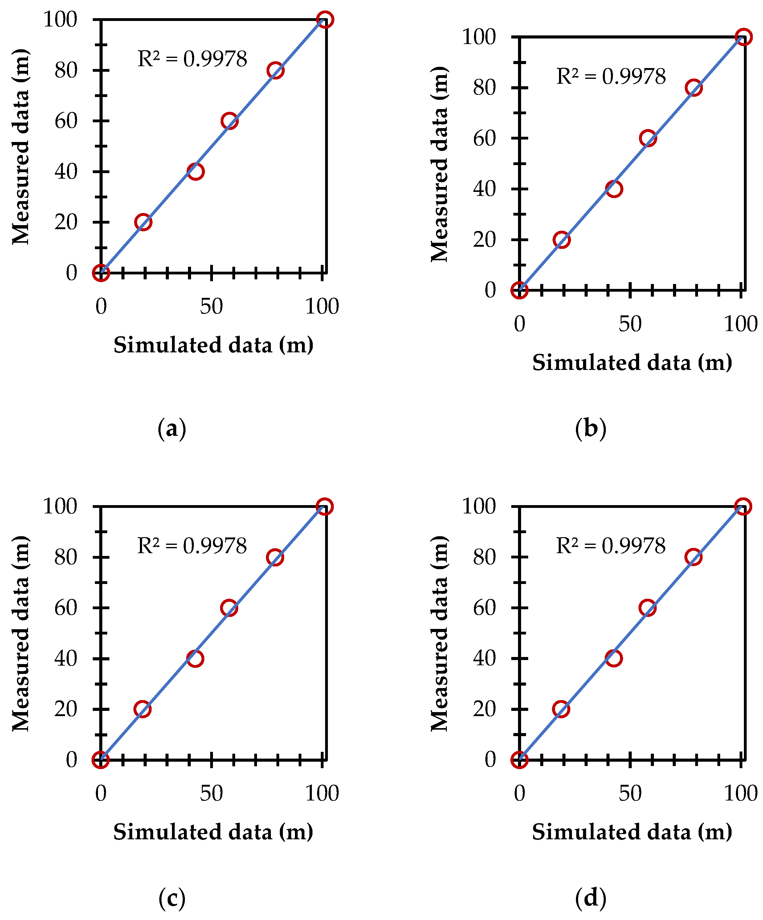
3.2. Numerical Validation

With the advance irrigation test data shown in Figure 4, the Levenberg–Marquardt linear optimization algorithm [32] was used to obtain the values of K_s = 1.54 cm/h and h_f = 38.00 cm. In the same figure, the good fit of the measured data of the advance phase and those obtained by the proposed model is observed, which yields an R² = 0.9978, so the proposed model adequately reproduces the data measured in the field.

Figure 5 shows the evolution of the water depth and infiltration at different points located along the border. It is observed that the subsurface flow follows the same tendency along the border, while the evolution of the water depth on the soil surface changes with the border position.

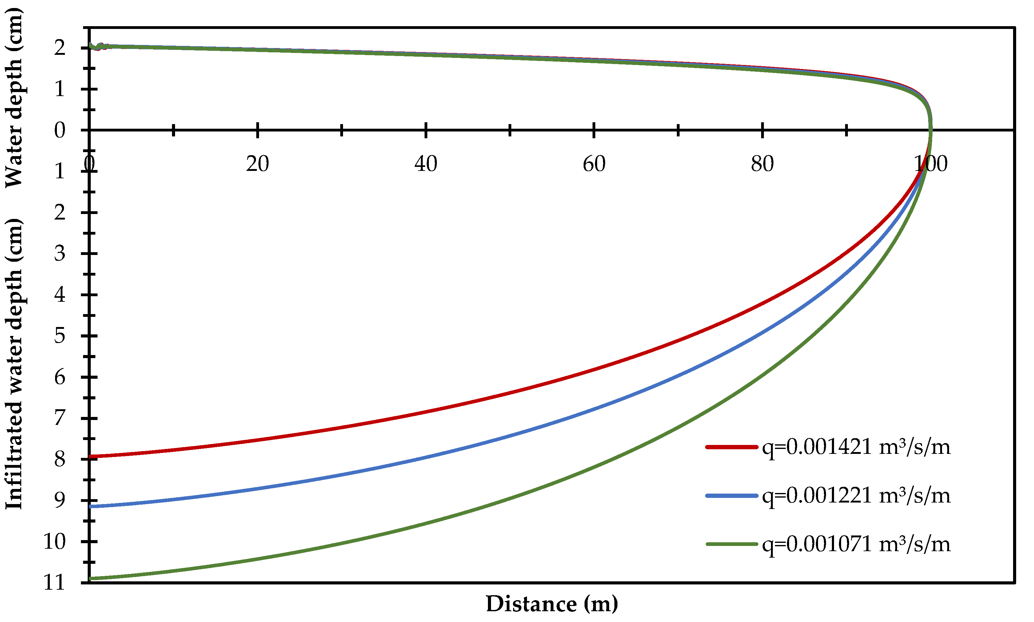
3.3. Comparison of Numerical Solutions

A comparison of the results of the advance irrigation test of the proposed model with the explicit model presented by Saucedo et al. [28] was made. In Figure 6, there are ideal adjustment for both models, however, it can be seen that, with the model developed here, the curve is adjusted better as the length of wave front increases, while the comparison model moves away to coincide exactly with the last point of the border. It is relevant to note that, to solve the coupling of the equations presented here, Saucedo et al. [28] used an explicit scheme (R² = 0.997) based on the coefficients proposed by Strelkoff and Katopodes [9], while in this work an implicit scheme (R² = 0.9978) was used.

The main advantage of the model presented here, which is implicit nature, is that all the computational cells of a given time are solved simultaneously, considering the current state of the flow profiles, as well as the next state, while the explicit model proposed by Saucedo et al. [28] only takes into account the current state of the flow profiles, which can generate problems to achieve the same accuracy at different δt.

With the optimized values of K_s and h_f from the irrigation test, the optimal irrigation flow was calculated, with Equation (16), using a net irrigation depth ${\ell }_{\mathrm{n}}$ = 10 cm and a border length L = 100 m, and a value of q_opt = 0.001221 m³/s/m was obtained. Figure 7 shows the infiltrated water depths and the variation in the flow rate at different times with 20 m of incremental advance.

The calculation of the optimal irrigation flow must be performed with extreme caution, since a different value may cause excess or deficit of water into the soil profile. Figure 8 shows how a variation by 1.5 l/s in the inlet flow can significantly modify the volume of infiltrated water, this is because with smaller flows the water at the surface has a lower velocity, which causes the contact time of the water with the soil to be longer and increases the infiltrated depth or volume of infiltrated water.

3.4. Efficient Computation

Having identified that one of the limitations of this model is the computation time required to obtain the solution (direct or inverse), we proceeded to perform the same simulations by increasing the time step; the results are shown in

Table 1. Computation time for different time steps δt.

δt (s)	Computer Time (min)	R2
1.0	4.70	0.9978
1.5	2.10	0.9978
2.0	1.16	0.9978
5.0	0.21	0.9978
10.0	0.06	0.9978

. The computer equipment used to perform the simulations has an Intel^® Core^TM i7-4710 CPU @ 2.50 GHz and 32 Gb of RAM.

Comparisons of the measured data and the results obtained with the proposed model can be seen in Figure 9.

4. Discussion

The computation time used to solve the inverse problem was 16 min and 4.70 min for the direct problem. Although the computation time required by Saucedo et al. [28] to simulate the direct problem is less (23 s) than the time required here, in the implicit scheme used here, all cells of a δt are solved at the same time, while for the explicit scheme, cell by cell is calculated. In addition, the results obtained reflect a lower error in the estimation of the parameters and simulation of the advance phase with respect to the data measured in the field, knowing that the scheme proposed here requires a higher computational cost.

To solve the direct or inverse problem by the explicit method in the same time step (δt = 1 s) requires more computational resources, however, it is compensated by having a higher accuracy in the simulated data with the measured data, which is reflected in a decrease in the error. Furthermore, the model proposed here has the advantage that, if we increase the δt to 10 s, the computation time decreases by 98.80% and the results of measured versus simulated data are excellent.

It is also seen that there is no difference for the different δt studied here, therefore, for design purposes, it is possible to use δt = 10 s to increase the processing speed and, thus, give a fast response to the advance/infiltration process in each irrigation plot. It is recommended to use, for research purposes, δt as close to the practical situation as possible, to observe the phenomenon closer to reality and produce solutions with high impact for society.

The model used here to calculate the hydrodynamic parameters of the soil, necessary to obtain the optimal irrigation flow through the solution of the inverse problem using the Levenberg–Marquardt optimization algorithm, showed excellent results. This water flow allows the application of a uniform irrigation depth, with zero water losses due to runoff and minimum losses due to deep infiltration (percolation).

According to the solution obtained, instability was observed in the first calculation cells by applying the n coefficient, where the higher the value of this coefficient, the instability, was considerably reduced until it disappeared on the drawing scale. The hydraulic resistance law used provides the facility to study and analyze irrigation tests in very large irrigation borders, which give us the option of using it for different flow regimes.

5. Conclusions

A numerical solution of the Barré de Saint-Venant equations coupled to the Green and Ampt equation was implemented to describe the advance phase of the border irrigation. The proposed solution of the model uses a Lagrangian finite differences scheme, which is solved from the Newton–Raphson method. Evaluation of the model in the simulation of the advance phase revealed that it fits well with field measurements.

Finally, the solution shown here can be used with excellent results to design and model border irrigation, as the infiltration equation used for a constant initial moisture profile uses characteristic soil parameters (K_s and h_f). This makes it a robust and efficient model compared to other models reported in the literature that use infiltration equations without a physical basis, such as Kostiakov and Kostiakov–Lewis. Additionally, it enables calculating the optimal irrigation flow to make water use efficiently in gravity irrigation systems.

References

1. Fuentes, C.; De León-Mojarro, B.; Hernández-Saucedo, F.R. Gravity irrigation hydraulics. In Gravity Irrigation; Fuentes, C., Rendón, L., Eds.; Nacional Association of Irrigation Specialist: Mexico, Spain, 2017; pp. 1–66. [Google Scholar]
2. Soroush, F.; Fenton, J.D.; Mostafazadeh-Fard, B.; Mousavi, S.F.; Abbasi, F. Simulation of furrow irrigation using the Slow-change/slow-flow equation. Agric. Water Manag. 2013, 116, 160–174. [Google Scholar] [CrossRef]
3. Akbari, M.; Gheysari, M.; Mostafazadeh-Fard, B.; Shayannejad, M. Surface irrigation simulation-optimization model based on meta-heuristic algorithms. Agric. Water Manag. 2018, 201, 46–57. [Google Scholar] [CrossRef]
4. Khasraghi, M.M.; Sefidkouhi, M.A.G.; Valipour, M. Simulation of Open- and Closed-End Border Irrigation Systems Using SIRMOD. Arch. Agron. Soil Sci. 2015, 61, 929–941. [Google Scholar] [CrossRef]
5. Chávez, C.; Fuentes, C. Design and evaluation of surface irrigation systems applying an analytical formula in the irrigation district 085, La Begoña, Mexico. Agric. Water Manag. 2019, 221, 279–285. [Google Scholar] [CrossRef]
6. Ebrahimian, H.; Liaghat, A. Field Evaluation of Various Mathematical Models for Furrow and Border Irrigation Systems. Soil Water Res. 2011, 6, 91–101. [Google Scholar] [CrossRef] [Green Version]
7. Sayari, S.; Rahimpour, M.; Zounemat-Kermani, M. Numerical Modeling Based on a Finite Element Method for Simulation of Flow in Furrow Irrigation. Paddy Water Environ. 2017, 15, 879–887. [Google Scholar] [CrossRef]
8. Singh, V.; Bhallamudi, S.M. Complete Hydrodynamic Border-Strip Irrigation Model. J. Irrig. Drain. Eng. 1996, 122, 189–197. [Google Scholar] [CrossRef]
9. Strelkoff, T.; Katopodes, N.D. Border-Irrigation Hydraulics with Zero Inertia. J. Irrig. Drain. Div. 1977, 103, 325–342. [Google Scholar]
10. Liu, K.H.; Jiao, X.Y.; Li, J.; An, Y.H.; Guo, W.H.; Salahou, M.K.; Sang, H. Performance of a Zero-Inertia Model for Irrigation with Rapidly Varied Inflow Discharges. Int. J. Agric. Biol. Eng. 2020, 13, 175–181. [Google Scholar] [CrossRef]
11. Bautista, E.; Schlegel, J.L.; Clemmens, A.J. The SRFR 5 Modeling System for Surface Irrigation. J. Irrig. Drain. Eng. 2016, 142, 04015038. [Google Scholar] [CrossRef]
12. Zhang, S.; Xu, D.; Bai, M.; Li, Y.; Liu, Q. Fully Hydrodynamic Coupled Simulation of Surface Flows in Irrigation Furrow Networks. J. Irrig. Drain. Eng. 2016, 142, 04016014. [Google Scholar] [CrossRef]
13. Brufau, P.; García-Navarro, P.; Playán, E.; Zapata, N. Numerical modeling of basin irrigation with an upwind scheme. J. Irrig. Drain. Eng. 2002, 128, 212–223. [Google Scholar] [CrossRef] [Green Version]
14. Gillies, M.H.; Smith, R.J. SISCO: Surface irrigation simulation, calibration and optimization. Irrig. Sci. 2015, 33, 339–355. [Google Scholar] [CrossRef]
15. Abbasi, F.; Shooshtari, M.M.; Feyen, J. Evaluation of various surface irrigation numerical simulation models. J. Irrig. Drain. Eng. 2003, 129, 208–213. [Google Scholar] [CrossRef]
16. Zerihun, D.; Furman, A.; Warrick, A.W.; Sanchez, C.A. Coupled surface-subsurface flow model for improved basin irrigation management. J. Irrig. Drain. Eng. 2005, 131, 111–128. [Google Scholar] [CrossRef]
17. Wöhling, T.; Fröhner, A.; Schmitz, G.H.; Liedl, R. Efficient Solution of the Coupled One-Dimensional Surface—Two-Dimensional Subsurface Flow during Furrow Irrigation Advance. J. Irrig. Drain. Eng. 2006, 132, 380–388. [Google Scholar] [CrossRef]
18. Tabuada, M.A.; Rego, Z.J.C.; Vachaud, G.; Pereira, L.S. Modelling of Furrow Irrigation. Advance with Two-Dimensional Infiltration. Agric. Water Manag. 1995, 28, 201–221. [Google Scholar] [CrossRef]
19. Woolhiser, D.A. Simulation of Unsteady Overland Flow. In Unsteady Flow in Open Channels; Water Resources Publications: Fort Collins, Colorado, 1975; Volume 2, pp. 485–508. [Google Scholar]
20. Banti, M.; Zissis, T.; Anastasiadou-Partheniou, E. Furrow Irrigation Advance Simulation Using a Surface–Subsurface Interaction Model. J. Irrig. Drain. Eng. 2011, 137, 304–314. [Google Scholar] [CrossRef]
21. Green, W.H.; Ampt, G.A. Studies on soil physics I: The flow of air and water through soils. J. Agric. Sci. 1911, 4, 1–24. [Google Scholar]
22. Zatarain, F.; Fuentes, C.; Rendón, L.; Vauclin, M. Effective soil hydrodynamic properties in border irrigation. Ing. Hidraul. Mexico 2003, 18, 5–15. [Google Scholar]
23. Fuentes, C.; Chávez, C. Analytic Representation of the Optimal Flow for Gravity Irrigation. Water 2020, 12, 2710. [Google Scholar] [CrossRef]
24. Elliott, R.L.; Walker, W.R.; Skogerboe, G.V. Zero-Inertia Modeling of Furrow Irrigation Advance. J. Irrig. Drain. Div. 1982, 108, 179–195. [Google Scholar]
25. Wallender, W.W.; Rayej, M. Shooting method for Saint Venant equations of furrow irrigation. J. Irrig. Drain. Eng. 1990, 116, 114–122. [Google Scholar] [CrossRef]
26. Liu, K.; Huang, G.; Xu, X.; Xiong, Y.; Huang, Q.; Šimůnek, J. A Coupled Model for Simulating Water Flow and Solute Transport in Furrow Irrigation. Agric. Water Manag. 2019, 213, 792–802. [Google Scholar] [CrossRef] [Green Version]
27. Liu, K.; Xiong, Y.; Xu, X.; Huang, Q.; Huo, Z.; Huang, G. Modified Model for Simulating Water Flow in Furrow Irrigation. J. Irrig. Drain. Eng. 2020, 146, 06020002. [Google Scholar] [CrossRef]
28. Saucedo, H.; Zavala, M.; Fuentes, C. Use of Saint-Venant and Green and Ampt equations to estimate infiltration parameters based on measurements of the water front advance in border irrigation. Water Technol. Sci. 2016, 7, 117–124. [Google Scholar]
29. Walker, W.R.; Skogerboe, G.V. Surface Irrigation. Theory and Practice; Prentice-Hall, Inc.: Englewood Cliffs, NJ, USA, 1987. [Google Scholar]
30. Strelkoff, T. EQSWP: Extended unsteady-flow double-sweep equation solver. J. Hydraul. Eng. 1992, 118, 735–742. [Google Scholar]
31. USDA-NRCS. National Engineering Handbook, Part 652. In Irrigation Guide—USDA: Natural Resources Conservation Service; USDA-NRCS: Washington, DC, USA, 1997; p. 754. [Google Scholar]
32. Moré, J.J. The Levenberg-Marquardt algorithm: Implementation and theory. In Numerical Analysis; Springer: Berlin/Heidelberg, Germany, 1978; pp. 105–116. [Google Scholar]
Figure 1. Typical border irrigation scheme.
Mathematics 10 01039 g001
Figure 2. Computational grid for the advance phase.
Mathematics 10 01039 g002
Figure 3. Water depth/infiltration curves for different Manning n values.
Mathematics 10 01039 g003
Figure 4. Advance curve of the measured data and those obtained with the optimization of the parameters.
Mathematics 10 01039 g004
Figure 5. Evolution of the water depth and infiltration in different points of the border.
Mathematics 10 01039 g005
Figure 6. Comparison between the data measured, those simulated by the model with optimized parameters and those reported in the ref. [28].
Mathematics 10 01039 g006
Figure 7. Advance curves and infiltrated water with 20 m of incremental advance.
Mathematics 10 01039 g007
Figure 8. Advance curves with different unitary discharge in the border.
Mathematics 10 01039 g008
Figure 9. Relation between the data measured and those simulated by the model with parameters optimized at different time steps (δt). (a) δt = 1.5 s; (b) δt = 2.0 s; (c) δt = 5.0 s; (d) δt = 10.0 s.
Mathematics 10 01039 g009