A Modified Power Family of Distributions: Properties, Simulations and Applications

Abstract

In this paper, we present a new class of distributions called the modified power family by adding an extra shape parameter. Some of its structural properties are derived. Three special cases of the new family are considered and estimated using the method of maximum likelihood. The validity of the method of maximum likelihood is illustrated via Monte Carlo simulations. The importance and flexibility of the new family are empirically illustrated, partly due to efficient modeling of several real data. We compare the proposed family with some distributions and special models generated from other classes using classical statistical measures.

1. Introduction

Several papers introduced, in the last three decades, new classes of continuous distributions with desirable properties and motivations from a baseline cumulative distribution function (cdf) $G\left(x\right)$. Ref. [1] proposed the Marshall–Olkin-G family, with applications to the exponential and Weibull distributions, using an extra shape parameter to make more flexible the generated distributions. Based on the Marshall–Olkin-G family, several models were investigated: Marshall–Olkin–Weibull [2], Marshall–Olkin–Lomax [3], Marshal–Olkin–Fréchet [4], Marshall– Olkin Burr XII  [5] and modified-power-function [6] distributions, among others.

Another method to generate a new cdf [7] is the beta-G family by composing the cdf of the beta distribution with $G\left(x\right)$, i.e., $F\left(x\right)=I_{G\left(x\right)}(a,b)$, where $I_x(a,b)$ is the incomplete beta function ratio. Several articles were published on sub-models of the beta-G family such as the beta-exponential [8], beta-generalized-exponential [9] and beta-Dagum [10], among several others.

This composition procedure was extended to a function of $G\left(x\right)$ ($W\left[G\right(x\left)\right]$), instead of $G\left(x\right)$, in [11,12,13,14], to generate the gamma-G, Kumaraswamy-G, gamma-G and log-gamma-G (I and II). For more details about composition of cdfs, see, for example, [15,16,17].

Recently, Refs. [18,19] followed the same proposal by [1], and starting with a monotone increasing function of $G\left(x\right)$, defined the alpha-power-G classes with cdfs including one and two extra parameters, respectively, given by

$$F_{AP}\left(x\right)=\frac{{\alpha }^{G\left(x\right)}-1}{\alpha -1},\mathrm{for}\alpha >0,\alpha \ne 1,$$

$$F_{MAP}\left(x\right)=\frac{{\alpha }^{G^2\left(x\right)}{\beta }^{G\left(x\right)}-1}{\alpha \beta -1},\mathrm{for}\alpha ,\beta \ge 1,\alpha \beta \ne 1.$$

In this paper, we present a new family with one extra parameter based on the parent cdf $G\left(x\right)$. Our aim is to show its utility to achieve adequate flexibility to real data in many fields. The new family is motivated by the ability to fit real data. The cdf and probability density function (pdf) of the new family have simple expressions. The density shapes can be decreasing or unimodal (right-skewed or symmetrical). The hazard rate function (hrf) exhibits monotone, non-monotone (bathtub and upside-down bathtub) or decreasing–increasing–decreasing shapes.

The rest of the paper is structured as follows. Section 2 defines a new one-parameter family, provides some of its properties and discusses the estimation method. Three sub-models are addressed in Section 3. Section 4 examines the efficiency of the estimators via Monte Carlo simulations, and performs real applications of these sub-models. Finally, Section 5 concludes the paper.

2. Materials and Methods

2.1. The New Family

Definition 1.

For every continuous cdf $G\left(x\right)$, the cdf of the modified power (MPo) family is defined by the monotonic increasing cdf $F:\mathbb{R}\to [0,1]$ (for $x\in \mathbb{R}$)

$$F\left(x\right)=a^{G\left(x\right)-1}G\left(x\right),\mathrm{if}a\ge {\mathrm{e}}^{-1}.$$

(1)

It is clear that ${lim}_{x\to -\infty }F\left(x\right)=0$ and ${lim}_{x\to \infty }F\left(x\right)=1$. For $a=1$, $F\left(x\right)=G\left(x\right)$.

The pdf corresponding to (1) is

$$f\left(x\right)=a^{G\left(x\right)-1}g\left(x\right)\left[1+G\left(x\right)lna\right],$$

(2)

where $g\left(x\right)=dG\left(x\right)/dx$ is the baseline density corresponding to $G\left(x\right)$.

Proposition 1.

Equation (2) is a weighted function of the baseline density $g\left(x\right)$, where

$$w\left(x\right)=a^{G\left(x\right)}\left[1+G\left(x\right)lna\right]$$

is the weight. Note that $w\left(x\right)$ is increasing for $a>1$, and decreasing for $a<1$. Equation (2) leads to

$$f\left(x\right)=\frac{1}{a}w\left(x\right)g\left(x\right).$$

(3)

For the parent random variable (rv) $T\sim G$ by integrating both sides of (3) gives $E\left[w\left(T\right)\right]=a$.

These weights play an important role in distribution theory [20]. The weighted distributions are very important, because they consider the method of ascertainment by adjusting the probabilities of actual occurrence of events. Ref. [21] introduced the concept of a weighted distribution as a method of adjustment applicable to many situations. We may arrive at the wrong conclusions, while failing to make such an adjustment.

Many authors have employed weighted distributions for different purposes, see [22,23]. They occur frequently in reliability, meta analysis and analysis of intervention data, biomedicine and several other areas, for the improvement of proper statistical models.

We denote the hrfs corresponding to F and G by $h_F\left(x\right)$ and $h_G\left(x\right)$, respectively. From Equation (3), the following results compare some measures of the weighted rv $X\sim F$ with those of the unweighted $T\sim G$ [24]:

(i)

If $w\left(x\right)$ is monotone increasing $h_F\left(x\right)\le h_G\left(x\right)$ and then $F\left(x\right)\le G\left(x\right)$ for all x.

(ii)

If $w\left(x\right)$ is monotone decreasing, $h_G\left(x\right)\le h_F\left(x\right)$ and then $G\left(x\right)\le F\left(x\right)$ for all x.

(iii)

$E\left(X\right)>E\left(T\right)$ if $Cov(T,w(T\left)\right)>0$.

(iv)

$E\left(X\right)<E\left(T\right)$ if $Cov(T,w(T\left)\right)<0$.

Properties (i) and (ii) are illustrated in Figure 1 for the exponential baseline distribution. For two monotone increasing weights $w(x;2,5)$ and $w(x;3,5)$ and two monotone decreasing weights $w(x;0.5,5)$ and $w(x;0.6,5)$.

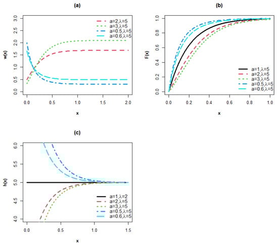
Figure 1. Plots of the (a) weight, (b) cdf and (c) hrf for the MPoE model.

Several others interesting connections between measures of X and T in the context of reliability and life testing were addressed by [22].

The cdf of the “exponentiated-G” (exp-G) class is simply given by ${\Pi }_b\left(x\right)=G{\left(x\right)}^b$, where $G\left(x\right)$ is the baseline cdf and $b>0$ is a power parameter. So, the pdf of the exp-G class is ${\pi }_b\left(x\right)=bG{\left(x\right)}^{b-1}g\left(x\right)$, where $g\left(x\right)$ is the parent pdf. Twenty eight different exp-G models were reported in Table 1 of [16] with a complete and accurate bibliography until this date.

Proposition 2.

The density of X is an infinite linear combination of exponentiated densities with weights $p_i={(lna)}^i/(i!a)(\mathrm{for}\mathrm{i}=0,1,\dots )$

Proof. 

Using the power series for $a^{G\left(x\right)}$, Equation (1) reduces to

$$F\left(x\right)=\frac{1}{a}\sum _{i=0}^{\infty }\frac{{\left(lna\right)}^i}{i!}G{\left(x\right)}^{i+1},$$

and the density of X can be written as

$$f\left(x\right)=\frac{1}{a}\sum _{i=0}^{\infty }\frac{{\left(lna\right)}^i}{i!}{\pi }_{i+1}\left(x\right),$$

(4)

where ${\pi }_{i+1}\left(x\right)=(i+1)g\left(x\right)G{\left(x\right)}^i$ is the exp-G density with power $i+1$.    □

Hence, based on the linear representation (4), some properties of the new family follow from those exp-G properties reported in several papers; see Table 1 of [16]. Henceforth, $Y_{i+1}$ denotes a rv with density ${\pi }_{i+1}\left(x\right)$.

2.2. Moments

If X has density (2), the rth ordinary moment of X (for $r=1,2,\dots$) can be found from (4) and the moments of the exp-G distribution as

$${\mu }_r^{\prime }=E\left(X^r\right)=\frac{1}{a}\sum _{i=0}^{\infty }\frac{{\left(lna\right)}^i}{i!}E\left(Y_{i+1}^r\right)=\frac{1}{a}{\int }_0^1{a}^y{\left[G^{-1}\left(y\right)\right]}^r\left[1+ylna\right]dy.$$

The rth incomplete moment of X comes from (4)

$$I_X\left(t;r\right)=E\left(X^r\mid X\le t\right)=\frac{1}{a}\sum _{i=0}^{\infty }\frac{{\left(lna\right)}^i}{i!}{\int }_{-\infty }^t{x}^r{\pi }_{i+1}\left(x\right)dx=\frac{1}{a}\sum _{i=0}^{\infty }\frac{{\left(lna\right)}^i}{i!}{I}_i\left(t;r\right),$$

where $I_i\left(t;r\right)$ is the rth incomplete moment of $Y_{i+1}$.

The first incomplete moment $I_X\left(t;1\right)$ is useful for determining the mean deviations from any location of X, and the Bonferroni and Lorenz curves.

2.3. Generating Function

The generating function (gf) of X can be found from (4)

$$M_X\left(t\right)=\frac{1}{a}\sum _{i=0}^{\infty }\frac{{\left(lna\right)}^i}{i!}{M}_i\left(t;r\right),$$

where $M_i\left(t\right)$ is the gf of $Y_{i+1}$ Alternatively, the gf of X can be written as

$$M_X\left(t\right)=\frac{1}{a}{\int }_0^1{a}^{y}exp\left[t{G}^{-1}\left(y\right)\right]\left[1+ylna\right]dy.$$

By expanding $a^y$ in power series gives

$$M_X\left(t\right)=\frac{1}{a}\sum _{i=0}^{\infty }\frac{{\left(lna\right)}^i}{i!}{\int }_0^1{y}^{i}exp\left[t{G}^{-1}\left(y\right)\right]\left[1+ylna\right]dy.$$

2.4. Quantiles

There is no explicit form for the quantile function (qf) of X, but it can be approximated using a one-dimensional root-finding algorithm from (1) such as Newton’s method in $F\left(z\right)-u=z{a}^{z-1}-u=0$, where $G\left(x\right)=z$. We can write the iterative process as

$$z_{i+1}=z_i-\frac{z_i-u{a}^{1-z_i}}{(1+z_{i}loga)}$$

and starting with a suitable guess and keep repeating the process (for $i\ge 1$) until terminate at $z^{\star }$ for a specified accuracy level. So, we obtain $x=G^{-1}\left(z^{\star }\right)$. Further, the solution of z in $F\left(z\right)=z{a}^{z-1}=u$ is given by (Using the Mathematica software)

$$z=W_0\left(aulna\right)/lna,\mathrm{for}a\ne 1,$$

where $W_0$ is the principal branch of the Lambert W function, which has a known power series

$$z=W_0\left(u\right)=\sum _{i=1}^{\infty }\frac{{(-1)}^{i+1}{i}^{i-2}}{(i-1)!}{u}^i.$$

So, the qf of X follows from the baseline qf as

$$x=Q\left(u\right)=G^{-1}\left(W_0\left(aulna\right)/lna\right),\mathrm{for}a\ne 1.$$

2.5. Mode

The mode m of the MPo family can be found by maximizing the log-pdf from (2). At $x=m$, the derivative of $lnf\left(x\right)$ with respect to x vanishes. We can obtain m by solving the equation

$$\frac{g^{\prime }\left(m\right)}{g\left(m\right)}+g\left(m\right)lna+\frac{g\left(m\right)lna}{1+G\left(m\right)lna}=0,$$

(5)

which has no explicit solution for m. So, the mode of the MPo family does not have a closed form. Given $F(·)$ and $f(·)$, direct maximization of $lng\left(x\right)$ using a numerical optimization algorithm or one-dimensional root-finding algorithm of (5) can be used to approximate the mode.

2.6. Hazard Rate

The hrf of X is

$$\begin{array}{c}\hfill h_F\left(x\right)=\frac{a^{G\left(x\right)}[1+G\left(x\right)lna][1-G\left(x\right)]}{a-a^{G\left(x\right)}G\left(x\right)}{h}_G\left(x\right).\end{array}$$

Proposition 3.

It is straightforward to show that:

$$\underset{x\to -\infty }{lim}{h}_F\left(x\right)=\frac{1}{a}\underset{x\to -\infty }{lim}{h}_G\left(x\right),\underset{x\to \infty }{lim}{h}_F\left(x\right)=\underset{x\to \infty }{lim}{h}_G\left(x\right).$$

2.7. Estimation

Let $x_1,\dots ,x_n$ be n independent realizations from the MPo model, ${\eta }^{\top }=(a,{\theta }^{\top })$, where $\theta$ is the parameter vector of the parent distribution. The log-likelihood function for $\eta$ is

$$\ell \left(\eta \right)=-nlna+lna\sum _{i=1}^{n}G\left(x_i;\theta \right)+\sum _{i=1}^{n}lng\left(x_i;\theta \right)+\sum _{i=1}^{n}ln\left[1+G\left(x_i;\theta \right)lna\right].$$

By differentiating $\ell \left(\eta \right)$ with respect to the parameters, we obtain the score components:

$$U_a=-\frac{n}{a}+\frac{1}{a}\sum _{i=1}^{n}G\left(x_i;\theta \right)+\frac{1}{a}\sum _{i=1}^n\frac{G\left(x_i;\theta \right)}{1+G\left(x_i;\theta \right)lna}$$

and

$$U_{\theta }=lna\sum _{i=1}^n\frac{\partial G\left(x_i;\theta \right)}{\partial \theta }+\sum _{i=1}^n\frac{1}{g\left(x_i;\theta \right)}\frac{\partial g\left(x_i;\theta \right)}{\partial \theta }+\sum _{i=1}^n\frac{lna}{1+G\left(x_i;\theta \right)lna}\frac{\partial G\left(x_i;\theta \right)}{\partial \theta }.$$

Since we can not solve these equations analytically to find the maximum likelihood estimates (MLEs) of $(a,\theta )$, these estimates $(\widehat{a},\widehat{\theta })$ can be determined by numerical algorithms, such as the BFGS algorithm. This algorithm with analytical derivatives can be used for maximizing $\ell \left(\eta \right)$ using the R software library AdequacyModel [25], which provides a general optimization method for maximizing or minimizing an arbitrary objective function.

3. Sub-Models

3.1. Modified Power Exponential (MPoE)

For the exponential parent with rate $\lambda >0$, the cdf of the MPoE model (for $x>0$ and $a\ge {\mathrm{e}}^{-1}$) is

$$\begin{array}{c}\hfill F\left(x\right)=a^{-exp\left(-\lambda x\right)}\left[1-exp\left(-\lambda x\right)\right].\end{array}$$

Plots of the pdf, cdf and hrf of the MPoE are displayed in Figure 2.

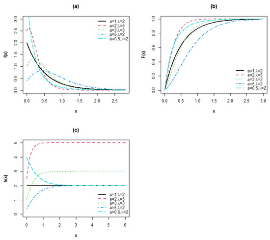
Figure 2. Plots of the (a) pdf, (b) cdf and (c) hrf for the MPoE model.

3.2. Modified Power Weibull (MPoW)

For the Weibull with shape $k>0$ and scale $\lambda >0$, the cdf of the MPoW model (for $x>0$ and $a\ge {\mathrm{e}}^{-1}$) is

$$\begin{array}{c}\hfill F\left(x\right)=a^{-exp\left[-{\left(x/\lambda \right)}^k\right]}\left\{1-exp\left[-{\left(x/\lambda \right)}^k\right]\right\}.\end{array}$$

Plots of the pdf, cdf and hrf of the MPoW are reported in Figure 3.

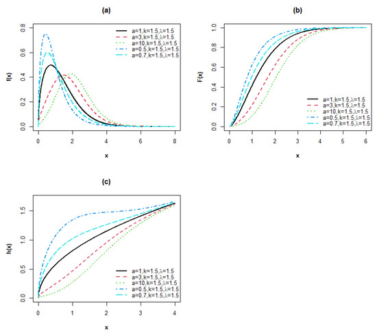
Figure 3. Plots of the (a) pdf, (b) cdf and (c) hrf for the MPoW model.

3.3. Modified Power Fréchet (MPoF)

For the Fréchet with shape $k>0$ and scale $\lambda >0$, the cdf of the MPoF model (for $x>0$ and $a\ge {\mathrm{e}}^{-1}$) is

$$\begin{array}{c}\hfill F\left(x\right)=a^{exp\left[\left(-{(x/\lambda )}^{-k}\right)\right]-1}exp\left[-{(x/\lambda )}^{-k}\right].\end{array}$$

Plots of the pdf, cdf and hrf of the MPoF are displayed in Figure 4.

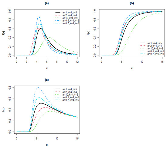
Figure 4. Plots of the (a) pdf, (b) cdf and (c) hrf for the MPoF model.

4. Applications

4.1. Simulation Results

A simulation was conducted to examine the accuracy of the MLEs for the MPoE and MPoW distributions. Their averages, absolute biases (ABs) and mean square errors (MSEs) are calculated from 1000 samples of sizes n = 50, 100, 150 and 250 with different values of parameters. Table 1 and Table 2 provide the results. The MLEs and ABs in Table 1 and Table 2 indicate that the ML method provides parameter estimates, which converge to the true parameter values and the MSEs decrease when n increases. These results reflect the appropriateness of the ML method to provide good estimates of the parameters of the MPo distribution.

Table 1. Simulation results for the MPoE distribution.

Parameters				$\widehat{\mathit{a}}$			$\widehat{\mathit{\lambda }}$
$\mathit{\lambda }$	$\mathit{a}$	$\mathit{n}$	Average	AB	MSE	Average	AB	MSE
0.5	0.7	50	0.882822	0.182822	0.240279	0.550483	0.050483	0.032359
		100	0.773099	0.073099	0.085056	0.512771	0.012772	0.017368
		150	0.748480	0.048480	0.055557	0.506860	0.006860	0.013133
		250	0.722869	0.022869	0.034346	0.498502	0.001498	0.009568
	1.5	50	1.965970	0.465970	2.054128	0.520573	0.020573	0.013476
		100	1.671669	0.171669	0.446837	0.505050	0.005050	0.006096
		150	1.623362	0.123362	0.278527	0.505484	0.005484	0.003993
		250	1.570789	0.070789	0.154100	0.501920	0.001920	0.002371
	2	50	2.712318	0.712318	5.774216	0.517803	0.017803	0.011185
		100	2.263772	0.263772	0.971162	0.507723	0.007723	0.005344
		150	2.194257	0.194257	0.608456	0.505588	0.005588	0.003508
		250	2.111141	0.111141	0.294932	0.503429	0.003429	0.002035
	3	50	4.075306	1.075306	13.50904	0.509365	0.009365	0.008007
		100	3.496485	0.496485	3.626017	0.504492	0.004492	0.003910
		150	3.295536	0.295536	1.733014	0.500741	0.000741	0.003283
		250	3.181315	0.181315	0.782124	0.501969	0.001969	0.001510
2	0.7	50	0.943534	0.243534	0.384633	2.278365	0.278365	0.570959
		100	0.805673	0.105673	0.101692	2.125072	0.125072	0.310716
		150	0.761194	0.061194	0.061672	2.058762	0.058762	0.227969
		250	0.736927	0.036927	0.035083	2.028866	0.028866	0.152910
	1.5	50	1.900829	0.400829	1.863967	2.053579	0.053579	0.209653
		100	1.648641	0.148641	0.426688	2.024280	0.024280	0.097089
		150	1.613782	0.113782	0.258661	2.015773	0.015773	0.064948
		250	1.558614	0.058614	0.134646	2.006489	0.006489	0.036532
	2	50	2.684016	0.684016	3.802964	2.064413	0.064413	0.164225
		100	2.278580	0.278580	1.083252	2.029290	0.029290	0.086217
		150	2.190362	0.190362	0.573666	2.024598	0.024598	0.056450
		250	2.107925	0.107925	0.293745	2.015824	0.015824	0.032229
	3	50	4.377960	1.377960	31.40547	2.049894	0.049894	0.124898
		100	3.512797	0.512797	3.638915	2.018665	0.018665	0.060938
		150	3.303617	0.303617	1.592218	2.016532	0.016532	0.040930
		250	3.151232	0.151232	0.793243	2.007276	0.007276	0.024177
3	0.7	50	0.873411	0.173411	0.249293	3.257954	0.257954	1.066165
		100	0.786636	0.086636	0.098061	3.135110	0.135110	0.665893
		150	0.748945	0.048945	0.056103	3.060700	0.060700	0.512111
		250	0.721372	0.021372	0.034545	2.996890	0.003102	0.367859
	1.5	50	1.954494	0.454494	1.887515	3.110148	0.110148	0.530597
		100	1.649660	0.149660	0.440642	3.038955	0.038955	0.227560
		150	1.593534	0.093534	0.242919	3.024420	0.024420	0.138723
		250	1.543260	0.043260	0.123777	3.010334	0.010334	0.079245
	2	50	2.672203	0.672203	7.185814	3.099685	0.099685	0.401843
		100	2.255006	0.255006	1.004361	3.043369	0.043369	0.173005
		150	2.146790	0.146790	0.513999	3.023442	0.023442	0.113553
		250	2.091436	0.091436	0.283326	3.012997	0.012997	0.067657
	3	50	4.379168	1.379168	20.19350	3.089807	0.089807	0.304051
		100	3.440796	0.440796	2.437569	3.039237	0.039237	0.126145
		150	3.291080	0.291080	1.489429	3.022131	0.022131	0.085193
		250	3.141794	0.141794	0.713955	3.007916	0.007916	0.052587

Table 2. Simulation results for the MPoW distribution.

Parameters						$\widehat{\mathit{a}}$			$\widehat{\mathit{k}}$			$\widehat{\mathit{\lambda }}$
$\mathit{\lambda }$	$\mathit{a}$	$\mathit{k}$	$\mathbf{n}$	Average	AB	MSE	Average	AB	MSE	Average	AB	MSE
2	0.5	0.7	50	0.6974	0.1974	0.1892	0.6043	0.0957	0.0177	1.2773	0.7227	0.0427
			100	0.4217	0.0783	0.1395	0.7591	0.0591	0.0151	1.5491	0.4509	0.0311
			150	0.5641	0.0641	0.1258	0.7409	0.0409	0.0144	1.5449	0.4551	0.0217
			250	0.5326	0.0326	0.0122	0.7082	0.0082	0.0104	2.1064	0.1064	0.0195
		1.5	50	0.6857	0.1857	0.4249	1.7212	0.2212	0.5996	1.5249	0.4751	0.0549
			100	0.6186	0.1186	0.2484	1.6268	0.1268	0.1522	2.2185	0.2185	0.0360
			150	0.5529	0.0529	0.2051	1.5904	0.0904	0.1432	2.2113	0.2113	0.0329
			250	0.4920	0.0080	0.0794	1.5378	0.0378	0.1389	2.0980	0.0980	0.0092
		2	50	0.3525	0.1475	0.2615	1.5593	0.4407	0.9883	1.2957	0.7043	0.0675
			100	0.5897	0.0897	0.1323	1.8908	0.1092	0.9417	2.6692	0.6692	0.0362
			150	0.5226	0.0226	0.0988	1.8959	0.1041	0.1018	2.3325	0.3325	0.0312
			250	0.4865	0.0135	0.0115	2.0077	0.0077	0.0176	1.9845	0.0155	0.0088
		3	50	0.6329	0.1329	0.1444	2.1296	0.8704	1.0534	1.7722	0.2278	0.0260
			100	0.4269	0.0731	0.0943	2.4227	0.5773	1.0384	1.8767	0.1233	0.0255
			150	0.5107	0.0107	0.0458	3.1738	0.1738	0.5766	1.8911	0.1089	0.0176
			250	0.5004	0.0004	0.0134	2.9105	0.0895	0.2378	2.0101	0.0101	0.0143
2	2	0.7	50	1.7145	0.2855	0.4656	0.8224	0.1224	0.9181	2.3900	0.3900	0.0180
			100	1.8528	0.1472	0.4017	0.6054	0.0946	0.1661	2.2525	0.2525	0.0174
			150	2.1760	0.1760	0.1472	0.7909	0.0909	0.0243	2.1926	0.1926	0.0144
			250	2.0068	0.0068	0.0324	0.7531	0.0531	0.0036	2.0848	0.0848	0.0032
		1.5	50	1.7044	0.2956	0.0463	1.0471	0.4529	0.0737	1.2915	0.7085	0.0437
			100	1.8400	0.1600	0.0403	1.1489	0.3511	0.0682	1.5404	0.4596	0.0217
			150	1.9327	0.0673	0.0388	1.6481	0.1481	0.0677	2.4543	0.4543	0.0217
			250	1.9996	0.0004	0.0355	1.6223	0.1223	0.0577	1.8594	0.1406	0.0197
		2	50	2.9023	0.9023	0.2937	1.4529	0.5471	0.4083	1.3418	0.6582	0.0476
			100	2.2017	0.2017	0.2610	2.0999	0.0999	0.3925	1.5995	0.4005	0.0432
			150	2.0383	0.0383	0.2424	1.9474	0.0526	0.2582	1.8849	0.1151	0.0371
			250	2.0109	0.0109	0.0635	1.9976	0.0024	0.004	1.9892	0.0108	0.0023
		3	50	1.9690	0.0310	0.6949	2.4170	0.5830	0.5339	2.2962	0.2962	0.1006
			100	2.0276	0.0276	0.1471	2.7471	0.2529	0.3515	2.2652	0.2652	0.0262
			150	1.9997	0.0003	0.1285	2.7598	0.2402	0.0444	1.8496	0.1504	0.0127
			250	2.0002	0.0002	0.0501	2.8914	0.1086	0.0188	1.9956	0.0044	0.0084
2	3	0.7	50	2.5618	0.4382	0.4656	0.8982	0.1982	0.9181	2.3644	0.3644	0.0180
			100	2.7620	0.2380	0.4017	0.8619	0.1619	0.1661	1.7083	0.2917	0.0174
			150	2.9340	0.0660	0.1472	0.5604	0.1396	0.0243	1.7568	0.2432	0.0144
			250	2.9765	0.0235	0.0324	0.8248	0.1248	0.0036	2.1115	0.1115	0.0032
		1.5	50	3.4140	0.4140	0.0463	1.0156	0.4844	0.0737	2.1701	0.1701	0.0437
			100	3.2584	0.2584	0.0403	1.2049	0.2951	0.0682	1.8485	0.1515	0.0217
			150	3.1511	0.1511	0.0388	1.4688	0.0312	0.0677	1.8622	0.1378	0.0217
			250	3.0254	0.0254	0.0355	1.4998	0.0002	0.0577	2.1085	0.1085	0.0197
		2	50	2.1690	0.8310	0.2937	2.9358	0.9358	0.4083	1.4333	0.5667	0.0476
			100	2.8785	0.1215	0.2610	2.3803	0.3803	0.3925	1.4732	0.5268	0.0432
			150	2.9671	0.0329	0.2424	2.3739	0.3739	0.2582	2.3819	0.3819	0.0371
			250	2.9907	0.0093	0.0635	2.3256	0.3256	0.004	1.9900	0.0100	0.0226
		3	50	2.4566	0.5434	0.6949	2.5022	0.4978	0.5339	2.3716	0.3716	0.1006
			100	2.4677	0.5323	0.1471	2.5756	0.4244	0.3515	2.1580	0.1580	0.0262
			150	2.6199	0.3801	0.1285	3.1543	0.1543	0.0444	2.1364	0.1364	0.0127
			250	3.0610	0.0610	0.0501	3.0506	0.0506	0.0188	1.9498	0.0502	0.0084

4.2. Real Data

4.2.1. Breast Cancer Data

We fit the sub-models defined in Section 3 to the data sets available in the UC Irvine Machine Learning Repository at the Diagnostic Wisconsin Breast Cancer Data [26]. The data contain 30 features (V3, V4, ..., V32). The MPoE model is adopted for fitting to V19, V20, V28 and V29. The MPoW model is used for fitting to V7, V11, V14, V18, V24 and V27. The MPoF model is chosen for fitting to V3, V5, V13 and V21.

Table 3, Table 4 and Table 5 report the MLEs and 95% confidence intervals (CIs) of the parameters. To test whether the data sets are drawn from these sub-models, Cramér–von Mises (CvM) and Kolmogorov–Smirnov (KS) statistics and their p-values are given in Table 6, Table 7 and Table 8. These findings prove that the hypothesis that the data come from the MPo distribution (with the corresponding estimates given in Table 3, Table 4 and Table 5) can not be rejected and then the three sub-models are good choices for modeling these data.

Table 3. MLEs and 95% CIs of the MPoE parameters.

Feature	MLEs		95% CI
	$\widehat{\mathit{a}}$	$\widehat{\mathit{\lambda }}$	$\widehat{\mathit{a}}$	$\widehat{\mathit{\lambda }}$
V19	3.9919	49.438	(2.2880,5.6959)	( 46.394,52.483)
V20	94.236	193.55	(82.612,105.86)	(188.48,198.62)
V28	45.628	8.6588	(37.896,53.361)	(7.5277,9.7900)
V29	2.8132	5.2714	(1.4788,4.1475)	(4.2615,6.2813)

Table 4. MLEs and 95% CIs of the MPoW parameters.

Feature	MLEs			95% CI
	$\widehat{\mathit{a}}$	$\widehat{\mathit{k}}$	$\widehat{\mathit{\lambda }}$	$\widehat{\mathit{a}}$	$\widehat{\mathit{k}}$	$\widehat{\mathit{\lambda }}$
V7	513.0912	3.3737	0.0745	(480.53,545.65)	(2.6428,4.1046)	(−0.0011,0.1502)
V11	702.6257	3.2001	0.1372	(666.79,738.46)	(2.5228,3.8775)	(0.0387,0.2356)
V14	408.6297	1.1562	0.5475	(380.58,436.66)	(0.7323,1.5800)	(0.2023,0.8927)
V18	522.4037	0.7512	0.0068	(491.36,553.44)	(0.4240,1.0785)	(−0.0379,0.0515)
V24	419.4847	2.0796	16.855	(387.74,451.23)	(1.4689,2.6903)	(15.288,18.423)
V27	291.9343	2.9491	0.0997	(267.52,316.35)	(2.2446,3.6535)	(0.0029,0.1965)

Table 5. MLEs and 95% CIs of the MPoF parameters.

Feature	MLEs			95% CI
	$\widehat{\mathit{a}}$	$\widehat{\mathbf{k}}$	$\widehat{\mathit{\lambda }}$	$\widehat{\mathit{a}}$	$\widehat{\mathit{k}}$	$\widehat{\mathit{\lambda }}$
V3	17.715	5.3628	9.8237	(10.229,25.201)	(4.5433,6.1823)	(8.5244,11.123)
V5	20.044	5.0960	62.197	(11.959,28.129)	(4.2956,5.8970)	(58.835,65.559)
V13	3.2160	2.4583	0.2096	(0.3508,6.0813)	(1.8403,3.0762)	(−0.0916,0.5107)
V21	9.8563	3.9452	0.0127	(2.4746,17.238)	(3.2336,4.6568)	(−0.0640,0.0894)

Table 6. Kolmogorov–Smirnov and Cramér–von Mises tests for the MPoE model.

Feature	CvM		KS
	Statistic	p-Value	Statistic	p-Value
V19	0.2460	0.1936	0.0375	0.4020
V20	0.3240	0.1158	0.0414	0.2847
V28	0.2366	0.2065	0.0442	0.2155
V29	0.0701	0.7513	0.0311	0.6401

Table 7. Kolmogorov–Smirnov and Cramér–von Mises tests for the MPoW model.

Feature	CvM		KS
	Statistic	p-Value	Statistic	p-Value
V7	0.0838	0.6706	0.0306	0.6510
V11	0.2296	0.2168	0.0393	0.3418
V14	0.0906	0.6332	0.0352	0.4819
V18	0.2055	0.2571	0.0408	0.3000
V24	0.0694	0.7555	0.0295	0.7052
V27	0.0477	0.8904	0.0248	0.8738

Table 8. Kolmogorov–Smirnov and Cramér–von Mises tests for the MPoF model.

Feature	CvM		KS
	Statistic	p-Value	Statistic	p-Value
V3	0.1088	0.5435	0.0292	0.7174
V5	0.1067	0.5534	0.0286	0.7403
V13	0.0583	0.8247	0.0274	0.7876
V21	0.0378	0.9442	0.0250	0.8701

To illustrate the adequacy of the fitted distributions, Figure 5, Figure 6 and Figure 7 compare the fitted MPoE, MPoW and MPoF models with the empirical distribution of the data, respectively, by giving: (a) the histogram, empirical and estimated densities, (b) empirical and estimated cdfs, (c) the P-P plot, and (d) the Q-Q plot. From Figure 5, Figure 6 and Figure 7, there is a clear evidence of the closeness of the estimated MPo pdfs and cdfs to the empirical pdfs and cdfs, and the P-P and Q-Q plots are close to the first bisector. These perceptions support the goodness of the MPo model for fitting these data.

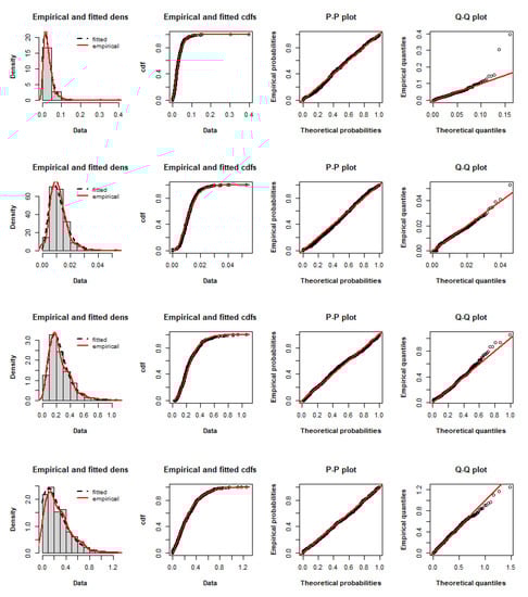
Figure 5. Empirical densities, empirical cdfs, P-P plots and Q-Q plots of the fitted MPoE distribution to the V19, V20, V28 and V29 sets.

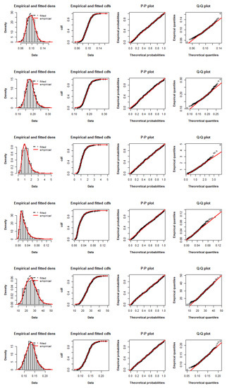
Figure 6. Empirical densities, empirical cdfs, P-P plots and Q-Q plots of the fitted MPoW distribution to the V7, V11, V14, V18, V24 and V27 sets.

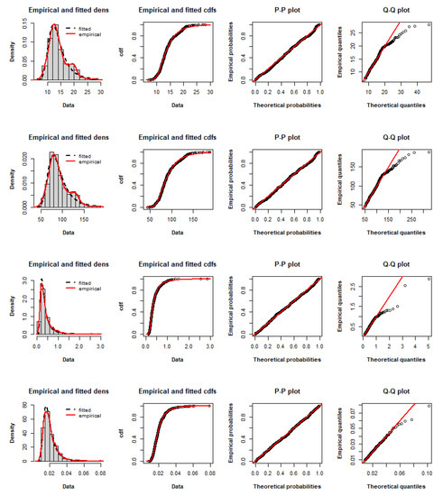
Figure 7. Empirical densities, empirical cdfs, P-P plots and Q-Q plots of the fitted MPoF distribution to the V3, V5, V13 and V21 sets.

4.2.2. Coal-Mining Data

The data set represents the time intervals in days between explosions in mines, involving more than 10 men killed in Great Britain, for the period 1875–1951, published by [27]. The data are:

1, 4, 4, 7, 11, 13, 15, 15, 17, 18, 19, 19, 20, 20, 22, 23, 28, 29, 31, 32, 36, 37, 47, 48, 49, 50, 54, 54, 55, 59, 59, 61, 61, 66, 72, 72, 75, 78, 78, 81, 93, 96, 99, 108, 113, 114, 120, 120, 120, 123, 124, 129, 131, 137, 145, 151, 156, 171, 176, 182, 188, 189, 195, 203, 208, 215, 217, 217, 217, 224, 228, 233, 255, 271, 275, 275, 275, 286, 291, 312, 312, 312, 315, 326, 326, 329, 330, 336, 338, 345, 348, 354, 361, 364, 369, 378, 390, 457, 467, 498, 517, 566, 644, 745, 871, 1312, 1357, 1613, 1630.

We fit the MPoE distribution to these data and compare with the exponential (Exp) distribution with rate parameter $\lambda$, the Weibull distribution with shape parameter a and scale parameter $\lambda$, the Marshall–Olkin exponential (MOE) distribution with parameters a and $\lambda$ as defined by [1], the exponentiated exponential (Exp-E) distribution with parameters a and $\lambda$ as given by [28], the gamma exponential I (GE-I) distribution as given by [11] and the log-expo exponential (LET-E) distribution as defined by [29].

Table 9 provides the MLEs and 95% CIs of the model parameters. Table 10 reports the adequacy of the models through a combination of several statistics (AIC, CAIC, BIC, HQIC, minus maximized log-likelihood function ($-\ell \left(\widehat{\theta }\right)$), Kolmogorov–Smirnov test statistic (KS) and its p-values), which measure the relative quality of fit of these models to a data set.

Table 9. Estimation results for coal mining data set.

Distribution	MLEs		95% CI
	$\widehat{\mathit{a}}$	$\widehat{\mathit{\lambda }}$	$\widehat{\mathit{a}}$	$\widehat{\mathit{\lambda }}$
MPoE	0.4477	0.0023	(−0.0468,0.9423)	(−0.0355,0.0401)
Exp	-	0.0043	-	(0.0035,0.0050)
Weibull	0.8848	218.68	(0.7588,1.0091)	(168.93,266.27)
MOE	0.5905	0.0033	(0.2512,0.8007)	(0.0021,0.0039)
Exp-E	0.8645	0.0040	(0.6604,1.0686)	(0.0030,0.0049)
GE-I	0.8780	0.0038	(0.6875,1.0684)	(0.0028,0.0049)
LET-E	1.1485	0.0027	(0.2253,2.0718)	(0.0019,0.0035)

Table 10. Adequacy measures for coal mining data set.

Distribution	AIC	CAIC	BIC	HQIC	$-\mathit{\ell }(\widehat{\mathit{a}},\widehat{\mathit{\lambda }})$	KS Test
						Statistic	p-Value
MPoE	1405.310	1405.423	1410.693	1407.493	700.6551	0.0641	0.7615
Exp	1408.627	1408.664	1411.318	1409.718	703.3133	0.0786	0.5107
Weibull	1407.545	1407.658	1412.927	1409.728	701.7724	0.0784	0.5135
MOE	1407.006	1407.119	1412.388	1409.188	701.5028	0.0700	0.6591
Exp-E	1409.135	1409.248	1414.517	1411.318	702.5673	0.0779	0.5222
GE-I	1408.898	1409.011	1414.280	1411.081	702.4489	0.0748	0.5748
LET-E	1406.484	1406.597	1411.867	1408.667	701.2419	0.0777	0.5257

Based on adequacy statistics introduced in Table 10, the MPoE model fits the data sets with minimum AIC, CAIC, BIC, HQIC, log-likelihood and maximum p-value among the other distributions. Thus, it can be a a good choice for modeling these data. This result is illustrated graphically in Figure 8 by comparing the empirical distribution of the data with the fitted MPoE distribution, respectively, by displaying (a) the histogram and fitted MPoE distribution, (b) the fitted MPoE survival function and the empirical survival (c) the P-P plot and (d) the Q-Q plot.

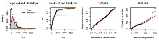
Figure 8. Empirical density, empirical cdf, P-P plot and Q-Q plot of the fitted MPoE distribution to coal-mining data.

5. Conclusions

We studied a new family of continuous distributions with a single extra parameter and showed its usefulness in practice by means of several applications. The new model is a mixture distribution, which can arise in a wide variety of fields. The new model is discussed from the weighted distributions’ viewpoint. Connections between measures of the new family and the parent distribution are addressed. The extra parameter boosted the flexibility of the family to cope with several types of data sets. We compare the proposed family with some distributions and special models generated from other classes using classical statistical measures. The new family can generate models that are powerful to represent and predict real-world data.

References

- Marshall, A.W.; Olkin, I. A New Method for Adding a Parameter to a Family of Distributions with Application to the Exponential and Weibull Families. Biometrika 1997, 84, 641–652. [Google Scholar] [CrossRef]
- Ghitany, M.E.; Al-Hussaini, E.K.; Al-Jarallah, R.A. Marshall-Olkin Extended Weibull Distribution and Its Application to Censored Data. J. Appl. Stat. 2005, 32, 1025–1034. [Google Scholar] [CrossRef]
- Ghitany, M.E.; Al-Awadh, F.A.; Alkhalfan, L.A. Marshall-Olkin Extended Lomax Distribution and Its Application to Censored Data. Commun. Stat. Theory Methods 2007, 36, 1855–1866. [Google Scholar] [CrossRef]
- Krishna, E.; Jose, K.K.; Alice, T.; Ristic, M.M. Marshall-Olkin Frechet Distribution. Commun. Stat. Theory Methods 2013, 42, 4091–4107. [Google Scholar] [CrossRef]
- Al-Saiari, A.Y.; Baharith, L.A.; Mousa, S.A. Marshall-Olkin Extended Burr Type XII Distribution. Int. J. Stat. Probab. 2014, 3, 78–84. [Google Scholar] [CrossRef] [Green Version]
- Okorie, I.E.; Akpanta, A.C.; Ohakwe, J.; Chikezie, D.C. The modified Power function distribution. Cogent Math. 2017, 4, 1319592. [Google Scholar] [CrossRef]
- Eugene, N.; Lee, C.; Famoye, F. Beta-Normal Distribution and Its Applications. Commun. Stat.-Theory Methods 2002, 31, 497–512. [Google Scholar] [CrossRef]
- Nadarajah, S.; Kotz, S. The Beta Exponential Distribution. Reliab. Eng. Syst. Saf. 2006, 91, 689–697. [Google Scholar] [CrossRef]
- Barreto-Souza, W.; Santos, A.H.S.; Cordeiro, G.M. The Beta Generalized Exponential Distribution. J. Stat. Comput. Simul. 2010, 80, 159–172. [Google Scholar] [CrossRef] [Green Version]
- Domma, F.; Condino, F. The Beta-Dagum Distribution: Definition and Properties. Commun. Stat. Theory Methods 2013, 42, 4070–4090. [Google Scholar] [CrossRef]
- Zografos, K.; Balakrishnan, N. On Families of Beta- and Generalized Gamma-Generated Distributions and Associated Inference. Stat. Methodol. 2009, 6, 344–362. [Google Scholar] [CrossRef]
- Cordeiro, G.M.; de Castro, M. A new family of generalized distributions. J. Stat. Comput. Simul. 2011, 81, 883–898. [Google Scholar] [CrossRef]
- Ristić, M.M.; Balakrishnan, N. The Gamma Exponentiated Exponential Distribution. J. Stat. Comput. Simul. 2012, 82, 1191–1206. [Google Scholar] [CrossRef]
- Amini, M.; MirMostafaee, S.; Ahmadi, J. Log-Gamma-Generated Families of Distributions. Stat. A J. Theor. Appl. Stat. 2013, 48, 913–932. [Google Scholar] [CrossRef]
- AL-Hussani, E.K. Composition of Cumulative Distribution Functions. J. Stat. Thoery Appl. 2012, 11, 323–336. [Google Scholar]
- Tahir, M.H.; Nadarajah, S. Parameter induction in continuous univariate distributions: Well-established G families. An. Acad. Bras. Ciênc 2015, 87, 539–568. [Google Scholar] [CrossRef] [PubMed]
- Barakat, H.M.; Khaled, O.M. Toward the establishment of a family of distributions that may fit any dataset. Commun. Stat. -Simul. Comput. 2017, 46, 6129–6143. [Google Scholar] [CrossRef]
- Mahdavi, A.; Kundu, D. A New Method for Generating Distributions with an Application to Exponential Distribution. Commun. Stat.-Theory Methods 2017, 46, 6543–6557. [Google Scholar] [CrossRef]
- Hussein, M.; Elsayed, H.; Cordeiro, G.M. A New Family of Continuous Distributions: Properties and Estimation. Symmetry 2022, 14, 276. [Google Scholar] [CrossRef]
- Patil, G.P. Weighted Distributions. In Wiley StatsRef: Statistics Reference Online; Wiley: Hoboken, NJ, USA, 2014. [Google Scholar]
- Rao, C.R. On Discrete Distributions Arising out of Methods of Ascertainment. Sankhyā Indian J. Stat. 1965, 27, 311–324. [Google Scholar]
- Gupta, R.C.; Kirmani, S.N.U.A. The role of weighted distributions in stochastic modeling. Commun. Stat.-Theory Methods 1990, 19, 3147–3162. [Google Scholar] [CrossRef]
- Saghir, A.; Hamedani, G.G.; Tazeem, S.; Khadim, A. Weighted Distributions: A Brief Review, Perspective and Characterizations. Int. J. Stat. Probab. 2017, 6, 109–133. [Google Scholar] [CrossRef] [Green Version]
- Jain, K.; Singh, H.; Bagai, I. Relations for reliability measures of weighted distributions. Commun. Stat.-Theory Methods 1987, 18, 4393–4412. [Google Scholar] [CrossRef]
- R Core Team. R: A Language and Environment for Statistical Computing; R Foundation for Statistical Computing: Vienna, Austria, 2020. [Google Scholar]
- William, H.; Wolberg, W.; Street, N.; Olvi, L. Mangasarian UCI Machine Learning Repository. Available online: http://archive.ics.uci.edu/ml (accessed on 12 September 2021).
- Maguire, B.A.; Pearson, E.S.; Wynn, A.H.A. The Time Intervals Between Industrial Accidents. Biometrika 1952, 39, 168–180. [Google Scholar] [CrossRef]
- Gupta, R.C.; Gupta, P.L.; Gupta, R.D. Modeling Failure Time Data by Lehman Alternatives. Commun. Stat.-Theory Methods 1998, 27, 887–904. [Google Scholar] [CrossRef]
- Aslam, M.; Ley, C.; Hussain, Z.; Shah, S.F.; Asghar, Z. A new generator for proposing flexible lifetime distributions and its properties. PLoS ONE 2020, 15, e0231908. [Google Scholar] [CrossRef] [PubMed]
Publisher’s Note: MDPI stays neutral with regard to jurisdictional claims in published maps and institutional affiliations. |
© 2022 by the authors. Licensee MDPI, Basel, Switzerland. This article is an open access article distributed under the terms and conditions of the Creative Commons Attribution (CC BY) license (https://creativecommons.org/licenses/by/4.0/).