Image Encryption Schemes Based on a Class of Uniformly Distributed Chaotic Systems

Abstract

This paper proposes a method to construct a one-dimensional discrete chaotic system. First, we define a generalized distance function to control the boundedness of the one-dimensional discrete system. Based on Marotto’s theorem, one-dimensional discrete systems are proven to be chaotic in the sense of Li–Yorke, and the corresponding chaos criterion theorem is proposed. The system can be distributed uniformly by adjusting the parameters. In this paper, we propose an image encryption scheme based on a uniformly distributed discrete chaotic system and DNA encoding. DNA encoding and decoding rules are determined by plain text. The experimental results demonstrate that our encryption algorithm has a large key space, high key sensitivity, and fast encryption speed and can resist differential and statistical attacks.

1. Introduction

Chaos is a special type of complex dynamic behavior displayed in nonlinear systems that commonly exists in nature, such as mathematics, physics, psychology, biology, and other fields. Chaotic systems have many essential properties, such as ergodicity, extreme sensitivity to initial conditions, and good pseudorandom behavior, which makes chaos theory a popular research subject. In recent years, chaotic systems have been rapidly developed and applied in many fields, especially electronic communications and cryptography [1,2]. As one of the most important information carriers, the security of images is very important and has drawn increasing attention from the public and researchers. However, due to a variety of intrinsic characteristics of images, such as a strong correlation of adjacent pixels, data redundancy, and high computational complexity, traditional encryption algorithms are unsuited to encrypt images. Therefore, researchers have proposed many image encryption algorithms [3,4,5]. Chaos-based image cryptosystems have become one of the most ideal encryption methods [6,7,8] because of the main features of chaotic systems, such as sensitivity to initial conditions, ergodicity, and highly complex behavior in addition to their mixing properties.

Researchers have been extensively attracted to constructing new chaotic systems in terms of the existing theory [9,10], which involves the discrimination for the existence of chaos in dynamical systems. In 1975, Li and Yorke first defined the term chaos from a mathematical perspective and proposed a criterion for the existence of chaos in one-dimensional discrete dynamical systems [11], which is well known as “period three implies chaos”. Under the guidance of Li–Yorke’s criterion, Marotto generalized a high-dimensional discrete dynamical system in 1978, which is known as Marotto’s theorem [12]. Shi and Chen proposed a new modified version of Marotto’s theorem [13] in 2005. Based on Li–Yorke’s criterion, a sufficient and necessary condition for the existence of the three periodic points of a quadratic polynomial is obtained by decomposing the real coefficient polynomial in a complex field [14]. A chaos criterion theorem on a cubic discrete system was established and proven to be chaotic in the sense of Li–Yorke [15]. Nevertheless, it is difficult to construct chaotic systems in terms of this criterion. Thus far, only a small number of related work has been reported. In contrast to Li–Yorke’s criterion, Marotto’s theorem appears more instrumental in proposing a theoretical direction. Based on Marotto’s theorem, Chen and Lai discussed an automatic control problem for discrete-time dynamical systems by adding a control term and then proposed an algorithm to control Lyapunov exponents for discrete-time dynamical systems, which is known as the Chen–Lai algorithm [16]. Moreover, several bounded functions containing modulus, sine, and saw-tooth functions were applied to globally bind the discrete system in the Chen–Lai algorithm, and the control term is a linear function [17]. To eliminate the linear control term in the Chen–Lai algorithm, a chaos criterion theorem for a one-dimensional discrete system was provided, in which a modulus function was used as a bounded function [18]. It is worth considering whether other bounded functions could lead to a similar proposition while eliminating linear control.

Low-dimensional chaotic maps have a simple structure and are easy to implement, but they usually have a small key space. In this paper, the proposed chaotic system overcomes the shortcomings of the traditional low-dimensional chaotic system with a small key space by adjusting parameters; therefore, a uniform distribution can be achieved.

DNA computing technology has attracted more and more attention since Adleman studied it [19]. Cryptography utilizes DNA as an information carrier in image encryption and has shown promising results by taking advantage of excellent DNA properties, such as massive parallelism, large storage, and ultralow power consumption. The authors of [20] proposed a color image encryption scheme based on DNA operations and a spatiotemporal chaotic system. The key stream of image encryption is associated with the key and plaintext image, which improves the ability to resist known plaintext or selected plaintext attack. Liu et al. [21] proposed color image encryption based on dynamic DNA and 4-D memristive hyperchaos. The main feature of the algorithm is that the dynamic DNA mechanism based on hyperchaos is performed on the processes of encoding, confusion, and diffusion, improving the security of the algorithm. Liu et al. [22] combined DNA computing with double-chaos systems composed of Lorenz chaotic mapping with variable parameters and fourth-order Rossler hyperchaotic mapping and proposed an algorithm for color image encryption at the bit level. The double-chaos system compensates for the pseudorandomness of the two types of chaotic mappings, making chaotic sequences more difficult to predict.

In this paper, a generalized distance function is defined as bounded, and it is applied to control the boundedness of a discrete system. In terms of Marotto’s theorem, a one-dimensional discrete system is discussed, and the corresponding chaos criterion theorem is set up to determine the existence of chaos in the discrete system. The system can be distributed uniformly by adjusting the parameters. An image encryption scheme is proposed based on this kind of uniformly distributed discrete chaotic system. First, the chaotic sequence is used to scramble and XOR transform the image, and then DNA coding and DNA operation are performed, the rules of which are determined by plain text. The remainder of this paper is organized as follows. Section 2 presents a class of uniformly distributed discrete chaotic systems and analyzes their dynamic behaviors. Image encryption based on DNA coding is proposed in Section 3. Section 4 gives the simulation experiment results and states security analyses. Finally, Section 5 concludes the paper.

2. A Class of Uniformly Distributed Chaotic Systems

2.1. Chen–Lai Algorithm

The Chen–Lai algorithm considers a nonlinear discrete system, not necessarily chaotic, of the form:

$$x_{k+1}=f_k(x_k), x_k\in R^n.$$

(1)

Then, a control input sequence ${\left\{u_k\right\}}_{k=0}^{\infty }$ is designed to investigate the automatic control of system (1), and a new system is described as:

$$x_{k+1}=f_k(x_k)+u_k, x_k\in R^n,$$

(2)

where $u_k=B_k{x}_k$ is discussed for short.

Assume the sequence $\left\{B_k\right\}$ is uniformly bounded:

$$\underset{0\le k<\infty }{\sup }\Vert B_k\Vert \le M<\infty$$

where $M$ is a positive constant and $\Vert \cdot \Vert$ denotes the spectral norm of a finite-dimensional matrix.

Under the only assumption, it is proven that, in practice, the algorithm can provide the required Lyapunov exponents and achieve the expected anti-control of system (2).

The Chen–Lai algorithm, based on the modulus, sine, and saw-tooth function, is further discussed in detail in [17]. Based on the modulus operation, the one-dimensional discrete system in the Chen–Lai algorithm has the form:

$$x_{k+1}=f(x_k)+u_k (\mathrm{mod}1),$$

(3)

where $u_k=(N+e^c)x_k$ is the control term and $N$ and $c$ are two constants.

A proposition is given on the one-dimensional discrete system (3) as follows.

Lemma 1.

[17] If$f(0)=0$, $c>0$ and $|f^{\prime }(x)|<1\le N$ are satisfied, then the controlled system (3) is chaotic in the sense of Li–Yorke.

The chaotic systems constructed by proposition 1 appear limited in having a linear control term; then, a one-dimensional system without a linear control term is considered with the form [18]:

$$x_{k+1}=f(x_k) (\mathrm{mod}1),$$

(4)

where $x_k\in R^1$, $f(x)\in C^1[0,1]$ and $f(0)=0$.

The chaos criterion theorem for system (4) is also provided.

Lemma 2.

[18] If$|f’(x)|>1$and$x\in [0,1)$are satisfied, then system (4) is chaotic in the sense of Li–Yorke.

Evidently, Lemma 1 is a special case of Lemma 2. In short, the form of system (3) is generalized to the form of system (4), while the bounded function is a modulus function. Naturally, under the guidance of the Chen–Lai algorithm and the work of proposition 2, a new bounded function can be defined to replace the modulus function and propose the corresponding chaos criterion theorem. This work is described in Section 2.2.

2.2. A One-Dimensional Discrete Chaotic System

This definition begins without describing the modified Marotto’s theorem, which is used later.

Lemma 3.

[13] Let$f:R\to R$be a map with a fixed point$z\in R^n$. Assume that

(1) 

f is continuously differentiable in a neighborhood of z and all the eigenvalues of$Df(z)$have absolute values larger than 1, which implies that there exists a positive constant$r$and a norm$\Vert \cdot \Vert$in$R^n$such that f is expanding in${\overline{B}}_r(z)$in$\Vert \cdot \Vert$, where${\overline{B}}_r(z)$is the closed ball of radius centered at z in$(R^n,\Vert \cdot \Vert )$;

(2) 

z is a snap-back repeller of f with$f^m(x_0)=z$,$x_0\ne z$, for some$x_0\in B_r(z)$and some positive integer m, where$B_r(z)$is the open ball of radius centered at z in$(R^n,\Vert \cdot \Vert )$. Furthermore, f is continuously differentiable in some neighborhoods of$x_0,x_1,\cdots ,x_{m-1}$, and$\det Df(x_j)\ne 0$for$0\le j\le m-1$, where$x_j=f(x_{j-1})$and$0\le j\le m-1$.

2.2.1. A Generalized Distance Function

First, a distance function is defined.

Definition 1.

Let$x\in R$; then, there exists an integer$N\in R$such that$x\in [N,N+1]$. A distance function as$f(x)=\min \{x-N,N+1-x\}$is defined. For simplicity, it is denoted as$f(x)\triangleq (x)$.

Absolutely, the function $f(x)\triangleq (x)$ is an even function. Then, a generalized distance function is further defined by adding a scale parameter into the distance function in Definition 1.

Definition 2.

A generalized distance function is defined as$Di{s}_{\epsilon }(x)=\epsilon \cdot (x)$, where parameter$\epsilon$is a positive constant.

The image of function $Di{s}_{\epsilon }(x)$ is displayed in Figure 1. Note that $Di{s}_{\epsilon }(x)\in [0,\epsilon /2]$ and it is also an even function.

Figure 1. Image of function $Di{s}_{\epsilon }(x)$.

2.2.2. Two Chaos Criterion Theorems

Theorem 1.

Consider a one-dimensional linear discrete system.

$$x_{k+1}=Di{s}_{\epsilon }(a{x}_k),a\ne 0.$$

(5)

If$\left|a\right|\epsilon \ge 2$is satisfied, then system (5) is a chaotic system in sense of Li–Yorke.

Proof of Theorem 1.

If $a<0$ is satisfied, then $x_{k+1}=Di{s}_{\epsilon }(a{x}_k)=Di{s}_{\epsilon }(-a{x}_k)$, which is actually $a>0$. Therefore, only $a>0$ is proved for simplicity.□

Denote $g(x)=Di{s}_{\epsilon }(ax)$. Then, while $0\le x\le 1/a$, $g(x)$ can be expressed as:

$$g(x)=\{\begin{array}{ll}a\epsilon x,& 0\le x<1/(2a)\\ \epsilon (1-ax),& 1/(2a)\le x\le 1/a\end{array}$$

The derivative of map $g(x)$ satisfies $|g^{\prime }(x)|=\left|a\right|\epsilon >1$, where $0\le x\le 1/a$ and $x\ne 1/(2a)$. In addition, condition $\left|a\right|\epsilon =a\epsilon \ge 2$ gives $1/a\le \epsilon /2$.

Denote $J_1=(0,1/(2a))$, $J_2=(1/(2a),1/2a)$.

In interval $J_2$, $g(x)=\epsilon (1-ax)=x$ gives a fixed point:

$$x^{*}=\frac{\epsilon }{1+a\epsilon }$$

Next, the fixed point $x^{*}$ is proven as a snap-back repeller.

A sequence $\left\{x_{-m}\right|m=0,1,2,\cdots \}$ is defined as:

$$x_0=\frac{1}{a(1+a\epsilon )}\in J_1, x_{-m}=\frac{\epsilon -x_{-m+1}}{a\epsilon }\in J_2, m=1,2,\cdots$$

Then, $x^{*}=g(x_0)=g^2(x_{-1})=\cdots =g^m(x_{-m+1})$.

By the Lagrange mean value theorem, there exists a point $\xi \in (x_{-m+1},x^{*})$ or $\xi \in (x^{*},x_{-m+1})$ such that:

$$|x_{-m+2}-x^{*}|=|g(x_{-m+1})-g(x^{*})|=|g^{\prime }(\xi )(x_{-m+1}-x^{*})|>|x_{-m+1}-x^{*}|$$

Hence, let the positive integer $m$ be large enough; then, there exists a constant $r>0$ such that:

$$x_{{}^{-m+1}}\in B_r(x^{*})\subset J_2, x_{{}^{-m+k}}\notin B_r(x^{*}), k=2,3,\cdots ,m$$

where $B_r(x^{*})=[x^{*}-r,x^{*}+r]$ is a closed ball and $g(x)$ is continuously differentiable in $B_r(x^{*})$.

In summary, the fixed point $x^{*}$ satisfies the following conditions:

(a) There exists a positive constant $r>0$ such that for any point $x\in B_r(x^{*})\subset J_2$,

$$\det \{Dg(x)\}=|g^{\prime }(x)|=\left|a\right|\epsilon =a\epsilon >1,$$

where $Dg(x)=g^{\prime }(x)$ denotes the Jacobi matrix of $g(x)$.

That is, the eigenvalue of $Dg(x)$ is $\lambda =g^{\prime }(x)$, and it satisfies $\left|\lambda \right|=|g^{\prime }(x)|=a\epsilon >1$.

(b) There exists a point $x_{{}^{-m+1}}\in B_r(x^{*})\subset J_2$ and a positive integer $m\ge 2$ such that $g^m(x_{-m+1})=x^{*}$, and

$$|\det \{D{g}^m(x_{-m+1})\}|=\left|{\displaystyle \prod _{i=1}^m\det \{Dg(x_{-i+1})\}}\right|={(a\epsilon )}^m\ne 0$$

In summary, $x^{*}$ is a snap-back repeller of system (5). This completes the proof.

In the proof of Theorem 1, the derivative of map $g(x)=Di{s}_{\epsilon }(ax)$ satisfies $|g^{\prime }(x)|=\left|a\epsilon \right|>2$, which shows that the Lyapunov exponent of system (5) is $\lambda =\ln \left|a\epsilon \right|>0$.

Theorem 2.

Consider a one-dimensional nonlinear discrete system

$$x_{k+1}=Di{s}_{\epsilon }(f(x_k)),$$

(6)

where$f(x)\in C^1[0,\epsilon /2]$ and$f(0)=0$.

If$|f^{\prime }(x)|>1$,$x\in [0,\epsilon /2]$ and$\epsilon \ge 2$, then system (6) is chaotic in the sense of Li–Yorke.

Proof of Theorem 2.

Assume $|f^{\prime }(x)|>1$ gives $f^{\prime }(x)>1$ or $f^{\prime }(x)<-1$.□

If $f^{\prime }(x)<-1$ is satisfied, then $x_{k+1}=Di{s}_{\epsilon }(f(x_k))=Di{s}_{\epsilon }(-f(x_k))$, which is actually $f^{\prime }(x)>1$. Therefore, only $f^{\prime }(x)>1$ is proved for simplicity.

Denote $g(x)=Di{s}_{\epsilon }(f(x))$, then its derivative satisfies $|g^{\prime }(x)|=|Di{s_{\epsilon }}^{\prime }(x)f^{\prime }(x)|=\epsilon f^{\prime }(x)>1$.

By the Lagrange mean value theorem, there exists a point $\xi \in [0,x]$ such that

$$f(x)=f(x)-f(0)=f^{\prime }(\xi )x>x$$

which gives $f(1/2)>1/2$ and $f(1)>1$.

Since $f(1/2)>1/2>0=f(0)$, there exists a point $t_0\in (0,1/2)$ such that $f(t_0)=1/2$.

Since $f(1)>1>1/2=f(t_0)$, there exists a point $t_1\in (t_0,1)$ such that $f(t_1)=1$.

The monotonicity of map $f(x)$ ensures the uniqueness of points $t_0$ and $t_1$.

Then, $g(t_0)=Di{s}_{\epsilon }(f(t_0))=\epsilon /2$ and $g(t_1)=Di{s}_{\epsilon }(f(t_1))=0$.

Denote $h(x)=g(x)-x$, and $\epsilon \ge 2$ gives

$$h(t_0)=g(t_0)-t_0=\epsilon /2-t_0>0,h(t_1)=g(t_1)-t_1=-t_1<0$$

which indicates there exists a point $x^{*}\in (t_0,t_1)$ such that $h(x^{*})=0$. Moreover, $h^{\prime }(x)=g^{\prime }(x)-1>0$.

Absolutely, point $x^{*}$ is a fixed point of map $g(x)$ in interval $(t_0,t_1)$.

Next, the fixed point $x^{*}$ is proven to be a snap-back repeller.

Since $g(0)=0<x^{*}<\epsilon /2=g(t_0)$, there exists a point $x_0\in (0,t_0)$ such that $g(x_0)=x^{*}$.

Since $g(t_1)=0<x_0<x^{*}=g(x^{*})$, there exists a point $x_{-1}\in (x^{*},t_1)$ such that $g(x_{-1})=x_0$.

Since $g(x^{*})=x^{*}<x_{-1}<\epsilon /2=g(t_0)$, there exists a point $x_{-2}\in (t_0,x^{*})$ such that $g(x_{-2})=x_{-1}$.

Since $g(t_1)=0<x_{-2}<x^{*}=g(x^{*})$, there exists a point $x_{-3}\in (x^{*},t_1)$ such that $g(x_{-3})=x_{-1}$.

Therefore, it can be proven that there exists a point $x_{-m+1}\in (t_0,x^{*})$ or $x_{-m+1}\in (x^{*},t_1)$ such that $g(x_{-m+1})=x_{-m+2}$.

Then, $x^{*}=g(x_0)=g^2(x_{-1})=\cdots =g^m(x_{-m+1})$.

By the Lagrange mean value theorem, there exists a point $\xi \in (x_{-m+1},x^{*})$ or $\xi \in (x^{*},x_{-m+1})$ such that

$$|x_{-m+2}-x^{*}|=|g(x_{-m+1})-g(x^{*})|=|g^{\prime }(\xi )(x_{-m+1}-x^{*})|>|x_{-m+1}-x^{*}|.$$

Hence, let the positive integer m be large enough; then, there exists a constant $r>0$ such that

$$x_{{}^{-m+1}}\in B_r(x^{*})\subset (t_0,t_1),x_{{}^{-m+1}}\notin B_r(x^{*}),k=2,3,\cdots ,m$$

where $B_r(x^{*})=[x^{*}-r,x^{*}+r]$ is a closed ball and $g(x)$ is continuously differentiable in $B_r(x^{*})$.

In summary, the fixed point $x^{*}$ satisfies the following conditions:

(a) There exists a positive constant $r>0$ such that for any point

$$x\in B_r(x^{*})\subset (t_0,t_1), \det \{Dg(x)\}=|g^{\prime }(x)|=\epsilon f^{\prime }(x)>1,$$

where $Dg(x)=g^{\prime }(x)$ denotes the Jacobi matrix of $g(x)$.

That is, the eigenvalue of $Dg(x)$ is $\lambda =g^{\prime }(x)$, and it satisfies $\left|\lambda \right|=|g^{\prime }(x)|=\epsilon f^{\prime }(x)>1$.

(b) There exists a point $x_{{}^{-m+1}}\in B_r(x^{*})\subset (t_0,t_1)$ and a positive integer $m\ge 2$ such that $g^m(x_{-m+1})=x^{*}$, and

$$|\det \{D{g}^m(x_{-m+1})\}|=\left|{\displaystyle \prod _{i=1}^m\det \{Dg(x_{-i+1})\}}\right|={(\epsilon f^{\prime }(x))}^m\ne 0.$$

In summary, $x^{*}$ is a snap-back repeller of system (6). This completes the proof.

Theorem 2 cannot contain Theorem 1 while setting $f(x)=ax$ in Theorem 2.

2.2.3. Three Specific Propositions

To explain the application of Theorem 2, three propositions, based on Theorem 2, are proposed by designing the form of $f(x)$ in system (6).

Proposition 1.

Consider a one-dimensional discrete system

$$x_{k+1}=Di{s}_{\epsilon }(x_k{}^2+a{x}_k)=Di{s}_{\epsilon }(f(x_k)),$$

(7)

where$f(x)=x^2+ax$and$\epsilon \ge 2$. If$a>1$or$a<-\epsilon -1$, then system (7) is chaotic.

Note that$|f^{\prime }(x)|=|2x+a|>1$and$x\in [0,\epsilon /2]$give$a>1$or$a<-\epsilon -1$.

Proposition 2.

Consider a one-dimensional discrete system

$$x_{k+1}=Di{s}_{\epsilon }(a_n{x}_k^n+a_{n-1}{x}_k^{n-1}+\cdots +a_1{x}_k)=Di{s}_{\epsilon }(f(x_k)),$$

(8)

where$f(x)=a_n{x}^n+a_{n-1}{x}^{n-1}+\cdots +a_{1}x$and$\epsilon \ge 2$. If$|f^{\prime }(x)|>1$,$x\in [0,\epsilon /2]$, then system (8) is chaotic.

Especially, if set$a_i>0$,$i=2,3,\cdots ,n$and$a_1>1$, then$f^{\prime }(x)=a_n{x}^{n-1}+\cdots +a_{2}x+a_1>1$,$x\in [0,\epsilon /2]$. That is, system (8) is chaotic.

Proposition 3.

Consider a one-dimensional discrete system

$$x_{k+1}=Di{s}_{\epsilon }\left({\displaystyle {\int }_0^{x_k}g(t)dt}+a{x}_k\right)=Di{s}_{\epsilon }(f(x_k)),$$

(9)

where$f(x)={\displaystyle {\int }_0^{x}g(t)dt}+ax$,$g(x)\in C^1[0,\epsilon /2]$and$\epsilon \ge 2$. If$g(x)>0$,$x\in [0,\epsilon /2]$and$a>1$, then system (9) is chaotic. Note that$f^{\prime }(x)=g(x)+a>0+1=1$,$x\in [0,\epsilon /2]$and$f(0)=0$.

2.3. Dynamical Properties Analysis

In this section, the dynamic properties of chaotic systems in Theorems 1 and 2 will be analyzed by means of numerical simulations, such as bifurcation diagrams, and Lyapunov exponent spectra. Bifurcation diagrams describe the process in which states of nonlinear systems change when one parameter changes. An examination of Lyapunov exponents and bifurcation diagram together proved the existence of the chaotic behavior feature.

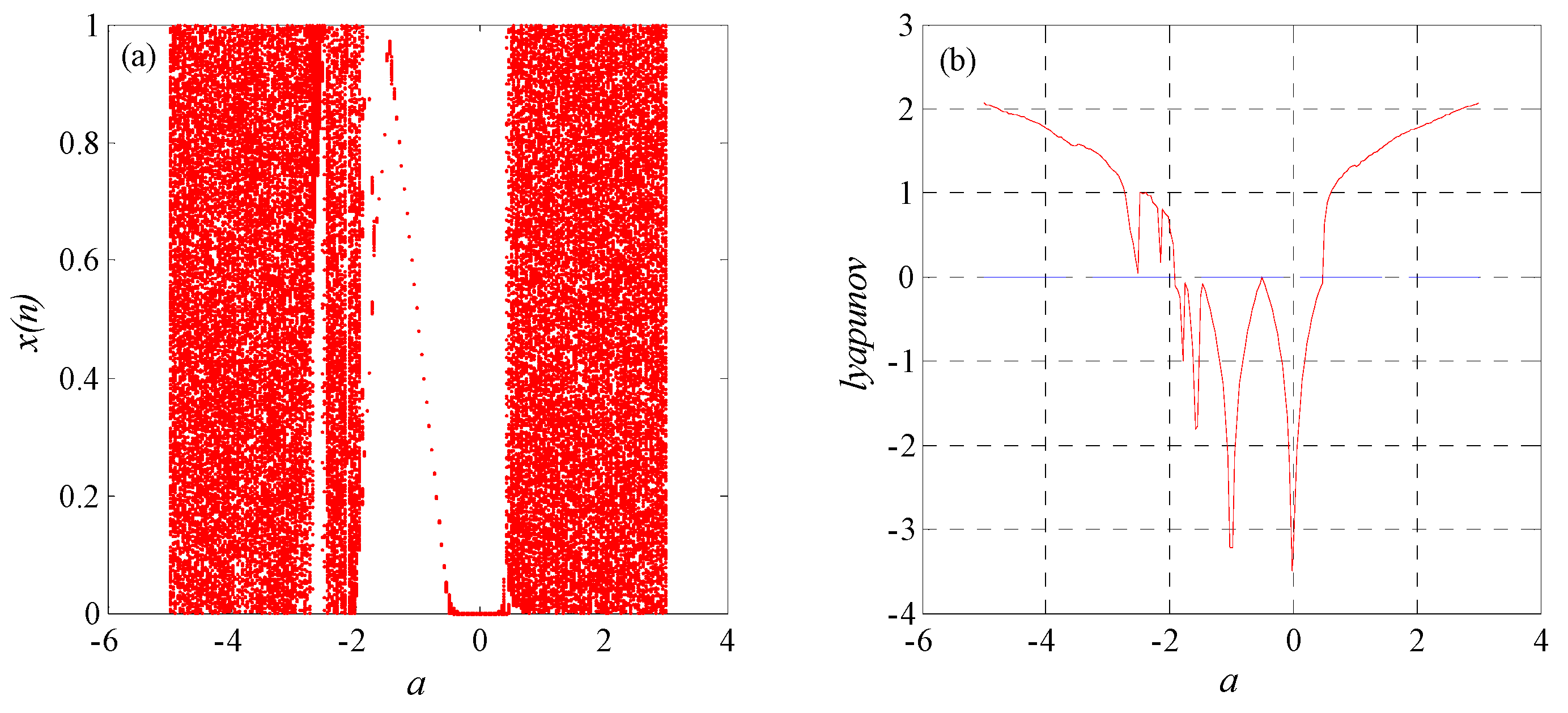
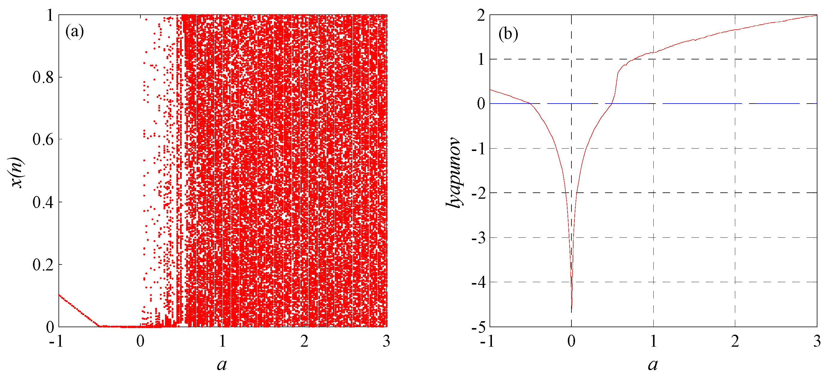
2.3.1. Bifurcation Diagrams and Lyapunov Exponent Spectra

In Theorem 1, let $\epsilon =2$; then, if $\left|a\right|\ge 1$, system (5) is chaotic in the sense of Li–Yorke. Let $a=1$; then, if $\epsilon \ge 2$, system (5) is chaotic in the sense of Li–Yorke.

Figure 2a,b show the bifurcation diagram and Lyapunov exponent spectrum of parameterin system (5) respectively, where. Figure 2c,d show the bifurcation diagram and Lyapunov exponent spectrum of parameterin system (5) respectively, where. As shown in Figure 2, system (5) displays its chaotic characteristics as theorem 1 expects.

Figure 2. Bifurcation diagrams and Lyapunov exponent spectra of system (5). Let $\epsilon =2$: (a) bifurcation diagram of a and (b) Lyapunov exponent spectrum of a. Let $a=1$: (c) bifurcation diagram of $\epsilon$ and (d) Lyapunov exponent spectrum of $\epsilon$.

In Proposition 1, let $\epsilon =2$; then, if or, system (7) is chaotic. The bifurcation diagram and Lyapunov exponent spectrum of the parameter in system (7) are shown in Figure 3a,b, respectively. Figure 3 shows that system (7) displays chaotic characteristics as expected by Proposition 1.

Figure 3. System (7): (a) bifurcation diagram of $a$ and (b) Lyapunov exponent spectrum of $a$.

In Proposition 3, set $g(x)=\sin (x)+1$; then, if $a>1$, system (9) is chaotic. The bifurcation diagram and Lyapunov exponent spectrum of parameter a in system (9) are shown in Figure 4a,b, respectively. Figure 4 shows that system (9) displays chaotic characteristics expected by Proposition 3.

Figure 4. System (9): (a) bifurcation diagram of $a$ and (b) Lyapunov exponent spectrum of $a$.

2.3.2. Correlation Analysis

In this subsection, we set $a=1$, $\epsilon =3$, $x_0=0.2759$ in system (5).

We set $a=2$, $\epsilon =2$, $x_0=0.2759$ in system (7).

The evolution of the state variable $k-x(k)$ in systems (5) and (7) for the first 3000 iterations is shown in Figure 5a,b, respectively. The dynamic behaviors of chaotic systems (5) and (7) all demonstrate chaotic attractors.

Figure 5. The evolution of the state variable: (a) system (5) and (b) system (7).

Autocorrelation and cross-correlation are two main methods to measure the pseudorandomness of chaotic systems. For a truly random series such as white noise, the autocorrelation and cross-correlation are the $\delta$ function and zero, respectively.

The autocorrelation coefficient at lag $k$ of a series $\{x(n)\}$ of length $N$ is normally given as:

$$autocorr(k)=\frac{{\displaystyle \sum _{i=1}^N(x(i)-\overline{x})(x(i+k)-\overline{x})}}{{\displaystyle \sum _{i=1}^N{(x(i)-\overline{x})}^2}},$$

where $\overline{x}$ is the mean of the series $\{x(n)\}$.

The cross-correlation of two series $\{x(n)\}$ and $\{y(n)\}$ of length $N$ at lag $k$ is defined as:

$$crosscorr(k)=\frac{{\displaystyle \sum _{i=1}^N(x(i)-\overline{x})(y(i-k)-\overline{y})}}{\sqrt{{\displaystyle \sum _{i=1}^N{(x(i)-\overline{x})}^2}}\sqrt{{\displaystyle \sum _{i=1}^N{(y(i)-\overline{y})}^2}}}.$$

For system (5), the autocorrelation function of the chaotic sequence generated with the initial parameters $a=1$, $\epsilon =3$, and $x_0=0.2759$ is shown in Figure 6a, and its cross-correlation with another chaotic system generated with $a=1$, $\epsilon =3$, and $x_0=0.3257$ is shown in Figure 6b.

Figure 6. System (5): (a) autocorrelation function and (b) cross-correlation function. System (7): (c) autocorrelation function and (d) cross-correlation function.

For system (7), the autocorrelation function of chaotic sequence generated with initial parameter $a=2$, $\epsilon =2$, $x_0=0.2759$ is shown in Figure 6c and its cross-correlation with another chaotic system generated with $a=2$, $\epsilon =2$, $x_0=0.3257$ is shown in Figure 6d.

Figure 6 shows that the autocorrelation and cross-correlation functions of the chaotic systems generated by systems (5) and (7) are all ideal, as expected, which means that their pseudorandomness is very close to that of a truly random sequence.

2.3.3. Distribution Density Analysis

In practical applications, the distribution density of chaotic systems is usually required to be uniform or nearly uniform. In this section, the distribution density of chaotic systems based on Theorems 1 and 2 is investigated by means of histograms. First, the simulation method of the chaotic system distribution density is described as follows.

Step 1 First, $\{x(n)\}$ is denoted as a chaotic sequence of length $N$ generated by a chaotic system. Assume the value range $\{x(n)\}$ of is $\Delta =[\alpha ,\beta ]$. In fact, $\alpha =\min \left\{x\right\{n\left\}\right\}$, $\beta =\max \left\{x\right\{n\left\}\right\}$.

Step 2 The interval $\Delta$ is divided into $M$ subintervals equally, and the length of each subinterval is $h=(\beta -\alpha )/M$.

Step 3 The number of samples that fall into each subinterval is counted and denoted as $n_i$, $i=1,2,\cdots ,M$.

Step 4 The probability of every point in the subinterval is denoted as $p_i$, $i=1,2,\cdots ,M$. Then, probability $p_i$ can be approximated by:

$$p_i=\frac{n_i}{N{\Delta }_i}.$$

Thus, ${\displaystyle \sum _{i=1}^N{p}_i{\Delta }_i}=1$.

Then, the distribution density of a chaotic system can be simulated by the corresponding probability histogram in terms of the above method. In the following simulation, without specific declaration, $N={10}^6$, $M=500$.

In Theorem 1, let $a=1$; then, $\epsilon =3$, $\epsilon =3.3$, $\epsilon =3.8$, and $\epsilon =3.99$ are set, and histograms of the chaotic sequences generated by system (5) are shown in Figure 7a–d.

Figure 7. Histogram of system (5) with $a=1$: (a) $\epsilon =3$; (b) $\epsilon =3.3$; (c) $\epsilon =3.8$; and (d) $\epsilon =3.99$.

In each histogram, the simulation represents the approximate value of probability $p_i$, and the curve $p(x)=2/\epsilon$ is used to fit the simulation of the distribution density of chaotic systems. Figure 7 shows that the distribution density of system (5) can be close to a uniform distribution by varying the system parameters, as shown in Figure 5a,d.

In fact, if set $a=1$ and $\epsilon =2$, the linear system (5) is a tent map that follows a uniform distribution. It can be verified that if $\left|a\epsilon \right|\ge 2$ is an integer, system (5) follows a uniform distribution in terms of the proof of the tent map. Now, the distribution density of nonlinear system (6) is studied, and for simplicity, system (7) is utilized as an example to study this problem.

Without loss of generality, we set $\epsilon =2$ in system (7) and then set $a=1$, $a=1.5$, $a=1.8$, and $a=2$, respectively, and histograms of the chaotic sequences generated by system (7) are shown in Figure 8a–d. As shown in Figure 8, the distribution density of system (7) can also be close to the uniform distribution by varying the system parameters.

Figure 8. Histogram of system (7) where $\epsilon =2$: (a) $a=1$; (b) $a=1.5$; (c) $a=1.8$; and (d) $a=2$.

3. The Proposed Image Encryption Scheme

3.1. DNA Encoding and Computing Rules

A DNA sequence consists of four basic nucleic acids: A (adenine), C (cytosine), G (guanine), and T (thymine). According to the pair rules, A and T are complementary, as are C and G. In the binary system, 0 and 1 are complementary. Therefore, binary numbers 00 and 11, and 10 and 01 are also complementary. If we use the four basic nucleic acids (i.e., A, C, G, T) to denote the four binary numbers 00, 01, 10, and 11, there are in total 4! = 24 kinds of encoding rules. However, only eight rules which satisfy the Watson–Crick complementary requirement are valid. The rules are shown in Table 1.

Table 1. DNA encoding rules.

Rule	Rule 1	Rule 2	Rule 3	Rule 4	Rule 5	Rule 6	Rule 7	Rule 8
00	A	A	T	T	C	C	G	G
01	G	C	C	G	A	T	A	T
10	C	G	G	C	T	A	T	A
11	T	T	A	A	G	G	C	C

According to the rules of DNA encoding and decoding, DNA sequences can be computed using algebraic calculation, such as addition, subtraction, and XOR operations. Table 2 lists the three operations for DNA sequences according to Rule 1.

Table 2. DNA computing rules.

+	A	G	C	T
A	A	G	C	T
G	G	C	T	A
C	C	T	A	G
T	T	A	G	C
-	A	G	C	T
A	A	T	C	G
G	G	A	T	C
C	C	G	A	T
T	T	C	G	A
XOR	A	G	C	T
A	A	G	C	T
G	G	A	T	C
C	C	T	A	G
T	T	C	G	A

3.2. Iterations of Chaotic Systems

For chaotic system (5), we take three group parameters $\left\{a_1,x_{01}\right\},$ $\left\{a_2,x_{02}\right\},$ and $\left\{a_3,x_{03}\right\},$ and iterate $N_0+MN$ times. In order to avoid the harmful effect of the transition procedure, we discard the previous $N_0$ sequence value and we obtain three chaotic sequences of length $M\times N$:

$$\begin{array}{l}{X}_1=\left\{x_1(i),i=1,2,\dots ,M\times N\right\}\\ X_2=\left\{x_2(i),i=1,2,\dots ,M\times N\right\}\\ X_3=\left\{x_3(i),i=1,2,\dots ,M\times N\right\}\end{array}$$

The sequence values of the first group of chaotic sequences $X_1$ are sorted from small to large, and the corresponding subscript sequences are recorded to obtain an ordered subscript sequence $X{P}_1=\left\{x{p}_1(i),i=1,2\dots M\times N\right\}$. For example, the sequence value of $x{p}_1(3)$ in $X{P}_1$ is 18, which means that the sequence number $x_1(3)$ of the sequence value in the chaotic sequence $X_1$ in the whole sequence $X_1$ is 18.

Similarly, the ordered subscript sequence $X{P}_2$ of chaotic sequence $X_2$ can be obtained.

The third group of chaotic sequences $X_3$ is transformed into an integer column r between [0, 255].

$$r=\mathrm{mod}\left(ceil\left(x_3\times {10}^8\right),256\right)$$

The integer column r is arranged in rows into a matrix with size $M\times N$, which is recorded as R;

For chaotic system (8), two sets of parameters $\left\{b_1,b_2,b_3,b_4,b_5,b_6,x_{04}\right\}$, $\left\{c_1,c_2,c_3,c_4,c_5,c_6,x_{05},\right\}$ are taken and iterated $N_0+MN$ times. Discarding the previous $N_0$ sequence value, we obtain two chaotic sequences of length $M\times N$:

$$\begin{array}{l}{X}_4=\left\{x_4(i),i=1,2,\dots ,M\times N\right\}\\ X_5=\left\{x_5(i),i=1,2,\dots ,M\times N\right\}\end{array}$$

The chaotic sequences $X_4$ and $X_5$ are transformed into two pseudorandom sequences between [0, 255]:

$$\begin{array}{l}{x}_4(i)=\mathrm{mod}\left(floor\left(\frac{L(x_4(i)-\min (x_4))}{\max (x_4)-\min (x_4)}\right),256\right)\\ x_5(i)=\mathrm{mod}\left(floor\left(\frac{L(x_5(i)-\min (x_5))}{\max (x_5)-\min (x_5)}\right),256\right)\end{array}$$

where $L=255\sqrt{2}\times {10}^8$ is a constant.

3.3. Proposed Image Encryption Scheme

Suppose the plain image is $P={\left(p\left(i,j\right)\right)}_{M\times N},i=1,2\dots M,j=1,2\dots N$.

Step 1: Convert the image matrix P into a one-dimensional array and the pixel position of the image $P$ is transformed by using the ordered subscript sequence $X{P}_1$ to obtain the image $P_1$.

Step 2: The image $P_1$ is divided into blocks and N pixels are taken in turn as a group to obtain M subimage $P{R}_i=\left\{p{r}_i(j),j=1,2,\dots ,N\right\},i=1,2,\dots ,M$.

Step 3: Combined with chaotic sequence $X_4$, the pixel value of each subimage $P{R}_i$ is transformed forward to obtain the subimage $PR{N}_i=\left\{pr{n}_i(j),j=1,2,\dots ,N\right\}$. The specific transformation is:

$$\begin{array}{l}pr{n}_i(j)=p{r}_i\left(j\right)\oplus x_4\left(\left(i-1\right)N+j\right)\oplus k_{i-1},j=1,2,\dots ,N,i=1,2\dots M,\\ k_i=pr{n}_i(1)\oplus pr{n}_i(2)\oplus \dots \oplus pr{n}_i(N),i=1,2\dots M-1,\end{array}$$

where $\oplus$ represents XOR operation, $k_0=\mathrm{mod}\left({\displaystyle \sum _i^M{\displaystyle \sum _j^{N}p{r}_i(j)+i+j,256}}\right)$ as a key.

Step 4: All pixel values in each subimage $PR{N}_i$ are shifted to the left circularly in bits, and the moving bit is $d\in \left\{1,2,\dots ,8\right\}$ to obtain the subimage $PR{B}_i=\left\{pr{b}_i(j),j=1,2,\dots ,N\right\}$. The specific transformation is:

$$pr{b}_i\left(j\right)=\mathrm{mod}\left(pr{n}_i\left(j\right)\times 2^d,256\right)+floor\left(pr{n}_i\left(j\right)/2^{8-d}\right)$$

Step 5: Combined with chaotic sequence $X_5$, the pixel value of each subimage $PR{B}_i$ is inversely transformed to obtain a new subimage $PR{C}_i$. The specific transformation is:

$$\begin{array}{c}pr{c}_i(j)=pr{b}_i\left(j\right)\oplus x_5\left(\left(i-1\right)N+j\right)\oplus l_{i-1},j=N,N-1,\dots ,1,i=M,M-\mathrm{1...1},\\ l_{i-2}=pr{c}_i(1)\oplus pr{c}_i(2)\oplus \dots \oplus pr{c}_i(N),i=M,M-\mathrm{1...2},\end{array}$$

where $l_{M-1}=\mathrm{mod}\left({\displaystyle \sum _i^M{\displaystyle \sum _j^{N}pr{b}_i(j)+i+j,256}}\right)$ as a key.

Step 6: The $PR{C}_i$ subimages are spliced to obtain the image $P_2$, and the pixel position of the image $P_2$ is transformed by the ordered subscript sequence $X{P}_2$. The transformed image $P_3$ is rearranged into an image of size $M\times N$.

Step 7: The image $P_3$ is encoded as a DNA matrix, and the matrix R in Section 3.2 is also encoded as a DNA matrix. The two DNA matrices are operated, the calculated DNA matrix is decoded to obtain a binary matrix, and finally, it is converted into a decimal matrix, that is, the last ciphertext image. The encoding and decoding rules and operation rules in the step are determined by the plaintext image. The calculation formula of encoding, decoding, and operation rules is as follows:

$$\begin{array}{l}{r}_b=\mathrm{mod}\left(floor(sum(P)\ast 0.68),8\right)+1\\ r_r=\mathrm{mod}\left((sum(P)+i+j),8\right)+1\\ r_y=\mathrm{mod}\left(sum(P),3\right)\\ r_j=\mathrm{mod}\left(ceil(sum(P)/126),8\right)+1\end{array}$$

where $sum(P)$ represents the sum of pixel values of image P, $r_b$ represents the coding rules of image $P_3$, $r_r$ represents the coding rules of matrix R, $r_y$ represents the operation rules, and $r_j$ represents the decoding rules.

The encryption process can be described by Figure 9.

Figure 9. Image encryption scheme.

The decryption algorithm is the reverse process of the encryption algorithm.

4. Simulation Results and Security Analysis

We used MATLAB 2016a to verify the proposed encryption algorithm on a personal computer with an Intel(R) Core(TM) i7-7500U CPU @ 2.70 GHz and 8.00 GB memory, and the operating system was a Microsoft Windows 10. The test images are Lena (256 × 256), Girl(256 × 256), and Baboon(256 × 256). The system parameters of the chaotic system are

$$\left\{\begin{array}{c}{a}_1=2,x_{01}=0.2759,a_2=1.5,x_{02}=0.3257,a_3=2,x_{03}=0.28,\\ b_1=2,b_2=b_3=b_4=b_5=b_6=1,x_{04}=0.6871,\\ c_1=3,c_2=2,c_3=c_4=c_5=c_6=1,x_{05}=0.4179\\ n_0=1000,d=3\end{array}\right\}$$

The simulation results are shown in Figure 10.

Figure 10. Images encryption and decryption effect: (a,d,g) original image; (b,e,h) encrypted image; and (c,f,i) decrypted image.

4.1. Key Space Analysis

Key space measures the ability to resist exhaustive attacks. The key space size needs to be analyzed and calculated in combination with the system parameters involved in encryption, initial value conditions, and computer accuracy. Generally, the more key parameters there are, the greater the sensitivity of the key, the larger the key space, and the more difficult it is for the encryption and decryption algorithm to crack. In many other studies, the calculation accuracy is usually 10⁻¹⁴. Therefore, this paper sets the calculation accuracy to 10⁻¹⁴ to compare with the key space of the same scale.

The key space of this algorithm is ${\left({10}^{14}\right)}^{20}={10}^{280}$. Since the keys $\left\{n_0,k_0,l_{M-1},d,e,f,g,h\right\}$ are numbers in the integer field, the key space is not taken into account when calculating. Therefore, the key space of this algorithm is much larger than the minimum value of resisting violent attacks and the key space in the following references. The comparison with the key space in other references is provided in Table 3.

Table 3. Key space analysis.

	Ref. [23]	Ref. [24]	Ref. [25]	Ref. [26]	Proposed
Key space	${10}^{93}$	${10}^{98}$	${10}^{84}$	${10}^{142}$	${10}^{280}$

4.2. Key Sensitivity Analysis

A good encryption scheme should be sensitive to the key in the encryption process. Below, the key is slightly disturbed, and NPCR and UACI are used to measure the differences of the images before and after the perturbation.

The NPCR and UACI are expressed as follows:

$$\mathrm{NPCR}=\frac{{\displaystyle \sum _{\mathrm{i}=1}^{\mathrm{W}}{\displaystyle \sum _{\mathrm{j}=1}^{\mathrm{H}}\mathrm{D}(\mathrm{i},\mathrm{j})}}}{\mathrm{W}\times \mathrm{H}}\times 100\%,$$

$$\mathrm{UACI}=\frac{{\displaystyle \sum _{\mathrm{i}=1}^{\mathrm{W}}{\displaystyle \sum _{\mathrm{j}=1}^{\mathrm{H}}\frac{\left|{\mathrm{p}}_1(\mathrm{i},\mathrm{j})-{\mathrm{p}}_2(\mathrm{i},\mathrm{j})\right|}{\mathrm{L}-1}}}}{\mathrm{W}\times \mathrm{H}}\times 100\%,$$

$$D(i,j)=\{\begin{array}{l}0,p_1(i,j)=p_2(i,j)\\ 1,p_1(i,j)\ne p_2(i,j)\end{array},$$

where W × H is the number of pixels.

The key sensitivity analysis results of the encryption algorithm are shown in Table 4. The values of NPCR and UACI are very close to the ideal values of 99.609% and 33.464%, respectively, after a minor disturbance of the parameters. Therefore, there are large differences in decrypted images and high key sensitivity.

Table 4. Key sensitivity analysis.

Initial Parameters	Minor Disturbance	NPCR	UACI
$a_1$	$+{10}^{-14}$	99.63%	33.51%
$x_{01}$	$+{10}^{-14}$	99.61%	33.45%
$a_2$	$+{10}^{-14}$	99.62%	33.49%
$x_{02}$	$+{10}^{-14}$	99.60%	33.52%
$a_3$	$+{10}^{-14}$	99.60%	33.45%
$x_{03}$	$+{10}^{-14}$	99.62%	33.46%
$b_1$	$+{10}^{-14}$	99.59%	33.47%
$b_2$	$+{10}^{-14}$	99.62%	33.47%
$b_3$	$+{10}^{-14}$	99.60%	33.44%
$b_4$	$+{10}^{-14}$	99.63%	33.47%
$b_5$	$+{10}^{-14}$	99.61%	33.45%
$b_6$	$+{10}^{-14}$	99.61%	33.38%
$x_{04}$	$+{10}^{-14}$	99.61%	33.40%
$c_1$	$+{10}^{-14}$	99.58%	33.47%
$c_2$	$+{10}^{-14}$	99.60%	33.39%
$c_3$	$+{10}^{-14}$	99.62%	33.45%
$c_4$	$+{10}^{-14}$	99.59%	33.45%
$c_5$	$+{10}^{-14}$	99.62%	33.44%
$c_6$	$+{10}^{-14}$	99.60%	33.45%
$x_{05}$	$+{10}^{-14}$	99.61%	33.48%

4.3. Histogram Analysis

The statistical histogram directly observes the encryption effect of image encryption and reflects the distribution of pixels by comparing the pixel statistical histogram of the original image with the encrypted image. It is generally considered that the statistical histogram of an encrypted image is approximately uniform. Figure 11 shows the encrypted histogram of the Lena image. The histogram distribution is flat and better hides the statistical law of pixels. It can effectively resist statistical attacks and pure password attacks.

Figure 11. The result of Lena histogram analysis: (a) original image; (b) encrypted image; and (c) decrypted image.

4.4. Correlation Analysis

The correlation coefficient calculates the correlation coefficient of the original image and the encrypted image, compares the absolute value of the correlation coefficient, judges the correlation change of adjacent pixels of the encrypted image, and measures the correlation of adjacent pixels.

In digital images, the gray values between adjacent pixels are often very close, indicating that adjacent pixels have a strong correlation, which will lead to insufficient encryption security performance. When the absolute value of the correlation coefficient is close to 1, it is considered that there is a strong correlation between adjacent pixels; when the absolute value of the correlation coefficient is close to 0, it is considered that there is no or weak correlation between adjacent pixels. The calculation of the correlation coefficient between adjacent pixels is divided into three directions: vertical, horizontal, and diagonal. Equations (10)–(12) are used to calculate the correlation between adjacent pixels of an image:

$$Cov(x,y)=\frac{1}{n}{\displaystyle \sum _{i=1}^n\left[x_i-E(x)\right]}\left[y_i-E(y)\right],$$

(10)

$$D(x)=\frac{1}{n}{\displaystyle \sum _{i=1}^n{\left[x_i-E(x)\right]}^2},$$

(11)

$$E(x)=\frac{1}{n}{\displaystyle \sum _{i=1}^n{x}_i},$$

(12)

where x and y are the gray values of two adjacent pixels. E(x), D(x), and Cov(x, y) are expectation, variance, and covariance. In this paper we select 2000 pairs of pixels in Lena’s plain image and cipher image.

The relevant distributions of adjacent pixels of the Lena image along the horizontal, vertical, and diagonal directions are shown in Figure 12a–c, respectively, and the corresponding distributions of encrypted images are shown in Figure 12d–f. The results show that the correlation between adjacent pixels in ordinary images is greatly reduced. The comparison results with other studies are shown in Table 5.

Figure 12. Correlation analysis of the Lena image. (a) Horizontal direction; (b) vertical direction; and (c) diagonal direction. Encrypted image of (d) horizontal direction; (e) vertical direction; and (f) diagonal direction.

Table 5. Correlation analysis.

Correlation	Horizontal	Vertical	Diagonal
Lena	0.9849	0.9704	0.9611
Ref. [23]	0.0007	0.0015	0.0014
Ref. [24]	-	-	-
Ref. [25]	−0.0034	−0.0079	0.0010
Ref. [26]	0.001	−0.014	−0.006
Proposed	0.0072	0.0055	−0.0008

4.5. Information Entropy Analysis

Information entropy is used to judge the degree of unpredictability, uncertainty, and randomness of information sources. Information entropy is expressed as Equation (13):

$$H(S)=-{\displaystyle \sum _{i=1}^n{p}_i\log p_i},$$

(13)

where $S=\left\{x_1,x_2,\dots x_n\right\}$ is an information source and P is a probability distribution of S. The probability of $x_i$ is $p_i$. According to the principle of maximum information entropy, when the probability distribution of the source is an equal probability distribution, $p_i=\frac{1}{n}$, and the maximum information entropy ${\log }_{2}n$ can be obtained.

Since the image used in this experiment is a 256-order gray image, the closer the information entropy is to 8, the better the encryption algorithm performs in this test. The original picture information entropy = 7.4455, and the picture information entropy encrypted by the algorithm in this paper = 7.9994, which is very close to the ideal value of 8. Table 6 shows the comparison of entropy with other literature.

Table 6. Information entropy analysis.

	Ref. [23]	Ref. [24]	Ref. [25]	Ref. [26]	Proposed
Information entropy	7.9967	7.95667	7.9977	7.9994	7.9994

4.6. Robustness Analysis

In the process of image transmission, some data may be modified or lost. Therefore, an algorithm should have the ability to resist noise attacks or data loss. A robust encryption algorithm means that most of the useful information of the plain image can still be recovered when such situations occur.

Currently, almost all transmission channels are noise channels. When data propagate in the channel, it receives various types of noise interference, such as Gaussian noise and salt and pepper noise. A robust image encryption algorithm should be immune to noise interference. In the actual algorithm analysis, a small amount of some type of noise is usually added to the encrypted image and then the encrypted image is decrypted after adding noise. The smaller the contrast difference between the decrypted image and the original image, the stronger the ability of the algorithm to resist noise attacks.

We added 0.01%, 0.03%, and 0.05% salt and pepper noise. The results are shown in Figure 13, Figure 14 and Figure 15, respectively. These figures show that the decryption algorithm can still restore the original image well, that is, it has a certain ability to resist noise attacks.

Figure 13. Salt and pepper noise level of 0.01%: (a) encrypted image and (b) decrypted image.

Figure 14. Salt and pepper noise level of 0.03%: (a) encrypted image and (b) decrypted image.

Figure 15. Salt and pepper noise level of 0.05%: (a) encrypted image and (b) decrypted image.

During transmission, the encrypted data may be partially modified or lost. An encryption algorithm should be immune to data loss. In the actual algorithm analysis, a small image of the encrypted image is usually removed, and then the encrypted image after removing part of the image is decrypted. The smaller the contrast difference between the decrypted image and the original image, the stronger the ability of the algorithm to resist data loss attacks. The 1 × 8, 8 × 8, 8 × 16 subblock in the upper left corner of the encrypted image is removed in Figure 10b. The decryption algorithm is used to decrypt the encrypted image after removing a molecular block. The decryption effect is shown in Figure 16b, Figure 17b, Figure 18b. Figure 16, Figure 17 and Figure 18 show that the decryption algorithm can still restore the original image well; that is, it has a certain ability to resist data loss.

Figure 16. The removal of a 1 × 8 subblock: (a) encrypted image and (b) decrypted image.

Figure 17. The removal of an 8 × 8 sub block: (a) encrypted image and (b) decrypted image.

Figure 18. The removal of an 8 × 16 sub block: (a) encrypted image and (b) decrypted image.

4.7. Time Complexity Analysis

The time consumed by the encryption algorithm and decryption algorithm provided in this paper can be divided into two stages: (1) preparation stage, that is, the generation of chaotic pseudorandom sequences; and (2) formal encryption and decryption stage. The time of phase (1) in this algorithm is 8.948 s. For phase (2), the time consumed by the encryption algorithm and decryption algorithm is 3.702 s and 3.893 s, respectively. Therefore, the chaotic image encryption algorithm in this paper consumes less time; that is, its time complexity is low.

5. Conclusions

This paper proposes a method to construct a one-dimensional discrete chaotic system and an image encryption scheme based on a uniformly distributed chaotic system. Based on Marotto’s theorem, one-dimensional discrete systems are proven to be chaotic in the sense of Li–Yorke, and the corresponding chaos criterion theorems are proposed. The system can be distributed uniformly which means better randomness. We propose an image encryption scheme based on a uniformly distributed discrete chaotic system and DNA encoding. The experimental results demonstrate that our encryption algorithm has a large key space, high key sensitivity, and fast encryption speed and can resist differential attacks and statistical attacks.

References

- Tutueva, A.V.; Nepomuceno, E.G.; Karimov, A.I.; Andreev, V.S.; Butusov, D.N. Adaptive chaotic maps and their application to pseudo-random numbers generation. Chaos Solitons Fractals 2020, 133, 109615. [Google Scholar] [CrossRef]
- Wang, L.Y.; Cheng, H. Pseudo-Random Number Generator Based on Logistic Chaotic System. Entropy 2019, 21, 960. [Google Scholar] [CrossRef] [Green Version]
- Lambic, D. A new discrete-space chaotic map based on the multiplication of integer numbers and its application in S-box design. Nonlinear Dyn. 2020, 100, 699–711. [Google Scholar] [CrossRef]
- Jiang, D.H.; Liu, L.D.; Zhu, L.Y.; Wang, X.Y.; Rong, X.W.; Chai, H.X. Adaptive embedding: A novel meaningful image encryption scheme based on parallel compressive sensing and slant transform. Signal Process. 2021, 188, 108220. [Google Scholar] [CrossRef]
- Cheng, G.F.; Wang, C.H.; Chen, H. A Novel Color Image Encryption Algorithm Based on Hyperchaotic System and Permutation-Diffusion Architecture. Int. J. Bifurc. Chaos 2019, 29, 1950115. [Google Scholar] [CrossRef]
- Chai, X.L.; Fu, X.L.; Gan, Z.H.; Lu, Y.; Chen, Y.R. A color image cryptosystem based on dynamic DNA encryption and chaos. Signal Process. 2019, 155, 44–62. [Google Scholar] [CrossRef]
- Wang, J.; Zhi, X.C.; Chai, X.L.; Lu, Y. Chaos-based image encryption strategy based on random number embedding and DNA-level self-adaptive permutation and diffusion. Multimed. Tools Appl. 2021, 80, 16087–16122. [Google Scholar] [CrossRef]
- Wang, X.Y.; Zhao, H.Y.; Hou, Y.T.; Luo, C.; Zhang, Y.Q.; Wang, C.P. Chaotic image encryption algorithm based on pseudo-random bit sequence and DNA plane. Mod. Phys. Lett. B 2019, 33, 1950263. [Google Scholar] [CrossRef]
- Zang, H.; Zhao, X.; Wei, X. Construction and application of new high-order polynomial chaotic maps. Nonlinear Dyn. 2022, 107, 1247–1261. [Google Scholar] [CrossRef]
- Wei, X.Y.; Zang, H.Y. Construction and complexity analysis of new cubic chaotic maps based on spectral entropy algorithm. J. Intell. Fuzzy Syst. 2019, 37, 4547–4555. [Google Scholar] [CrossRef]
- Li, T.Y.; Yorke, J.A. Period Three Implies Chaos. Am. Math. Mon. 1975, 82, 985–992. [Google Scholar] [CrossRef]
- Marotto, F.R. Snap-back repellers imply chaos in Rn. J. Math. Anal. Appl. 1978, 63, 199–223. [Google Scholar] [CrossRef] [Green Version]
- Chen, G.; Hsu, S.; Zhou, J. Snapback repellers as a cause of chaotic vibration of the wave equation with a van der Pol boundary condition and energy injection at the middle of the span. J. Math. Phys. 1998, 39, 6459–6489. [Google Scholar] [CrossRef] [Green Version]
- Zhou, H.L.; Song, E.B. Discrimination of the 3-periodic points of a quadratic polynomial. J. Sichuan Univ. 2009, 46, 561–564. [Google Scholar]
- Yang, X.P.; Min, L.Q.; Wang, X. A cubic map chaos criterion theorem with applications in generalized synchronization based pseudorandom number generator and image encryption. Chaos 2015, 25, 053104. [Google Scholar] [CrossRef] [PubMed]
- Chen, G.R.; Lai, D.J. Feedback control of Lyapunov exponent for discrete-time dynamical systems. Int. J. Bifurc. Chaos 1996, 6, 1341–1349. [Google Scholar] [CrossRef]
- Yu, S.M.; Lv, J.H.; Chen, G.R. Anti-Control Method of Dynamical Systems and Its Application, 2nd ed.; Science Press: Beijing, China, 2013. [Google Scholar]
- Zang, H.Y.; Li, J.; Li, G.D. A One-dimensional Discrete Map Chaos Criterion Theorem with Applications in Pseudo-random Number Generator. J. Electron. Inf. Technol. 2018, 40, 1992–1997. [Google Scholar]
- Adleman, L.M. Molecular computation of solutions to combinatorial problems. Science 1994, 266, 1021–1024. [Google Scholar] [CrossRef] [Green Version]
- Kang, X.J.; Guo, Z.H. A new color image encryption scheme based on DNA encoding and spatiotemporal chaotic system. Signal Process. Image Commun. 2020, 80, 115670. [Google Scholar]
- Liu, Z.T.; Wu, C.X.; Wang, J.; Hu, Y.H. A Color Image Encryption Using Dynamic DNA and 4-D Memristive Hyper-Chaos. IEEE Access 2019, 7, 78367–78378. [Google Scholar] [CrossRef]
- Liu, Q.; Liu, L.F. Color Image Encryption Algorithm Based on DNA Coding and Double Chaos System. IEEE Access 2020, 8, 83596–83610. [Google Scholar] [CrossRef]
- Song, C.Y.; Qiao, Y.L. A Novel Image Encryption Algorithm Based on DNA Encoding and Spatiotemporal Chaos. Entropy 2015, 17, 6954–6968. [Google Scholar] [CrossRef]
- Cavusoglu, U.; Kacar, S.; Pehlivan, I.; Zengin, A. Secure image encryption algorithm design using a novel chaos based S-Box. Chaos Solitons Fractals 2017, 95, 92–101. [Google Scholar] [CrossRef]
- Zhang, S.J.; Liu, L.F.; Xiang, H.Y. A Novel Plain-Text Related Image Encryption Algorithm Based on LB Compound Chaotic Map. Mathematics 2021, 9, 2778. [Google Scholar] [CrossRef]
- Nkandeu, Y.P.K.; Tiedeu, A. An image encryption algorithm based on substitution technique and chaos mixing. Multimed. Tools Appl. 2019, 78, 10013–10034. [Google Scholar] [CrossRef]
Publisher’s Note: MDPI stays neutral with regard to jurisdictional claims in published maps and institutional affiliations. |
© 2022 by the authors. Licensee MDPI, Basel, Switzerland. This article is an open access article distributed under the terms and conditions of the Creative Commons Attribution (CC BY) license (https://creativecommons.org/licenses/by/4.0/).