The α-Groups under Condorcet Clustering

Abstract

We introduce a new approach to clustering categorical data: Condorcet clustering with a fixed number of groups, denoted $\alpha$-Condorcet. As k-modes, this approach is essentially based on similarity and dissimilarity measures. The paper is divided into three parts: first, we propose a new Condorcet criterion, with a fixed number of groups (to select cases into clusters). In the second part, we propose a heuristic algorithm to carry out the task. In the third part, we compare $\alpha$-Condorcet clustering with k-modes clustering. The comparison is made with a quality’s index, accuracy of a measurement, and a within-cluster sum-of-squares index. Our findings are illustrated using real datasets: the feline dataset and the US Census 1990 dataset.

1. Introduction

In 1909, Jan Czekanowski proposed the first clustering method [1]. This kind of method has become fundamental to many branches of statistics and social sciences. With clustering, we seek to classify a set of objects into relatively homogeneous groups, which are usually referred to as clusters. That is, for a given dataset, the goal of a cluster analysis is to define a set of clusters and to assign to each of them the observations that some distances or similarity measures are close to each other, while observations between clusters are away from each other. There are increasing discussions surrounding the best clustering method, as one can gather from the large number of review articles (see for example [2,3,4,5,6]). Many authors have proposed different clustering algorithms, and most techniques and algorithms deal with quantitative data. However, categorical data are common, particularly in the social sciences [7,8,9,10,11,12]. As such, applying clustering methods to categorical data is important, and methods have been proposed to deal with these types of data. An extension of the k-means approach to clustering, the k-modes clustering [13], is prominent among these. In this paper, we present a novel algorithm to group qualitative data: an extension of Condorcet clustering [14]. We demonstrate that, with a fixed number of clusters, a unique partition of the data could be achieved by maximizing a Condorcet’s criterion [14]. We developed a heuristic algorithm that proved to be very useful. Moreover, an adjustment rate index was used to evaluate the quality of the partition of k-modes and $\alpha$-Condorcet on the basis of real datasets. The rest of the paper is organized as follows: in Section 2, we present some related work. In Section 3, we introduce some relevant concepts and definitions. In Section 4, we present some theoretical results. The clustering algorithm is presented in Section 5. Using real data, in Section 6, we compare $\alpha$-Condorcet clustering to k-modes clustering. Finally, our concluding remarks are given in Section 7.

2. Related Work

Clusters may be regarded as crisp or fuzzy. In fuzzy clustering, an observation may belong to more than one cluster with given probabilities, whereas in crisp clustering, an observation belongs to one and only one cluster. Most clustering algorithms, but not all, may be classified into two categories: partitioning and hierarchical algorithms.

k-means is prominent among the partitional methods, and is one of the most popular techniques for clustering quantitative data [15,16,17,18]. Given a set of n multivariate observations, $\left(x_1,x_2,\cdots ,x_n\right)$ where $x_i$ is a d dimensional vector, the $\mathit{k}$-means algorithm partitions the data into $\mathit{k}\le \mathit{n}$ clusters, $\mathbf{S}=(S_1,S_2,\dots ,S_k)$, such that the sum of squares within each cluster is minimized. That is, k-means seeks to minimize:

$${\displaystyle \underset{\mathbf{S}}{argmin}\sum _{i=1}^k\sum _{x_j\in S_i}{\parallel x_j-{\mu }_i\parallel }^2,}$$

(1)

where ${\mu }_i$ is the mean of point in $S_i$. This algorithm is fast and easy to implement [16,18]. Once the number of clusters is defined, this method chooses, at random, k points in the attribute space as initial values. After that, observations are assigned to the closest cluster and the centroids are updated. Because the algorithm does not guarantee convergence to the global optimum and since it is usually a fast algorithm, it is common to run it multiple times with different starting conditions. This method may, however, be badly affected by outliers.

Several methods have been proposed to deal with qualitative data or mixed data. The k-modes and k-prototype methods are prominent among these, as proposed by Huang [13], which are extensions to the k-means (see Table 1).

Table 1. Some classical methods of clustering for categorical or mixed data.

Method	Data Type	Metric
k-modes	Categorical data	Measure of similarity
k-prototype	Mixed data	Huang cost function
Condorcet	Categorical data	Measure of similarity

k-modes, in particular, is the k-means method, but with the Euclidean distance metric substituted by a simple matching dissimilarity measure, where the centers of the clusters are represented by their modes instead of the means. To introduce k-modes, let X and Z be two objects described by n categorical attributes. Then, a simple dissimilarity measure between these objects is the total number of mismatches of the corresponding values of the attributes of the two objects. That is

$${\displaystyle d_1(X,Z)=\sum _{j=1}^n\delta (x_j,z_j),}$$

where

$$\delta (x_j,z_j)=\left\{\begin{array}{c}0if{x}_j=z_j,\hfill \\ 1if{x}_j\ne z_j.\hfill \end{array}\right.$$

(2)

Let $\mathbf{S}=\{X_1,X_2,\dots ,X_m\}$ be a set of m objects described by n categorical attributes denoted by ${\upsilon }_j$, $j=1,2,\dots ,n$. Then a mode of $\mathbf{S}$ is a vector $Q=[q_1,q_2,\dots ,q_n]$ that minimizes

$${\displaystyle D(S,Q)=\sum _{i=1}^m{d}_1(X_i,Q),}$$

Q not necessarily an object of $\mathbf{S}$. Finally, the k-modes algorithm partitions the set of m objects described by n categorical attributes into k clusters, $S_i$, $i=1,\dots ,k$, by minimizing the following expression:

$${\displaystyle D(S,Q)=\sum _{i=1}^k\sum _{X\in S_i}{d}_1(X,Q_i),}$$

where $Q_i$ is the mode of cluster $S_i$. For a survey of k-modes see [19]. For a different approach to clustering categorical data, see [20].

Although the k-modes method has the advantage of being scalable to very large datasets, the final solution may be influenced by the initialization criterion of using random initial modes as centers. A number of suggestions have been made to overcome the shortcomings of k-modes. For example, Lakshmi [21] propose a different algorithm to overcome the initialization problem of k-modes. Moreover, Dorman [22] adapt the Hartigan algorithm for k-means and develop several approaches to selects the initial centroids to improve the efficiency of k-modes. Two other approaches to initialize the k-modes algorithm are given in [23,24]. A fuzzy version of the k-modes algorithm is proposed by Huang [25] to improve the performance of k-modes. Other fuzzy versions of the k-modes method are given in [26,27,28]. Ng [29] modify a simple matching dissimilarity measure to obtain clusters with intra-similarity and describe extensions of k-modes to cluster efficiently large categorical datasets. A different dissimilarity measure is provided by Cao [30].

For different approaches to clustering categorical data, see [20,31,32,33].

Besides the k-modes algorithm, Huang [25] also proposes the k-prototype, an algorithm that integrates the k-means and k-modes algorithms to cluster mixed types of objects. The dissimilarity between two mixed-type objects, X and Z, which are described by ${\upsilon }_1^r,{\upsilon }_2^r,\dots ,{\upsilon }_p^r,{\upsilon }_{p+1}^c,\dots ,{\upsilon }_n^c$, may be measured by

$${\displaystyle d_2(X,Z)=\sum _{j=1}^p{(x_j-z_j)}^2+\gamma \sum _{j=p+1}^n\delta (x_j,z_j).}$$

(3)

Of course, the first term corresponds to the squared Euclidean distance, which is applied to the quantitative attributes and the second term is the simple matching dissimilarity measure, which is applied to the qualitative attributes. $\gamma$ is a weight used to avoid favoring either type of attribute. Thus k-prototype seeks to minimize the following cost function:

$${\displaystyle P(W,\mathbf{Q})=\sum _{l=1}^k\left(\sum _{i=1}^n{w}_{il}\sum _{j=1}^p{(x_{ij}-q_{lj})}^2+\gamma \sum _{i=1}^m{w}_{il}\sum _{j=p+1}^n\delta (x_{ij},q_{lj})\right),}$$

(4)

where W is an $n\times k$ partition matrix with elements $w_{ij},i=1,2,\dots ,m\mathrm{and}j=1,2,\dots ,k;\mathbf{Q}=\{Q_1,Q_2,\dots ,Q_k\}$ is a set of objects in the same object domain.

Next, Marcotorchino [14], Michaud [34,35,36] were the first to propose a clustering method for categorical data using a dissimilarity measure. These authors developed the relational analysis theory, and introduced the relation aggregation problem in order to solve the Condorcet’ s paradox in the voting system, and relate it to the similarity problem.

This approach consists of using pairwise comparisons and applying the simple majority decision rule. Indeed, aggregating equivalence relations using the simple majority decision rule guarantees optimal solutions under some constraints and without fixing a priori the number of groups. In our work, we used the approach introduced by Michaud and Marcotorchino, setting a priori the number of groups.

3. Materials and Methods

Let $N=\{v_1,\dots ,v_n\}$ be a set of n variables and $S=\{x_1,\dots ,x_m\}$ a set of m objects. Let C be a Condorcet matrix, with elements $c_{x_i{x}_j}$, corresponding to the number of variables for which $x_i$ is similar to $x_j$, denoted by $x_i\stackrel{v_k}{\sim }{x}_j$, and $Y={\left(y_{x_i{x}_j}\right)}_{i,j=1}^m$ is a matrix, such that

$$y_{x_i{x}_j}=\left\{\begin{array}{c}1if{x}_i\sim x_j,\hfill \\ 0if{x}_i\nsim x_j.\hfill \end{array}\right.$$

(5)

For two given objects, $x_i$ and $x_j$, with $x_i\stackrel{v_k}{\sim }{x}_j$ we mean that $x_i$ and $x_j$ have the same value for the variable $v_k$ with $k=1,\dots ,n$, while $x_i\sim x_j$ means that $x_i$ and $x_j$ are similar.

In the relational analysis methodology, Marcotorchino [14] suggest the maximization of Condorcet’s criterion, under some restrictions, given by

$${\displaystyle f\left(Y\right)=\sum _{x_j\ne x_i}(c_{x_i{x}_j}{y}_{x_i{x}_j}+{\overline{c}}_{x_i{x}_j}{\overline{y}}_{x_i{x}_j}),}$$

(6)

with $y_{x_i{x}_j}+{\overline{y}}_{x_i{x}_j}=1$, ${\overline{c}}_{x_i{x}_j}+c_{x_i{x}_j}=n$ and $Y={\left(y_{x_i{x}_j}\right)}_{i=1,j=1}^m$ is a matrix that maximizes the function $f(·)$ given in Equation (6). This matrix takes values 0 and 1.

Then, the model associated with the absolute global majority is defined by:

$$\mathcal{P}\left\{\begin{array}{c}\underset{Y}{max}f\left(Y\right)\hfill \\ y_{x_i{x}_j}\in \{0,1\}\hfill \\ y_{x_i{x}_j}+{\overline{y}}_{x_i{x}_j}=1\hfill \\ 0\le y_{x_i{x}_j}+y_{x_j{x}_k}-y_{x_i{x}_k}\le 1,\hfill \end{array}\right.$$

(7)

where Y is the matrix of similarities. The first constraint represents the binarity, the second restriction represents the symmetry and the third restriction is the transitivity.

The following example explains how to obtain the matrix Y, which maximizes the Condorcet’s criterion under the restrictions given below.

Let E be a dataset that is composed of three items $(x_1,x_2,x_3)$, with three qualitative variables $v_1,v_2,v_3$ being measured. The dataset is presented in Table 2.

Table 2. Example of dataset E.

	$v_1$	$v_2$	$v_3$
$x_1$	1	1	3
$x_2$	1	2	3
$x_3$	2	1	2

Using Table 2, we identify the matrix of Condorcet C, which is given by $C=\left(\begin{array}{ccc}3& 2& 1\\ 2& 3& 0\\ 1& 0& 3\end{array}\right)$. Then, the possible solutions Y that satisfy the constraints are

$$Y_1=\left(\begin{array}{ccc}1& 1& 0\\ 1& 1& 0\\ 0& 0& 1\end{array}\right),Y_2=\left(\begin{array}{ccc}1& 0& 0\\ 0& 1& 1\\ 0& 1& 1\end{array}\right),Y_3=\left(\begin{array}{ccc}1& 0& 1\\ 0& 1& 0\\ 1& 0& 1\end{array}\right),Y_4=\left(\begin{array}{ccc}1& 0& 0\\ 0& 1& 0\\ 0& 0& 1\end{array}\right),Y_5=\left(\begin{array}{ccc}1& 1& 1\\ 1& 1& 1\\ 1& 1& 1\end{array}\right).$$

Next, we compute the function $f(·)$ for each matrix $Y_i$, $i=1,2,3,4,5$. Indeed, we have $f\left(Y_1\right)=23$, $f\left(Y_2\right)=15$, $f\left(Y_3\right)=19$, $f\left(Y_4\right)=21$ and $f\left(Y_5\right)=15$. We deduce that $Y_1$ maximizes the Condorcet’s criterion. Finally, we obtain the number of clusters, equal 2, and the clusters are $\{x_1,x_2\}$ and $\left\{x_3\right\}$.

Although, the proposed method of clustering does not require fixing the number of classes beforehand, there are instances where this is not convenient, such is the case in a psychometric analysis. In this paper, we take this point of view and assume that the number of clusters is given.

Therefore, in this paper, we fix the number of groups denoted by $\alpha$, and focus on finding the solution of Equation (7), giving its algorithm and comparing its results to k-modes for some fixed value of $\alpha$.

Next, let us denote by $S={\cup }_{k=1}^{\alpha }{S}_k$ a partition with respect to the set of objects S. In this partition, the number of clusters is $\alpha$.

Recall that the matrix C represents the similarities between pairs of objects that we want to cluster. Similarly, we introduce a matrix of dissimilarities between pairs of the same objects and we denote it by $\overline{C}$. Next, we define n categorical variables denoted by $v_k;k=1,\dots ,n$, and let $v_k^i$ be a modality of $v_k$ assigned to object $i\in S$. Then, we write that each variable $v_k$ is associated with a matrix $C^k$. As a consequence, we obtain

$$\sum _{k=1}^n{C}^k=C,$$

(8)

where the elements of matrix $C^k$ are given by

$$c_{x_i{x}_j}^k=\left\{\begin{array}{c}1\mathrm{if}{x}_i\mathrm{and}{x}_j\mathrm{have}\mathrm{the}\mathrm{same}\mathrm{modality}\mathrm{of}{v}_k\hfill \\ 0\mathrm{otherwise}\hfill \end{array}\right..$$

(9)

By abuse of notation, we write $c_{x_i{x}_j}=c_{ij}$ and $y_{x_i{x}_j}=y_{ij}$.

Using Equation (8), the general terms of the collective relational matrix C are given by $c_{ij}={\sum }_{k=1}^n{c}_{ij}^k$. Furthermore, we define the general terms of the collective relational matrix $\overline{C}$ as ${\overline{c}}_{ij}={\sum }_{k=1}^n{\overline{c}}_{ij}^k$. Note that ${\overline{c}}_{ij}$ represents the number of variables for which $x_i$ and $x_j$ are not similar.

4. Main Theoretical Results

4.1. $\alpha$-Condorcet Criterion Function

Now, we present our first important result: a new Condorcet criterion function.

Definition 1.

Let ${\left(S_k\right)}_{k\in \{1,\cdots ,\alpha \}}$ be a partition of a set of objects S. We define a new Condorcet criterion function g as

$${\displaystyle g(S;\alpha )=\sum _{k=1}^{\alpha }\sum _{1\le i,j\le m}\left(c_{ij}{S}_{ik}{S}_{jk}+{\overline{c}}_{ij}({\overline{S}}_{ik}{S}_{jk}+S_{ik}{\overline{S}}_{jk})\right).}$$

with $i\in S_k$ if $S_{ik}=1$ and $i\notin S_k$ if $S_{ik}=0$.

Using Equations $-c_{ij}+n={\overline{c}}_{ij}$ and $S_{ik}+{\overline{S}}_{ik}=1$, the formula above can be rewritten as follows

$${\displaystyle g(S;\alpha )=\sum _{k=1}^{\alpha }\sum _{1\le i,j\le m}\left((3c_{ij}-2n)S_{ik}{S}_{jk}+{\overline{c}}_{ij}(S_{ik}+S_{jk})\right).}$$

Knowing the exact number of groups, the following model allows to group the objects by similarity in the sense of having common characteristics. Then, we obtain the partition $S={\cup }_{k=1}^{\alpha }{S}_k$ by maximizing the following function

$${\mathcal{P}}^{\prime }\left\{\begin{array}{c}\underset{S}{max}g(S;\alpha )\hfill \\ S_{ik}\in \{0,1\}\hfill \\ {\displaystyle \sum _{i=1}^m{S}_{ik}\ge 1}\hfill \\ {\displaystyle \sum _{k=1}^{\alpha }{S}_{ik}=1}\hfill \end{array}\right.$$

(10)

where

$$S_{ik}=\left\{\begin{array}{c}1\mathrm{if}{x}_j\in S_k,\hfill \\ 0\mathrm{otherwise}.\hfill \end{array}\right.$$

(11)

Using the third restriction of ${\mathcal{P}}^{\prime }$, the function g can be simplified to the following expression

$$g(S;\alpha )=\sum _{i,j=1}^m\left({\displaystyle \sum _{k=1}^{\alpha }(3c_{ij}-2n)S_{ik}{S}_{jk}+2{\overline{c}}_{ij}}\right).$$

The next theorem ensures the existence of at least one solution to the problem given in Equation (10).

Theorem 1.

Let $S={\cup }_{k=1}^{\alpha }{S}_k=\{x_1,\cdots ,x_m\}$ with $S_i\cap S_j=⌀$$\forall \alpha \le m$. Then, there exists at least a partition of S that maximizes $\left({\mathcal{P}}^{\prime }\right)$.

Proof of Theorem 1.

We know that if the number of objects m is inferior to the number of clusters $\alpha$, then no solution of $\left({\mathcal{P}}^{\prime }\right)$ exists.

We now suppose that the number of objects is superior to the number of clusters $\alpha$. Then, we have d possible partitions, where the parameter d is the number of partitions of the set of m objects into $\alpha$ clusters, which can be expressed as follows

$${\displaystyle d=\sum _{\begin{array}{c}{w}_1+w_2+\cdots +w_{\alpha }=m,\\ w_1\le w_2\le \cdots \le w_{\alpha }\end{array}}\frac{m!}{w_1!w_2!\cdots w_{\alpha }!},}$$

where $w_i$, $i=1,\cdots ,\alpha$, is the number of objects in the cluster $S_i$. Furthermore, d is a positive integer. Finally, there exists at least a partition of S that maximizes $\left({\mathcal{P}}^{\prime }\right)$. □

Theorem 2.

We assume that the dataset does not present the Condorcet’ s paradox. Then, for some value of α, there exists a unique partition of S that maximizes $\left({\mathcal{P}}^{\prime }\right)$.

Proof of Theorem 2.

To simplify the calculations, we consider $m=3$. We suppose that the object $x_1$ is similar to $x_2$ and not similar to $x_3$, then, under the absence of Condorcet’ s paradox, we conclude that $x_2$ is not similar to $x_3$. Finally, there exists a unique partition $(\{x_1,x_2\},\left\{x_3\right\})$ that maximizes $\left({\mathcal{P}}^{\prime }\right)$. □

Next, we give some axiomatic conditions studied by Michaud [37], presenting some axiomatic conditions verified by Condorcet’s rule that respond to K. Arrow’s impossibility theorem, presented below.

Theorem 3

(Theorem of K. Arrow). According to Arrow’s impossibility theorem, it is impossible to formulate a social ordering without violating one of the following conditions:

1. 

Non-dictatorship: the voter’s preference cannot represent a whole community. The wishes of multiple voters should be taken into consideration.

2. 

Pareto efficiency: unanimous individual preferences must be respected. If every voter prefers candidate A over candidate B, candidate A should win.

3. 

Independence of irrelevant alternatives: if a choice is removed, then the others order should not change. If candidate A ranks ahead of candidate B, candidate A should still be ahead of candidate B, even if a third candidate, candidate C, is removed from participation.

4. 

Unrestricted domain: voting must account for all individual preferences.

5. 

Social ordering: each individual should be able to order their choices in a connected and transitive relation.

Then, Michaud [37] proved that the rule of Condorcet verifies some conditions given in the following Theorem. The following result concerns the verification of these conditions by the $\alpha$-Condorcet method given in Equation (10).

Theorem 4

(Axiomatic conditions). In the context of similarity aggregation problems, the rule of Condorcet verifies the following conditions for some values of α:

1. 

Non-dictatorship condition: this condition means that no variable can, by itself, determine an item (individual or object) classification maximizing the Condorcet criterion.

2. 

Pareto pair unanimity condition: if all variables are presented in two items, then these two items must be found in the same cluster.

3. 

Condition of total neutrality: the classification obtained must be independent of the order of individuals or items or variables.

4. 

Condition of coherent union: if two disjointed sets of variables give the same partition, then the union of the two sets will give the same partition.

4.2. Total Inertia

We now focus on the inertia or within-cluster sum-of-squares. First, we present some preliminaries. Let ${\left(S_k\right)}_{k=\{1,\cdots ,\alpha \}}$ be a partition of S. We build a cloud of points in ${\mathbb{R}}^n$, denoted $N\left(S\right)$, in which each dimension corresponds to a category of the variable $v_j$, $j=1,\cdots ,n$. Let $N\left(S\right)=\{(A_i,{\mu }_i):i\in S\}$ be a cloud of mass points, where $A_i$ is the coordinate point of object $x_i$ and ${\mu }_i$ is its corresponding mass. In general, the expression of within-cluster sum-of-squares is given by

$${\displaystyle I_w=\sum _k^{\alpha }\sum _{i\in S_k}{\mu }_i{∥A_i-G_k∥}^2,}$$

(12)

where $G_k$ is cloud’s center of gravity of cluster $S_k$.

The within-cluster sum-of-squares is a measure of how the objects are similar in each cluster. However, this measure does not allow making decisions regarding the quality of the partition: for values of inertia close to zero, the quality of the partition is better.

Next, let $p_1,\cdots ,p_n$ be n modalities, respectively, of variables $v_1,\cdots ,v_n$ and let p a fixed parameter, such that ${\displaystyle p=\sum _{k=1}^n{p}_k}$. Then, we define ${\displaystyle {\widehat{c}}_{ij}=\sum _{k=1}^p\frac{{\vartheta }_{ik}{\vartheta }_{jk}}{{\vartheta }_{·k}}}$, where ${\vartheta }_{ik}$ is one if object i has a modality k and zero otherwise, and ${\vartheta }_{·k}$ is the total of objects that have the same modality k.

In the next theorem, we present an expression for inertia given by [38,39].

Theorem 5.

A relational expression of within-cluster sum-of-squares is given by

$$I_w=\frac{1}{n}\left({\displaystyle p-\sum _{i=1}^m\sum _{j=1}^m\frac{{\widehat{c}}_{ij}{y}_{ij}}{y_{i·}}}\right),$$

(13)

Note that this expression does not require the number of clusters to be specified a priori.

The following result is an application of Equation (12) and Theorem 5.

Theorem 6.

A new relational expression of the within-cluster sum-of-squares, with the number of clusters α fixed, is given by

$$I_w=\frac{1}{n}\left({\displaystyle p-\sum _{i=1}^m\sum _{j=1}^m{\widehat{c}}_{ij}\sum _{k=1}^{\alpha }\frac{S_{ik}{S}_{jk}}{|S_k|}}\right),$$

(14)

where $|S_k|$ is the cardinality of cluster $S_k$.

Proof of Theorem 6.

To prove this result, we need to consider the chi-square metric to find and compute a closed form of the expression of the within-cluster sum-of-squares. First, we define some preliminary elements. Let $k_{ij}$ be a general term given by

$$k_{ij}=\left\{\begin{array}{c}1\mathrm{if}{x}_i\mathrm{has}\mathrm{the}\mathrm{modality}j;\hfill \\ 0\mathrm{otherwise},\hfill \end{array}\right.$$

(15)

with ${\displaystyle k_{i.}=\sum _{j=1}^p{k}_{ij}}$, ${\displaystyle k_{.j}=\sum _{i=1}^m{k}_{ij}}$ and ${\displaystyle k_{..}=\sum _{i=1}^m{k}_{i.}}$.

Then, we have

$${\displaystyle I_w=\sum _{k=1}^{\alpha }\sum _{i\in S_k}{\mu }_i{∥A_i-G_k∥}^2=\sum _{k=1}^{\alpha }\sum _{i\in S_k}{\mu }_i\sum _{j=1}^p\frac{k_{..}}{k_{.j}}{(A_i^j-G_k^j)}^2,}$$

(16)

where $A_i^j=\frac{k_{ij}}{n}$, ${\displaystyle G_k^j=\frac{1}{{\nu }_k}\sum _{i\in S_k}{\mu }_i{A}_i^j}$ and ${\nu }_k={\sum }_{i\in S_k}{\mu }_i=\frac{n_k}{m}$ with $n_k=\left|S_k\right|$ is the cardinality of class $S_k$.

Note that ${\mu }_i$ is the mass of each individual given by $\frac{k_{i.}}{{\sum }_i{\sum }_j{k}_{ij}}=\frac{n}{nm}=\frac{1}{m}$.

It follows that

$$\begin{array}{cc}\hfill I_w& {\displaystyle =\sum _{k=1}^{\alpha }\sum _{i\in S_k}\frac{1}{m}\sum _{j=1}^p\frac{n\times m}{k_{.j}}{\left(\frac{k_{ij}}{n}-\frac{m}{n_k\times m}\frac{{\sum }_i{k}_{ij}}{n}\right)}^2}\hfill \\ \hfill & {\displaystyle =\sum _{k=1}^{\alpha }\sum _{i\in S_k}\sum _{j=1}^p\frac{1}{n}{\left(\frac{k_{ij}}{\sqrt{k_{.j}}}-\frac{1}{n_k}\frac{{\sum }_{i\in S_k}{k}_{ij}}{\sqrt{k_{.j}}}\right)}^2}\hfill \\ \hfill & {\displaystyle =\sum _{k=1}^{\alpha }\sum _{j=1}^p\frac{1}{n}\left(\frac{{\sum }_{i\in S_k}{k}_{ij}}{k_{.j}}-\frac{{\left({\sum }_{i\in S_k}{k}_{ij}\right)}^2}{\sqrt{n_k{k}_{.j}}}\right).}\hfill \end{array}$$

(17)

Now, we compute both right hand terms of Equation (17). We have,

$${\displaystyle \sum _{k=1}^{\alpha }\sum _{j=1}^p\frac{1}{n}\frac{{\sum }_{i\in S_k}{k}_{ij}}{k_{.j}}=\frac{1}{n}\sum _{j=1}^p\frac{k_{.j}}{k_{.j}}=\frac{p}{n},}$$

(18)

and

$$\begin{array}{cc}\hfill {\displaystyle \sum _{k=1}^{\alpha }\sum _{j=1}^p\frac{1}{n}\frac{{\left({\sum }_{i\in S_k}{k}_{ij}\right)}^2}{\sqrt{n_k{k}_{.j}}}}& {\displaystyle =\sum _{j=1}^p\frac{1}{n\times k_{.j}}\sum _{k=1}^{\alpha }\frac{1}{n_k}\sum _{i\in S_k}\sum _{i^{\prime }\in S_k}{k}_{ij}{k}_{i^{\prime }j}}\hfill \\ \hfill & {\displaystyle =\sum _{j=1}^p\frac{1}{n\times k_{.j}}\sum _{k=1}^{\alpha }\sum _{i=1}^m\sum _{i^{\prime }=1}^m{k}_{ij}{k}_{i^{\prime }j}\frac{S_{ik}{S}_{i^{\prime }k}}{|S_k|}}\hfill \\ \hfill & {\displaystyle =\sum _{i=1}^m\sum _{i^{\prime }=1}^m\frac{1}{n}\left(\sum _j\frac{k_{ij}{k}_{i^{\prime }j}}{k_{.j}}\right)\sum _{k=1}^{\alpha }\frac{S_{ik}{S}_{i^{\prime }k}}{|S_k|}}\hfill \\ \hfill & {\displaystyle =\frac{1}{n}\sum _{i=1}^m\sum _{j=1}^m{\widehat{c}}_{ij}\sum _{k=1}^{\alpha }\frac{S_{ik}{S}_{jk}}{|S_k|}.}\hfill \end{array}$$

(19)

Finally, we obtain

$$I_w=\frac{1}{n}\left({\displaystyle p-\sum _{i=1}^m\sum _{j=1}^m{\widehat{c}}_{ij}\sum _{k=1}^{\alpha }\frac{S_{ik}{S}_{jk}}{|S_k|}}\right).$$

(20)

□

We next introduce a quality index given by

$$Ca=\frac{\underset{S_1,\cdots ,S_{\alpha }}{max}g(S_1,\cdots ,S_{\alpha };\alpha )}{m^{2}n}.$$

(21)

This index was given in [14], and measures the quality of the partition.

5. Algorithm

Several algorithms have been given in the past three decades to solve problem (7) by linear programming techniques, when the population under study is relatively small. Unfortunately, the classical linear programming techniques require many restrictions. In this case, the heuristic method has been adopted in order to process large amounts of data. Although these heuristic algorithms are fast, they do not always ensure an optimal solution.

Next, for all points $(x_i,x_j)\in S\times S$, we maximize the expression

$${\displaystyle \sum _{k=1}^{\alpha }\sum _{i,j=1}^m(3c_{ij}-2n)S_{ik}{S}_{jk}.}$$

Note that the term $2{\overline{c}}_{ij}$ is omitted because it is constant.

The above formula represents the series of links between objects $x_i$ and $x_j$, denoted by ${\mathcal{L}}_{ij}$, and we write ${\mathcal{L}}_{ij}=3c_{ij}-2n$. Moreover, we denote the general link by $\mathcal{L}=3C-2n\times \mathbf{1}$, where $\mathbf{1}$ is a matrix with elements equal to 1.

The $\alpha$-Condorcet clustering algorithm is illustrated by some steps given in Algorithm 1. Given a database D of m points in ${\mathbb{R}}^n$ and partition $S_1,\cdots ,S_m$ of S, such that $S_k=\left\{x_k\right\}$, $k=1,\cdots ,m$.

Similar to the algorithm given by [40], we compute the following steps.

Algorithm 1. Heuristic Algorithm $\mathit{\alpha }$-Condorcet.
Input	$\alpha$: Number of partitions
	$sc$: Number of observations
	$x_k,k=1,\cdots ,sc$: observations
	$nv$: Number of variables
	$D_{sc\times nv}$: Feature Matrix
Output	$S_1,\cdots ,S_{\alpha }$: is a partition of $\alpha$ clusters
1	$C_{sc\times sc}\leftarrow \mathrm{GenCondorcetGM}(D_{sc\times nv}$): the generation of the Condorcet matrix C
2	$F\leftarrow 2\times C_{sc\times sc}-nv\times {\mathbf{1}}_{sc\times sc}$:    where ${\mathbf{1}}_{sc\times sc}$ is a matrix of ones
3	$S_k\leftarrow \left\{x_k\right\}$
4	$Ini\leftarrow sc$
5	$P_1\leftarrow {\cup }_{k=1}^{Ini}{S}_k$
6	for $j\leftarrow 1$to$Ini$do
7	for $i\leftarrow 1$ to $Ini$ do
8	if $(i\ne j)$ then
9	$L_{i,j}\leftarrow C_{i,j}$
10	endif
11	endfor
12	$K_j\leftarrow Max\left(L_{·,j}\right)$       where $L_{·,j}$ is the largest value of the
	$j-th$ column of matrix L
13	endfor
14	$Pos{a}_2\leftarrow FirstPosition\left(\mathrm{Max}\left(K\right)\right)$       is the position of the first occurrence
	of the largest value of vector K
15	$S_{Po{s}_1}\leftarrow x_{Pos{a}_1},x_{Pos{a}_2}$
16	EliminateGroup($S_{Pos{a}_2}$):    Elimination of the cluster $S_{Pos{a}_2}=\left\{x_{Pos{a}_2}\right\}$
17	$Ini\leftarrow \alpha -1$
18	$a\leftarrow \mathrm{Max}\left(K\right)$
19	$C_{Pos{a}_2,Pos{a}_1}\leftarrow C_{Pos{a}_1,Pos{a}_2}\leftarrow Null$
20	$b\leftarrow \mathrm{Max}\left(C_{·,Pos{a}_2}\right)$
21	$Posb\leftarrow FirstPosition\left(\mathrm{Max}\left(C_{·,Pos{a}_2}\right)\right)$
22	if ($a=b\wedge Ini>\alpha$) then
23	$G\leftarrow \left(GenCombi(S_{pos{a}_1},x_{pos{b}_1},F)\right)$: GenCombi gives the combination
	which maximizes the link F
24	$r\leftarrow Card\left(S_{Pos{a}_1}\right)$: $Card$ is the cardinality function
25	if $(r<Card(G\left)\right)$ then
26	$Ini\leftarrow Ini-1$
27	$C_{Pos{a}_2,Pos{a}_1}\leftarrow C_{Pos{b}_1,Pos{b}_2}\leftarrow Null$
28	$S_{Pos{a}_1}\leftarrow G$, goto 5
29	else
30	goto 5
31	endif
32	endif
33	if $(a>b\wedge Ini>\alpha )$ then
34	goto 5
35	endif
36	if $(Ini=\alpha )$ then
37	return $(S_1,\cdots ,S_{\alpha })$
38	endif

1.

First, we find the largest value in each column of Condorcet’s matrix C, which corresponds to the number of characteristics that a pair of observations share. We then take the position of the largest value, denoted by a. In this case, we put those observations in the same group $S_k$, with k representing the kth column.

2.

Next, we remove the value a in the matrix C and define b as the largest value of the kth column.

3.

We distinguish some conditions:

3.1

If $a>b$, we repeat the first point.

3.2

If $a=b$, then the Condorcet’s criterion is applied. We group the elements that maximize the Condorcet criterion.

4.

We repeat the process.

5.

This process stops when the $\alpha$ groups are identified

5.1. Illustrative Example Using the Heuristic Algorithm

We now consider a dataset D, which is composed of six items $(x_1,x_2,\cdots ,x_6)$ with three qualitative variables $v_1,v_2,v_3$ being measured. The dataset is presented in Table 3.

Table 3. Example of dataset D.

	$v_1$	$v_2$	$v_3$
$x_1$	1	1	3
$x_2$	1	2	3
$x_3$	2	1	2
$x_4$	1	1	3
$x_5$	2	1	1
$x_6$	2	1	2

Then, the Condorcet’s matrix C is given in the Table 4.

Table 4. The Condorcet’s matrix C.

	$x_1$	$x_2$	$x_3$	$x_4$	$x_5$	$x_6$
$x_1$	-	2	1	3	1	1
$x_2$	2	-	0	2	0	0
$x_3$	1	0	-	1	2	3
$x_4$	3	2	1	-	1	1
$x_5$	1	0	2	1	-	2
$x_6$	1	0	3	1	2	-

In general, the diagonal of Condorcet’s matrix represents the number of variables measured in this group of observations, it also represents the maximum possible similarity that can occur between two observations $x_i$ and $x_j$ with $i,j=1,2,\cdots ,6$. For our heuristic algorithm, we replace the diagonal numbers by zero.

The goal of this example is to create our partition P such that $P=G_i\cup G_j$, $i,j=1,\cdots ,6$, fixing the number of groups $\alpha =2$. Before creating this partition, we suppose that each element represents a group and we write $G_i=\left\{x_i\right\}$ with $i=1,\cdots ,6$. Let K be a vector whose elements are the maximum in each vector of Condorcet’s matrix. Then, we have $K=(3,2,3,3,2,3)$. So, we identify the first maximum number of the vector K, called a, with $a=3$, and its position $p=(4,1)$, which represents the fourth position of the first column.

The following step is to put together the elements $x_4$ and $x_1$ in the same group $G_1$. In the first column, we eliminate the fourth value, and we write:

	$x_1$	$x_2$	$x_3$	$x_4$	$x_5$	$x_6$
$x_1$	-	2	1	3	1	1
$x_2$	2	-	0	2	0	0
$x_3$	1	0	-	1	2	3
$x_4$	-	2	1	-	1	1
$x_5$	1	0	2	1	-	2
$x_6$	1	0	3	1	2	-

Computing the maximum of the first column, we obtain $b=2$. Comparing the value of both parameters a and b, we find that $a>b$. Thus, we have $K=(3,2,3,3,2,3)$. Then, the vector K is recalculated without considering columns 1 and 4, obtaining $K=(0,2,3,0,2,3)$. So, we identify the first maximum number of the vector K with $a=3$, and its position $p=(6,3)$ that represents the last position of the third column. In the third column, we eliminate the sixth value, and we write:

	$x_1$	$x_2$	$x_3$	$x_4$	$x_5$	$x_6$
$x_1$	-	2	1	3	1	1
$x_2$	2	-	0	2	0	0
$x_3$	1	0	-	1	2	3
$x_4$	-	2	1	-	1	1
$x_5$	1	0	2	1	-	2
$x_6$	1	0	-	1	2	-

Computing the maximum of the third column, we obtain $b=2$. In this case, $a>b$. Again, the vector K is recalculated without considering columns $1,3,4$ and 6, and we have $K=(0,2,0,0,2,0)$. The first maximum of vector K is in the second position, and we have $a=2$, with position in the Condorcet matrix given by $p=(1,2)$. The last position lead to add the element $x_2$ to the group $G_1$. We eliminate the first value of the second column, and write:

	$x_1$	$x_2$	$x_3$	$x_4$	$x_5$	$x_6$
$x_1$	-	-	1	3	1	1
$x_2$	2	-	0	2	0	0
$x_3$	1	0	-	1	2	3
$x_4$	-	2	1	-	1	1
$x_5$	1	0	2	1	-	2
$x_6$	1	0	-	1	2	-

Next, the maximum of the second column is equal to 2, and we have $b=2$ with a position $(4,2)$. Both parameters a and b are equal. In this case, it is not necessary to carry out combinatorics between $\{x_1,x_4\}$ and $\left\{x_2\right\}$ because the element $x_4$ of position $(4,2)$ belongs to $G_1$. Now, we define a new vector K without the second column given by $K=(0,0,0,0,2,0)$. The first maximum of vector K can be found in position $p=(3,5)$ and $p^{\prime }=(6,5)$ meaning that the element $x_5$ can be in the first group or the second group. In this case, we must check which of the two partitions maximizes the Condorcet’s criterion function. After simple calculations, we deduce that $x_5$ belongs to $G_2$. Finally, we obtain two groups $G_1=\{x_1,x_2,x_4\}$ and $G_2=\{x_3,x_5,x_6\}$.

5.2. Advantage of Heuristic Algorithm

The main goals of this section are threefold. Firstly, we compare the partition quality, given in Equation (21), for the feline dataset using both exact and heuristic algorithms. Secondly, we use the inertia index, given in Equation (13), to compare the exact and heuristic algorithms. Finally, the execution time of the two methods is compared. For each step, we choose the first $m=5,7,9$ felines of the feline dataset.

Table 5 shows that the use of the exact algorithm is ineffective due to some problems that occur when the sample size increases. Furthermore, the inertia and quality indexes of both heuristic and exact algorithms are almost equal.

Table 5. Time comparison between an exact algorithm and a heuristic algorithm using the feline dataset.

	Data Size	$\mathit{\alpha }$	Quality Index	Inertia Index	Time (Second)
Exact algorithm	5	2	0.69	0.55	0.05
		3	0.62	0.32	0.03
		4	0.57	0.15	0.11
Heuristic algorithm		2	0.69	0.55	0.03
		3	0.61	0.28	0.03
		4	0.57	0.15	0.017
Exact algorithm	7	2	0.65	0.83	0.05
		3	0.64	0.56	0.18
		4	0.63	0.41	1.20
		5	0.59	0.26	4.90
		6	0.57	0.11	14.70
Heuristic algorithm		2	0.65	0.83	0.04
		3	0.64	0.56	0.03
		4	0.61	0.36	0.02
		5	0.59	0.21	0.03
		6	0.57	0.11	0.02
Exact algorithm	9	2	0.64	1.61	0.11
		3	0.64	1.18	0.99
		4	0.64	0.92	15.26
		5	0.62	0.77	111.80
		6	0.60	0.30	586.95
		7	0.58	0.22	2186.42
		8	0.56	0.11	6514.23
Heuristic algorithm		2	0.64	1.61	0.09
		3	0.64	1.18	0.06
		4	0.64	0.92	0.07
		5	0.60	0.65	0.05
		6	0.59	0.30	0.04
		7	0.58	0.22	0.05
		8	0.56	0.11	0.05
Exact algorithm	30	4	≥0.67	NA	NA
Heuristic algorithm		4	0.67	0.90	0.36

Finally, observing the last column of Table 5, when the data size is equal to $m=9$ and $\alpha =4$, the execution of the exact algorithm takes $15.2$ s, while the execution time of the heuristic algorithm is $0.36$ s for $m=30$ and $\alpha =4$. Fixing again $m=9$ and $\alpha =6$, we observe that the execution time of the exact algorithm increases considerably, 586.95 s, compared to the execution time for $\alpha =4,5$. Furthermore, for $m=30$, the quality and inertia indexes cannot be computed for exact algorithm; however, we know that the exact algorithm provide an optimal solution. Then, we can deduce that its quality index is at least as large as the quality of heuristic algorithm. Consequently, we confirm that the exact algorithm is computationally very expensive compared to the heuristic algorithm. Note that for the exact algorithm, the use of large datasets generates two important problems, the first is related to the execution time, while the second is concerned with the temporal storage space of data required by the programs being used at a particular moment (e.g., R-project).

6. Comparison between $\mathbf{\alpha }$-Condorcet and $\mathbf{k}$-Modes

Firstly, in this section, we describe the experiments and their results. We ran our algorithm on feline datasets obtained from [14] and presented in Table A1 and Table A2 from the Appendix A. We tested the performance of $\alpha$-Condorcet clustering against the k-modes algorithm. Our algorithms were implemented in R language. The $\alpha$-Condorcet algorithm was implemented according to the description given above, and for k-modes, we used the algorithm as already implemented in R language. The quality of the partition was compared using the fit rate [14] given by Equation (21).

In previous studies [14,37], the similarity aggregation method gave an optimal solution of four groups. This solution was closer to the classification recognized by zoologists by species and genus (Figure 1).

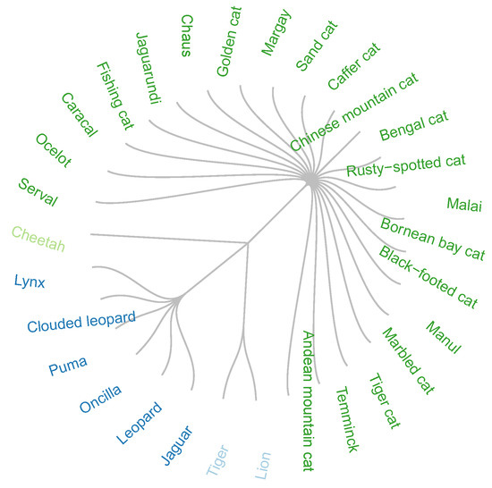
Figure 1. Optimal solution by the Condorcet method.

On the other hand, in the partition into 4 = four groups, applying the k-modes algorithm, it is observed that certain species belong to more than one group and that it does not agree with the classification recognized by zoologists (Figure 2).

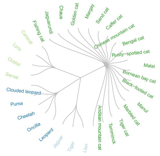
Figure 2. Optimal solution by k-modes, fixing the number of groups at four.

The accuracy of measurement, given in Equation (22), of both solutions given in Figure 1 and Figure 2, is 1 and 0.83, respectively.

$$\mathrm{Accuracy}=\frac{\mathrm{Number}\mathrm{of}\mathrm{correct}\mathrm{predictions}}{\mathrm{Total}\mathrm{number}\mathrm{of}\mathrm{predictions}}.$$

(22)

Next, a comparison was made between the $\alpha$-Condorcet method and the k-modes method for different values of $\alpha$ in order to find the best method that fit the feline data through the within-class inertia index and adjustment rate given in Equations (13) and (21) respectively.

Figure 3, contrasts the quality of groupings by means of the adjustment rate. Therefore, it is observed that the $\alpha$-Condorcet method presents a better quality of partition than the k-modes method for different values of $\alpha$.

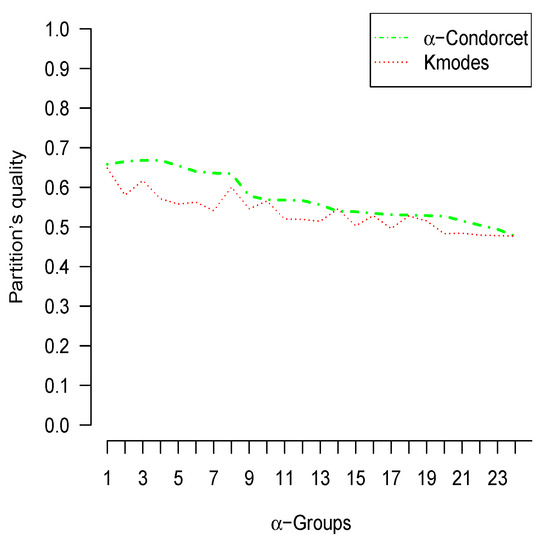
Figure 3. The partitioning quality of feline data under both k-modes and $\alpha$-Condorcet methods.

Figure 4, contrasts the quality of clustering fit through inertia, in the same dataset. In this figure, it is concluded that the intra–class inertia is almost the same for both methods with different values of $\alpha$.

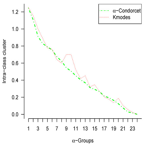
Figure 4. The optimal solution minimizing within-cluster sum-of-squares under both k-modes and $\alpha$-Condorcet methods.

We now use the 1990 US Census dataset to compare the heuristic with k-modes algorithm. This dataset contains a 1% sample of the public use microdata sample person records drawn from the full 1990 census sample. For further references, see https://archive.ics.uci.edu/ml/datasets/US+Census+Data+%281990%29 (accessed on 20 December 2021). The comparisons between both methods were made with 50, 100, 150, and 200 observations.

Table 6 shows that the inertia index is almost the same for both algorithms. However, we observe that the heuristic algorithm is better than k-modes algorithm from the point of view of the quality index.

Table 6. Comparison between k-modes and heuristic algorithm for different sample sizes of the US Census 1990 dataset with $\alpha =4,5,6,7,8$.

	Data Size	$\mathit{\alpha }$	Quality Index	Inertia Index
k-modes	50	4	0.57	3.95
		5	0.56	3.86
		6	0.54	3.66
		7	0.52	3.82
		8	0.54	2.91
Heuristic algorithm		4	0.61	3.49
		5	0.60	3.32
		6	0.58	3.22
		7	0.57	3.10
		8	0.56	3.03
k-modes	100	4	0.58	5.39
		5	0.57	5.08
		6	0.55	4.87
		7	0.53	4.77
		8	0.51	4.80
Heuristic algorithm		4	0.60	4.63
		5	0.60	4.54
		6	0.59	4.45
		7	0.59	4.37
		8	0.58	4.34
k-modes	150	4	0.53	6.04
		5	0.52	5.97
		6	0.52	6.09
		7	0.53	6.06
		8	0.53	5.84
Heuristic algorithm		4	0.60	5.71
		5	0.60	5.65
		6	0.59	5.57
		7	0.59	5.52
		8	0.58	5.44
k-modes	200	4	0.54	6.97
		5	0.52	6.88
		6	0.53	6.82
		7	0.51	6.76
		8	0.51	6.70
Heuristic algorithm		4	0.59	6.89
		5	0.59	6.81
		6	0.59	6.75
		7	0.58	6.70
		8	0.58	6.60

7. Conclusions

In clustering categorical data, many researchers have succeeded in developing unsupervised classification methods without fixing the number of classes a priori. Fixing the number of clusters beforehand, may be major drawback.

However, sometimes it is convenient to identify beforehand the number of groups, as, for instance, in psychometrics. Several methods have been proposed with a known number of clusters. We believe, however, that these methods do not always provide optimal solutions. For this reason, we proposed a new method with a fixed number of groups. This new approach is an extension of the Condorcet method. Although, the exact algorithm of this new approach gives an optimal solution, it consumes too much time. Hence, the heuristic algorithm was introduced. Table 5 shows that the proposed algorithm produces almost the same values of quality and inertia indexes as the exact algorithm.

Next, comparing our approach with k-modes for the feline data, we found that the accuracy index gave better result for the heuristic algorithm. In this case, the comparison was made with the precision index because we know a priori that the number clusters, $\alpha$, is 4. This comparison was also made with the US Census 1990 data, using both partition quality and intra-class inertia indexes. The results in Table 6 show that both methods have almost the same inertia. However, the heuristic algorithm shows an improvement over k-modes in terms of partition quality. Consequently, the following may be concluded:

• We proposed a heuristic algorithm as an alternative algorithm to the exact one. This gives the same or an approximate solution as the exact one.
• From the simulations presented in Table 5, we can conclude that the heuristic algorithm is faster than the exact algorithm.
• The heuristic algorithm produces similar (or even better) results to k-modes.
• We conclude that $\alpha$-Condorcet is a valid technical competitor with respect to the k-modes clustering technique.

References

- Czekanowski, J. Zur Differentialdiagnose der Neandertalgruppe. Korespondentblatt der Deutschen Gesellschaft für Anthropologie Ethnologie und Urgeschichte 1909, XL, 44–47. [Google Scholar]
- Harkanth, S.; Phulpagar, B.D. A survey on clustering methods and algorithms. Int. J. Comput. Sci. Inf. Technol. 2013, 4, 687–691. [Google Scholar]
- Madhulatha, T.S. An overview on clustering methods. arXiv 2012, arXiv:1205.1117. [Google Scholar] [CrossRef]
- Madhulatha, T.S. An overview of clustering methods. Intell. Data Anal. 2007, 11, 583–605. [Google Scholar] [CrossRef]
- Xu, R.; Wunsch, D. Survey of clustering algorithms. IEEE Trans. Neural Netw. 2005, 16, 645–678. [Google Scholar] [CrossRef] [PubMed]
- Xu, D.; Tian, Y. A comprehensive survey of clustering algorithms. Ann. Data Sci. 2015, 2, 165–193. [Google Scholar] [CrossRef]
- Ahlquist, J.S.; Breunig, C. Model-based clustering and typologies in the social sciences. Political Anal. 2010, 20, 325–346. [Google Scholar] [CrossRef]
- Aldenderfer, M.S.; Blashfield, R.K. A review of clustering methods. Clust. Anal. 1984, 33–61. [Google Scholar] [CrossRef]
- Díaz-Costa, E.; Fernández-Cano, A.; Faouzi, T.; Henríquez, C.F. Validación del constructo subyacente en una escala de evaluación del impacto de la investigación educativa sobre la práctica docente mediante análisis factorial confirmatorio. Rev. Investig. Educ. 2015, 33, 47–63. [Google Scholar] [CrossRef]
- Díaz-Costa, E.; Fernández-Cano, A.; Faouzi-Nadim, T.; Caamaño-Carrillo, C. Modelamiento y estimación del índice de impacto de la investigación sobre la docencia. Revista Electrónica Interuniversitaria de Formación del Profesorado 2019, 22, 211–228. [Google Scholar]
- Fonseca, J.R.S. Clustering in the field of social sciences: That is your choice. Int. J. Soc. Res. Methodol. 2013, 16, 403–428. [Google Scholar] [CrossRef]
- Rice, P.M.; Saffer, M.E. Cluster analysis of mixed-level data: Pottery provenience as an example. J. Archaeol. Sci. 1982, 9, 395–409. [Google Scholar] [CrossRef]
- Huang, Z. Extensions to the k-means algorithm for clustering large data sets with categorical values. Data Min. Knowl. Discov. 1998, 2, 283–304. [Google Scholar] [CrossRef]
- Marcotorchino, F.; Michaud, P. Agregation de similarites en classification automatique. Rev. Stat. Appl. 1982, 30, 21–44. [Google Scholar]
- Bock, H.-H. Origins and extensions of the k-means algorithm in cluster analysis. Electron. J. Hist. Probab. Stat. 2008, 4, 1–18. [Google Scholar]
- Forgy, E.W. Cluster analysis of multivariate data: Efficiency versus interpretability of classifications. Biometrics 1965, 21, 768–769. [Google Scholar]
- Jain, A.K. Data clustering: 50 years beyond K-means. IEEE Pattern Recognit. Lett. 2010, 31, 651–666. [Google Scholar] [CrossRef]
- MacQueen, J. Some methods for classification and analysis of multivariate observations. In Proceedings of the Fifth Berkeley Symposium on Mathematical Statistics and Probability; University of California Press: Oakland, CA, USA, 1967; Volume 281–297. [Google Scholar]
- Goyal, M.; Aggarwal, S. A Review on K-Mode Clustering Algorithm. Int. J. Adv. Res. Comput. Sci. 2017, 8, 1615–1620. [Google Scholar] [CrossRef]
- Xiong, T.; Wang, S.; Mayers, A.; Monga, E. DHCC: Divisive hierarchical clustering of categorical data. Data Min. Knowl. Discov. 2012, 24, 103–135. [Google Scholar] [CrossRef]
- Lakshmi, K.; Visalakshi, N.K.; Shanthi, S.; Parvathavarthini, S. Clustering categorical data using K-Modes based on cuckoo searsh optimization algorithm. ICTACT J. Soft Comput. 2017, 8, 1561–1566. [Google Scholar] [CrossRef]
- Dorman, K.S.; Maitra, R. An Efficient k-modes Algorithm for Clustering Categorical Datasets. Stat. Anal. Data Min. ASA Data Sci. J. 2022, 15, 83–97. [Google Scholar] [CrossRef]
- Ali, D.S.; Ghoneim, A.; Saleh, M. K-modes and Entropy Cluster Centers Initialization Methods. In ICORES; SciTePress: Setúbal, Portugal, 2017; pp. 447–454. [Google Scholar]
- Khan, S.S.; Kant, S. Computation of Initial Modes for K-modes Clustering Algorithm Using Evidence Accumulation. In IJCAI; Morgan Kaufmann Publishers: San Francisco, CA, USA, 2007; pp. 2784–2789. [Google Scholar]
- Huang, Z.; Ng, M.K. A fuzzy k-modes algorithm for clustering categorical data. IEEE Trans. Fuzzy Syst. 1999, 7, 446–452. [Google Scholar] [CrossRef]
- Gan, G.; Ma, C.; Wu, J. Data Clustering: Theory, Algorithms, and Applications; Society for Industrial and Applied Mathematics: Philadelphia, PA, USA, 2020. [Google Scholar]
- Jiang, Z.; Liu, X. A novel consensus fuzzy k-modes clustering using coupling DNA-chain-hypergraph P system for categorical data. Processes 2020, 8, 1326. [Google Scholar] [CrossRef]
- Kim, D.-W.; Lee, K.H.; Lee, D. Fuzzy clustering of categorical data using fuzzy centroids. Pattern Recognit. Lett. 2004, 25, 1263–1271. [Google Scholar] [CrossRef]
- Ng, M.K.; Li, M.J.; Huang, J.Z.; He, Z. On the impact of dissimilarity measure in k-modes clustering algorithm. IEEE Trans. Pattern Anal. Mach. Intell. 2007, 29, 503–507. [Google Scholar] [CrossRef] [PubMed]
- Cao, F.; Liang, J.; Li, D.; Bai, L.; Dang, C. A dissimilarity measure for the k-modes clustering algorithm. Knowl.-Based Syst. 2012, 26, 120–127. [Google Scholar] [CrossRef]
- Hazarika, I.; Mahanta, A.K.; Das, D. A New Categorical Data Clustering Technique Based on Genetic Algorithm. Int. J. Appl. Eng. Res. 2017, 12, 12075–12082. [Google Scholar]
- Khandelwal, G.; Sharma, R. A simple yet fast clustering approach for categorical data. Processes 2015, 120, 25–30. [Google Scholar] [CrossRef]
- Seman, A.; Bakar, Z.A.; Sapawi, A.M.; Othman, I.R. A medoid-based method for clustering categorical data. J. Artif. Intell. 2013, 6, 257. [Google Scholar] [CrossRef]
- Michaud, P.; Marcotorchino, F. Modèles d’optimisation en analyse des données relationnelles. Math. Sci. Hum. 1979, 67, 7–38. [Google Scholar]
- Michaud, P. Condorcet: A man of the avant–garde. Appl. Stoch. Model. Data Anal. 1987, 3, 173–189. [Google Scholar] [CrossRef]
- Michaud, P. The true rule of the Marquis de Condorcet. In Compromise, Negotiation and Group Decision; Springer: New York, NY, USA, 1988; pp. 83–100. [Google Scholar]
- Michaud, P. Agrégation à la Majorité II: Analyse du Résultat d’un Vote; Centre Scientifique IBM France: Paris, France, 1985. [Google Scholar]
- Hägele, G.; Pukelsheim, F. Llul’s writings on electoral systems. Stud. Lul. 2001, 41, 3–38. [Google Scholar]
- Marcotorchino, F. Liaison Analyse Factorielle-Analyse Relationnelle: Dualité Burt-Condorcet; IEEE Centre Scientifique IBM France: Paris, France, 1989. [Google Scholar]
- Lebbah, M.; Bennani, Y.; Grozavu, N.; Benhadda, H. Relational analysis for clustering consensus. Mach. Learn. 2010, 45–59. [Google Scholar] [CrossRef]
Publisher’s Note: MDPI stays neutral with regard to jurisdictional claims in published maps and institutional affiliations. |
© 2022 by the authors. Licensee MDPI, Basel, Switzerland. This article is an open access article distributed under the terms and conditions of the Creative Commons Attribution (CC BY) license (https://creativecommons.org/licenses/by/4.0/).