A New Construction and Convergence Analysis of Non-Monotonic Iterative Methods for Solving ρ-Demicontractive Fixed Point Problems and Variational Inequalities Involving Pseudomonotone Mapping

Abstract

Two new inertial-type extragradient methods are proposed to find a numerical common solution to the variational inequality problem involving a pseudomonotone and Lipschitz continuous operator, as well as the fixed point problem in real Hilbert spaces with a $\rho$-demicontractive mapping. These inertial-type iterative methods use self-adaptive step size rules that do not require previous knowledge of the Lipschitz constant. We also show that the proposed methods strongly converge to a solution of the variational inequality and fixed point problems under appropriate standard test conditions. Finally, we present several numerical examples to show the effectiveness and validation of the proposed methods.

1. Introduction

Assume that $\mathcal{Y}$ is a nonempty, closed, and convex subset of a real Hilbert space $\mathcal{X}$ with the inner product $⟨·,·⟩$ and the induced norm $\parallel ·\parallel .$ The main contribution of this study is to investigate the convergence analysis of the iterative schemes for solving variational inequality and fixed point problems in real Hilbert spaces. The reason and inspiration for investigating such a common solution problem is its potential applicability to mathematical models whose constraints can be stated as fixed point problems. This is especially relevant in applications such as signal processing, composite minimization, optimum control, and image restoration; see, for example, [1,2,3,4,5]. Let us take a look at both of the problems highlighted by this research.

Let $\Im :\mathcal{Y}\to \mathcal{X}$ be an operator. First, we look at the classic variational inequality problem [6,7] which is expressed as follows:

$$\mathrm{Find}{r}^{*}\in \mathcal{Y}\mathrm{such}\mathrm{that}⟨\Im \left(r^{*}\right),y-r^{*}⟩\ge 0,\forall y\in \mathcal{Y}.$$

(1)

The solution set of a problem (1) is denoted by $VI(\mathcal{Y},\Im ).$ The variational inequality problem has been widely applied to study real world applications, such as partial differential equations, optimization, optimal control, mechanics, mathematical programming, and finance (see [8,9,10,11,12,13,14]). The problem (1) is a significant one in applied sciences. Many authors have committed themselves to investigating not only the theory of existence and the stability of solutions, but also iterative methods for solving such problems.

On the other hand, projection methods are important for determining the numerical solution to variational inequalities. Several authors proposed various projection methods to solve the problem (1) (see for details [15,16,17,18,19,20,21,22,23,24,25,26,27,28,29,30,31,32]). Most methods for solving the problem (1) use the projection method, which is computed on the feasible set $\mathcal{Y}.$ Korpelevich [15] and Antipin [33] established the extragradient method described below. Their method takes the following form:

$$\left\{\begin{array}{c}{u}_1\in \mathcal{Y},\hfill \\ y_k=P_{\mathcal{Y}}[u_k-\gimel \Im \left(u_k\right)],\hfill \\ u_{k+1}=P_{\mathcal{Y}}[u_k-\gimel \Im \left(y_k\right)],\hfill \end{array}\right.$$

(2)

where $0<\gimel <\frac{1}{L}.$ According to the above method, each iteration must estimate two projections on the feasible set $\mathcal{Y}.$ Of course, if the feasible set $\mathcal{Y}$ has a convoluted structure, this might have an impact on the computing efficacy of the approach adopted. In this part, we will limit our attention to giving various approaches for overcoming this obstacle. The first is the following subgradient extragradient method proposed by Censor et al. [17]. This method is in the following form:

$$\left\{\begin{array}{c}{u}_1\in \mathcal{Y},\hfill \\ y_k=P_{\mathcal{Y}}[u_k-\gimel \Im \left(u_k\right)],\hfill \\ u_{k+1}=P_{{\mathcal{X}}_k}[u_k-\gimel \Im \left(y_k\right)],\hfill \end{array}\right.$$

(3)

where $0<\gimel <\frac{1}{L}$ and

$${\mathcal{X}}_k=\{z\in \mathcal{X}:⟨u_k-\gimel \Im \left(u_k\right)-y_k,z-y_k⟩\le 0\}.$$

Furthermore, Tseng’s extragradient method [19] requires only one projection for each iteration. This method is written as follows:

$$\left\{\begin{array}{c}{u}_1\in \mathcal{Y},\hfill \\ y_k=P_{\mathcal{Y}}[u_k-\gimel \Im \left(u_k\right)],\hfill \\ u_{k+1}=y_k-\gimel \left[\Im \left(y_k\right)-\Im \left(u_k\right)\right].\hfill \end{array}\right.$$

(4)

where $0<\gimel <\frac{1}{L}.$ In terms of computation, the method (4) is extremely efficient because it only requires one solution to a minimization problem per iteration. As a result, the method (4) is less computationally expensive and performs better in most situations.

Let $\mathcal{T}:\mathcal{X}\to \mathcal{X}$ be a mapping and the fixed point problem (FPP) for the mapping $\mathcal{T}$ is to: find $r^{*}\in \mathcal{X}$ such that

$$\mathcal{T}\left(r^{*}\right)=r^{*}.$$

(5)

The solution set of a fixed point problem is known as the fixed point set of a mapping $\mathcal{T}$ and is denoted by $Fix\left(\mathcal{T}\right).$ Most of methods for solving the problem (5) are derived from the standard Mann iteration, specifically, from $u_1\in \mathcal{X}$ and construct sequence $\left\{u_{k+1}\right\}$ for all $k\ge 1$ by

$$u_{k+1}={\alpha }_k{u}_k+(1-{\alpha }_k)\mathcal{T}{u}_k,$$

(6)

where the variable sequence $\left\{{\alpha }_k\right\}$ must meet certain requirements in order to accomplish weak convergence. Another formalised iterative approach that is more effective in infinite-dimensional Hilbert spaces for achieving strong convergence is the Halpern iteration. The iterative sequence can be written as follows:

$$u_{k+1}={\alpha }_k{u}_1+(1-{\alpha }_k)\mathcal{T}{u}_k,$$

(7)

where $u_1\in \mathcal{X}$ and the sequence ${\alpha }_k\subset (0,1)$ is non-summable and slowly diminishing, i.e.,

$${\alpha }_k\to 0\mathit{and}\sum _{k=1}^{+\infty }{\alpha }_k=+\infty .$$

Furthermore, it is worth mentioning that, in addition to the Halpern iteration, there is a general form of it, namely the viscosity method [20], in which the cost mapping $\mathcal{T}$ is merged with a contraction mapping in the iterates. Finally, another technique that provides strong convergence is the hybrid steepest descent method proposed in [34].

Tan et al. [35,36] recently introduced a new numerical method, namely the extragradient viscosity method, for solving variational inequalities involving a constraint set as a fixed point set for a $\rho$-demicontractive mapping. These methods were obtained by combining the extragradient methods [15,17] with the Mann-type method [37] and the viscosity-type method [20]. The authors proved that all methods have strong convergence when the operator is pseudomonotone and meets the Lipschitz criterion. These methods have the advantage of being numerically computed using optimization tools, as discussed in [35,36].

The primary disadvantage of these methods is that they rely on viscosity and Mann-type techniques to obtain strong convergence. As we all know, achieving strong convergence is critical for iterative sequences, especially in infinite-dimensional spaces. There are only a few techniques with strong convergence that use inertial schemes. The Mann and Viscosity types of steps may be difficult to estimate from an algorithmic perspective, affecting the algorithm’s convergence rate and applicability. These methods increase the number of numerical and computational steps, making the system more complex.

Hence, a natural question arises:

Is it possible to introduce strongly convergent inertial extragradient methods for solving variational inequalities and fixed point problems with a self-adaptive step size rule without requiring Mann and Viscosity-type methods?

Motivated by the above, as well as the works cited in [35,36], we provide the positive answer to the above question by introducing two strong convergence extragradient-type methods for solving pseudomonotone variational inequalities and the $\rho$-demicontractive fixed point problem in real Hilbert spaces. Furthermore, we avoid the use of any hybrid schemes, such as the Mann-type and the Viscosity scheme, in order to obtain the strong convergence of these methods. We proposed novel methods that leverage inertial schemes and have a strong convergence.

The paper is organized as follows: Section 2 contains basic results and identities. Section 3 introduces two novel methods and proves their convergence analysis. Finally, Section 4 provides some numerical data to explain the practical efficacy of the proposed methods.

2. Preliminaries

Let $\mathcal{Y}$ be a nonempty, closed, and convex subset of $\mathcal{X},$ the real Hilbert space. Assume that the sequences $u_k\rightharpoonup u$ and $u_k\to u$ represent the weak and strong convergence of $u_k$ to $u.$ For each $u,y\in \mathcal{X},$ the following information is available to us:

(1)

${\parallel u+y\parallel }^2={\parallel u\parallel }^2+2⟨u,y⟩+{\parallel y\parallel }^2;$

(2)

${\parallel u+y\parallel }^2\le {\parallel u\parallel }^2+2⟨y,u+y⟩;$

(3)

${\parallel bu+(1-b)y\parallel }^2={b\parallel u\parallel }^2+{(1-b)\parallel y\parallel }^2-b(1-b){\parallel u-y\parallel }^2.$

The definition of metric projection $P_{\mathcal{Y}}\left(u\right)$ of $u\in \mathcal{X}$ is defined by

$$P_{\mathcal{Y}}\left(u\right)=\underset{}{argmin}\{\parallel u-y\parallel :y\in \mathcal{Y}\}.$$

It is well-known that $P_{\mathcal{Y}}$ is non-expansive and $P_{\mathcal{Y}}$ satisfies the following conditions:

(1)

$⟨u-P_{\mathcal{Y}}\left(u\right),y-P_{\mathcal{Y}}\left(u\right)⟩\le 0,\forall y\in \mathcal{Y};$

(2)

$\parallel P_{\mathcal{Y}}\left(u\right)-P_{\mathcal{Y}}{\left(y\right)\parallel }^2\le ⟨P_{\mathcal{Y}}\left(u\right)-P_{\mathcal{Y}}\left(y\right),u-y⟩,\forall y\in \mathcal{Y}.$

Definition  1.

In [38] suppose that $\mathcal{T}:\mathcal{X}\to \mathcal{X}$ is a nonlinear function with $Fix\left(\mathcal{T}\right)\ne \varnothing .$ Then, $I-\mathcal{T}$ is said to be demiclosed at zero if, for all $\left\{u_k\right\}$ in $\mathcal{X},$ the following conclusion holds:

$$u_k\rightharpoonup u\mathit{and}(I-\mathcal{T})u_k\to 0\Rightarrow u\in Fix\left(\mathcal{T}\right).$$

Lemma  1.

In [39] let $\left\{p_k\right\}\subset [0,+\infty ),$ $\left\{q_k\right\}\subset (0,1)$ and $\left\{r_k\right\}\subset \mathbb{R}$ are three sequences meet the following requirements:

$$p_{k+1}\le (1-q_k)p_k+q_k{r}_k,\forall k\in \mathbb{N}\mathit{and}\sum _{k=1}^{+\infty }{q}_k=+\infty .$$

If ${lim\; sup}_{j\to +\infty }{r}_{k_j}\le 0$ for each subsequence $\left\{p_{k_j}\right\}$ of $\left\{p_j\right\}$ meet

$$\underset{j\to +\infty }{lim\; inf}(p_{k_j+1}-p_{k_j})\ge 0.$$

Then, ${lim}_{k\to +\infty }{p}_k=0.$

Definition 2.

In [40,41] for any $u_1,u_2\in \mathcal{X};$ $p\in Fix\left(\mathcal{T}\right),$ an operator $\mathcal{T}:\mathcal{X}\to \mathcal{X}$ is said to be

(1)

L-Lipschitz continuous if there exists a constant $L>0$ such that

$$\parallel \Im \left(u_1\right)-\Im \left(u_2\right)\parallel \le L\parallel u_1-u_2\parallel ;$$

(2)

pseudomonotone if

$$⟨\Im \left(u_1\right),u_2-u_1⟩\ge 0⟹⟨\Im \left(u_2\right),u_1-u_2⟩\le 0;$$

(3)

sequentially weakly continuous if a sequence $\{\Im \left(u_k\right)\}$ weakly convergent to $\Im \left(u\right)$ for any sequence $\left\{u_k\right\}$ that is weakly convergent to $u;$

(4)

ρ-demicontractive if there exists a constant $0\le \rho <1$ such that

$$\parallel \mathcal{T}\left(u_1\right){-p\parallel }^2\le \parallel u_1{-p\parallel }^2+\rho {\parallel (I-\mathcal{T})\left(u_1\right)\parallel }^2,$$

or equivalently

$$⟨\mathcal{T}\left(u_1\right)-u_1,u_1-p⟩\le \frac{\rho -1}{2}{\parallel u_1-\mathcal{T}\left(u_1\right)\parallel }^2.$$

Next, in order to prove the strong convergence theorems, we assumed the following conditions are satisfied:

(ℑ 1)

The solution set $Fix\left(\mathcal{T}\right)\cap VI(\mathcal{Y},\Im )\ne \varnothing ;$

(ℑ 2)

The mapping ℑ is pseudomonotone, Lipschitz continuous and sequentially weakly continuous;

(ℑ 3)

The $\mathcal{T}:\mathcal{X}\to \mathcal{X}$ is $\rho$-demicontractive and $(I-\mathcal{T})$ is demiclosed at zero.

3. Main Results

In this section, we examine at the convergence of two new inertial extragradient methods for solving variational inequality and fixed point problems in detail. These techniques made use of fixed and non-monotone step size criteria.

Lemma  2.

A sequence $\left\{{\gimel }_k\right\}$ generated by (15) is convergent to ℷ and bounded by $min\left\{\frac{\mu }{L},{\gimel }_1\right\}\le \gimel \le {\gimel }_1+P$, where ${\displaystyle P=\sum _{k=1}^{+\infty }{\varkappa }_k}$.

Proof. 

Since the mapping ℑ is Lipschitz continuous, there exists a positive constant $L.$ It is given that $⟨\Im \left(t_k\right)-\Im \left(y_k\right),z_k-y_k⟩>0,$ and

$$\begin{array}{cc}\hfill \frac{\mu (\parallel t_k-y_k{\parallel }^2+\parallel z_k-y_k{\parallel }^2)}{2⟨\Im \left(t_k\right)-\Im \left(y_k\right),z_k-y_k⟩}& \ge \frac{2\mu \parallel t_k-y_k\parallel \parallel z_k-y_k\parallel }{2\parallel \Im \left(t_k\right)-\Im \left(y_k\right)\parallel \parallel z_k-y_k\parallel }\hfill \\ \hfill & \ge \frac{2\mu \parallel t_k-y_k\parallel \parallel z_k-y_k\parallel }{2L\parallel t_k-y_k\parallel \parallel z_k-y_k\parallel }\ge \frac{\mu }{L}.\hfill \end{array}$$

(8)

Using mathematical induction on the definition of ${\gimel }_{k+1},$ we have

$$min\left\{\frac{\mu }{L},{\gimel }_1\right\}\le {\gimel }_k\le {\gimel }_1+P.$$

Let ${[{\gimel }_{k+1}-{\gimel }_k]}^{+}=max\left\{0,{\gimel }_{k+1}-{\gimel }_k\right\}$ and ${[{\gimel }_{k+1}-{\gimel }_k]}^{-}=max\left\{0,-({\gimel }_{k+1}-{\gimel }_k)\right\}.$ From the definition of $\left\{{\gimel }_k\right\}$, we have

$$\sum _{k=1}^{+\infty }{({\gimel }_{k+1}-{\gimel }_k)}^{+}=\sum _{k=1}^{+\infty }max\left\{0,{\gimel }_{k+1}-{\gimel }_k\right\}\le P<+\infty .$$

(9)

That is, the series ${\displaystyle \sum _{k=1}^{+\infty }{({\gimel }_{k+1}-{\gimel }_k)}^{+}}$ is convergent. Next, we need to prove the convergence of ${\displaystyle \sum _{k=1}^{+\infty }{({\gimel }_{k+1}-{\gimel }_k)}^{-}.}$ Let ${\displaystyle \sum _{k=1}^{+\infty }{({\gimel }_{k+1}-{\gimel }_k)}^{-}=+\infty }$. For this reason, we have ${\gimel }_{k+1}-{\gimel }_k={({\gimel }_{k+1}-{\gimel }_k)}^{+}-{({\gimel }_{k+1}-{\gimel }_k)}^{-}.$ Thus, we obtain

$${\displaystyle {\gimel }_{k+1}-{\gimel }_1=\sum _{k=0}^k({\gimel }_{k+1}-{\gimel }_k)=\sum _{k=0}^k{({\gimel }_{k+1}-{\gimel }_k)}^{+}-\sum _{k=0}^k{({\gimel }_{k+1}-{\gimel }_k)}^{-}.}$$

(10)

By letting $k\to +\infty$ in expression (10), we have ${\gimel }_k\to -\infty$ as $k\to +\infty .$ This is a contradiction. Due to the convergence of the series ${\displaystyle \sum _{k=0}^k{({\gimel }_{k+1}-{\gimel }_k)}^{+}}$ and ${\displaystyle \sum _{k=0}^k{({\gimel }_{k+1}-{\gimel }_k)}^{-}}$ taking $k\to +\infty$ in expression (10), we obtain ${lim}_{k\to +\infty }{\gimel }_k={\gimel }_{.}$ This completes the proof of lemma.    □

Lemma  3.

The step size sequence $\left\{{\gimel }_k\right\}$ generated in (24) is monotonically decreasing and bounded by $min\left\{\frac{\mu }{L},{\gimel }_1\right\}\le \gimel \le {\gimel }_1+P,$ where ${\displaystyle P=\sum _{k=1}^{+\infty }{\varkappa }_k.}$

Proof. 

It is given that ℑ is Lipschitz-continuous with constant $L>0,$ and we have

$$\begin{array}{cc}\hfill \frac{\mu \parallel t_k-y_k\parallel }{\parallel \Im \left(t_k\right)-\Im \left(y_k\right)\parallel }& \ge \frac{\mu \parallel t_k-y_k\parallel }{L\parallel t_k-y_k\parallel }\ge \frac{\mu }{L}.\hfill \end{array}$$

(11)

Using mathematical induction on the definition of ${\gimel }_{k+1},$ we have

$$min\left\{\frac{\mu }{L},{\gimel }_1\right\}\le {\gimel }_k\le {\gimel }_1+P.$$

Let ${[{\gimel }_{k+1}-{\gimel }_k]}^{+}=max\left\{0,{\gimel }_{k+1}-{\gimel }_k\right\}$ and ${[{\gimel }_{k+1}-{\gimel }_k]}^{-}=max\left\{0,-({\gimel }_{k+1}-{\gimel }_k)\right\}.$ From the definition of $\left\{{\gimel }_k\right\}$, we have

$$\sum _{k=1}^{+\infty }{({\gimel }_{k+1}-{\gimel }_k)}^{+}=\sum _{k=1}^{+\infty }max\left\{0,{\gimel }_{k+1}-{\gimel }_k\right\}\le P<+\infty .$$

(12)

That is, the series ${\displaystyle \sum _{k=1}^{+\infty }{({\gimel }_{k+1}-{\gimel }_k)}^{+}}$ is convergent. Next, we need to prove the convergence of ${\displaystyle \sum _{k=1}^{+\infty }{({\gimel }_{k+1}-{\gimel }_k)}^{-}.}$ Let ${\displaystyle \sum _{k=1}^{+\infty }{({\gimel }_{k+1}-{\gimel }_k)}^{-}=+\infty }$. For this reason, we have ${\gimel }_{k+1}-{\gimel }_k={({\gimel }_{k+1}-{\gimel }_k)}^{+}-{({\gimel }_{k+1}-{\gimel }_k)}^{-}.$ Thus, we obtain

$${\displaystyle {\gimel }_{k+1}-{\gimel }_1=\sum _{k=0}^k({\gimel }_{k+1}-{\gimel }_k)=\sum _{k=0}^k{({\gimel }_{k+1}-{\gimel }_k)}^{+}-\sum _{k=0}^k{({\gimel }_{k+1}-{\gimel }_k)}^{-}.}$$

(13)

By letting $k\to +\infty$ in expression (13), we have ${\gimel }_k\to -\infty$ as $k\to +\infty .$ This is a contradiction. Due to the convergence of the series ${\displaystyle \sum _{k=0}^k{({\gimel }_{k+1}-{\gimel }_k)}^{+}}$ and ${\displaystyle \sum _{k=0}^k{({\gimel }_{k+1}-{\gimel }_k)}^{-}}$ taking $k\to +\infty$ in (13), we obtain ${lim}_{k\to +\infty }{\gimel }_k={\gimel }_{.}$ This completes the proof of lemma.    □

Lemma  4.

Let $\Im :\mathcal{X}\to \mathcal{X}$ be a mapping satisfies the conditions(ℑ 1)– (ℑ 2). Let $\left\{u_k\right\}$ be a sequence is generated by Algorithm 1. For each $r^{*}\in VI(\mathcal{Y},\Im ),$ we have

$$\parallel z_k-r^{*}{\parallel }^2\le \parallel t_k-r^{*}{\parallel }^2-\left(1-\frac{\mu {\gimel }_k}{{\gimel }_{k+1}}\right)\parallel t_k-y_k{\parallel }^2-\left(1-\frac{\mu {\gimel }_k}{{\gimel }_{k+1}}\right){\parallel z_k-y_k\parallel }^2.$$

Algorithm 1 Inertial Subgradient Extragradient Method with Non-Monotone Step Size Rule.

Step 0: Take $u_0,u_1\in \mathcal{Y},$ $\theta \in (0,1),$ $\mu \in (0,1),$ ${\gimel }_1>0.$ Moreover, select a non-negative real sequence $\left\{{\varkappa }_k\right\}$ such that ${\sum }_{k=1}^{+\infty }{\varkappa }_k<+\infty$ and $\left\{{\beta }_k\right\}\subset (0,1)$ satisfies the following conditions: $$\underset{k\to +\infty }{lim}{\beta }_k=0\mathrm{and}\sum _{k=1}^{+\infty }{\beta }_k=+\infty .$$ Step 1: Compute $$t_k=u_k+{\theta }_k(u_k-u_{k-1})-{\beta }_k\left[u_k+{\theta }_k(u_k-u_{k-1})\right],$$ while ${\theta }_k$ taken as follows: $$0\le {\theta }_k\le \widehat{{\theta }_k}\mathrm{and}\widehat{{\theta }_k}=\left\{\begin{array}{cc}min\left\{\frac{\theta }{2},\frac{{ϵ}_k}{\parallel u_k-u_{k-1}\parallel }\right\}\hfill & \mathrm{if}{u}_k\ne u_{k-1},\hfill \\ \frac{\theta }{2}& \mathrm{otherwise}.\end{array}\right.$$ (14) Moreover, a positive sequence ${ϵ}_k=\circ \left({\beta }_k\right)$ such that ${lim}_{k\to +\infty }\frac{{ϵ}_k}{{\beta }_k}=0.$ Step 2: Compute $$y_k=P_{\mathcal{Y}}(t_k-{\gimel }_k\Im \left(t_k\right)).$$ If $t_k=y_k$, then STOP. Else, move to Step 3. Step 3: First, construct a half-space ${\mathcal{X}}_k=\{z\in \mathcal{X}:⟨t_k-{\gimel }_k\Im \left(t_k\right)-y_k,z-y_k⟩\le 0\}$ and compute $$z_k=P_{{\mathcal{X}}_k}(t_k-{\gimel }_k\Im \left(y_k\right)).$$ Step 4: Compute $u_{k+1}=(1-{\alpha }_k)z_k+{\alpha }_k\mathcal{T}\left(z_k\right).$ Step 5: Compute $${\gimel }_{k+1}=\left\{\begin{array}{c}min\left\{{\gimel }_k+{\varkappa }_k,\frac{\mu \parallel t_k-y_k{\parallel }^2+\mu {\parallel z_k-y_k\parallel }^2}{2\left[⟨\Im \left(t_k\right)-\Im \left(y_k\right),z_k-y_k⟩\right]}\right\}\mathrm{if}⟨\Im \left(t_k\right)-\Im \left(y_k\right),z_k-y_k⟩>0,\hfill \\ {\gimel }_k+{\varkappa }_k,otherwise.\end{array}\right.$$ (15) Set $k:=k+1$ and go back to Step 1.

Proof. 

First, we have to compute the following

$$\begin{array}{cc}\hfill {∥z_k-r^{*}∥}^2& ={∥P_{{\mathcal{X}}_k}[t_k-{\gimel }_k\Im \left(y_k\right)]-r^{*}∥}^2\hfill \\ \hfill & ={∥P_{{\mathcal{X}}_k}[t_k-{\gimel }_k\Im \left(y_k\right)]+[t_k-{\gimel }_k\Im \left(y_k\right)]-[t_k-{\gimel }_k\Im \left(y_k\right)]-r^{*}∥}^2\hfill \\ \hfill & ={∥[t_k-{\gimel }_k\Im \left(y_k\right)]-r^{*}∥}^2+{∥P_{{\mathcal{X}}_k}[t_k-{\gimel }_k\Im \left(y_k\right)]-[t_k-{\gimel }_k\Im \left(y_k\right)]∥}^2\hfill \\ \hfill & +2⟨P_{{\mathcal{X}}_k}[t_k-{\gimel }_k\Im \left(y_k\right)]-[t_k-{\gimel }_k\Im \left(y_k\right)],[t_k-{\gimel }_k\Im \left(y_k\right)]-r^{*}⟩.\hfill \end{array}$$

(16)

It is hypothesized that $r^{*}\in VI(\mathcal{Y},\Im )\subset \mathcal{Y}\subset {\mathcal{X}}_k.$ Thus, we have

$$\begin{array}{cc}\hfill & {∥P_{{\mathcal{X}}_k}[t_k-{\gimel }_k\Im \left(y_k\right)]-[t_k-{\gimel }_k\Im \left(y_k\right)]∥}^2\hfill \\ \hfill & +⟨P_{{\mathcal{X}}_k}[t_k-{\gimel }_k\Im \left(y_k\right)]-[t_k-{\gimel }_k\Im \left(y_k\right)],[t_k-{\gimel }_k\Im \left(y_k\right)]-r^{*}⟩\hfill \\ \hfill & =⟨[t_k-{\gimel }_k\Im \left(y_k\right)]-P_{{\mathcal{X}}_k}[t_k-{\gimel }_k\Im \left(y_k\right)],r^{*}-P_{{\mathcal{X}}_k}[t_k-{\gimel }_k\Im \left(y_k\right)]⟩\le 0.\hfill \end{array}$$

(17)

It also indicates that

$$\begin{array}{cc}\hfill & ⟨P_{{\mathcal{X}}_k}[t_k-{\gimel }_k\Im \left(y_k\right)]-[t_k-{\gimel }_k\Im \left(y_k\right)],[t_k-{\gimel }_k\Im \left(y_k\right)]-r^{*}⟩\hfill \\ \hfill & \le -{∥P_{{\mathcal{X}}_k}[t_k-{\gimel }_k\Im \left(y_k\right)]-[t_k-{\gimel }_k\Im \left(y_k\right)]∥}^2.\hfill \end{array}$$

(18)

We obtain by combining Equations (16) and (18)

$$\begin{array}{cc}\hfill \parallel z_k-r^{*}{\parallel }^2& \le {∥t_k-{\gimel }_k\Im \left(y_k\right)-r^{*}∥}^2-{∥P_{{\mathcal{X}}_k}[t_k-{\gimel }_k\Im \left(y_k\right)]-[t_k-{\gimel }_k\Im \left(y_k\right)]∥}^2\hfill \\ \hfill & \le \parallel t_k-r^{*}{\parallel }^2-{\parallel t_k-z_k\parallel }^2+2{\gimel }_k⟨\Im \left(y_k\right),r^{*}-z_k⟩.\hfill \end{array}$$

(19)

We acquire ℑ on $\mathcal{Y}$ as a result of the definition of a mapping ℑ on $\mathcal{Y}.$ Thus, we have

$$⟨\Im \left(r^{*}\right),y-r^{*}⟩-⟨\Im \left(y\right),y-r^{*}⟩\le 0,\forall y\in \mathcal{Y}.$$

Since $r^{*}\in VI(\mathcal{Y},\Im ),$ we have

$$⟨\Im \left(y\right),y-r^{*}⟩\ge 0,\forall y\in \mathcal{Y}.$$

By letting $y=y_k\in \mathcal{Y},$ we have

$$⟨\Im \left(y_k\right),y_k-r^{*}⟩\ge 0.$$

Thus, we have

$$⟨\Im \left(y_k\right),r^{*}-z_k⟩=⟨\Im \left(y_k\right),r^{*}-y_k⟩+⟨\Im \left(y_k\right),y_k-z_k⟩\le ⟨\Im \left(y_k\right),y_k-z_k⟩.$$

(20)

We obtain by combining formulas (19) and (20)

$$\begin{array}{cc}\hfill \parallel z_k-r^{*}{\parallel }^2& \le \parallel t_k-r^{*}{\parallel }^2-{\parallel t_k-z_k\parallel }^2+2{\gimel }_k⟨\Im \left(y_k\right),y_k-z_k⟩\hfill \\ \hfill & \le \parallel t_k-r^{*}{\parallel }^2-{\parallel t_k-y_k+y_k-z_k\parallel }^2+2{\gimel }_k⟨\Im \left(y_k\right),y_k-z_k⟩\hfill \\ \hfill & \le \parallel t_k-r^{*}{\parallel }^2-\parallel t_k-y_k{\parallel }^2-{\parallel y_k-z_k\parallel }^2+2⟨t_k-{\gimel }_k\Im \left(y_k\right)-y_k,z_k-y_k⟩.\hfill \end{array}$$

(21)

From given $z_k=P_{{\mathcal{X}}_k}[t_k-{\gimel }_k\Im \left(y_k\right)]$ we have

$$\begin{array}{cc}\hfill 2⟨t_k-{\gimel }_k\Im \left(y_k\right)-y_k,z_k-y_k⟩& =2⟨t_k-{\gimel }_k\Im \left(t_k\right)-y_k,z_k-y_k⟩+2{\gimel }_k⟨\Im \left(t_k\right)-\Im \left(y_k\right),z_k-y_k⟩\hfill \\ \hfill & \le \frac{{\gimel }_k}{{\gimel }_{k+1}}2{\gimel }_{k+1}⟨\Im \left(t_k\right)-\Im \left(y_k\right),z_k-y_k⟩\hfill \\ \hfill & \le \frac{\mu {\gimel }_k}{{\gimel }_{k+1}}\parallel t_k-y_k{\parallel }^2+\frac{\mu {\gimel }_k}{{\gimel }_{k+1}}{\parallel z_k-y_k\parallel }^2.\hfill \end{array}$$

(22)

From (21) and (22) we obtain

$$\begin{array}{cc}\hfill \parallel z_k-r^{*}{\parallel }^2& \le \parallel t_k-r^{*}{\parallel }^2-\parallel t_k-y_k{\parallel }^2-{\parallel y_k-z_k\parallel }^2+\frac{{\gimel }_k}{{\gimel }_{k+1}}\left[\mu \parallel t_k-y_k{\parallel }^2+\mu {\parallel z_k-y_k\parallel }^2\right]\hfill \\ \hfill & \le \parallel t_k-r^{*}{\parallel }^2-\left(1-\frac{\mu {\gimel }_k}{{\gimel }_{k+1}}\right)\parallel t_k-y_k{\parallel }^2-\left(1-\frac{\mu {\gimel }_k}{{\gimel }_{k+1}}\right){\parallel z_k-y_k\parallel }^2.\hfill \end{array}$$

(23)

   □

Lemma  5.

Let $\Im :\mathcal{X}\to \mathcal{X}$ satisfies the items (ℑ 1)– (ℑ 2). Let $\left\{u_k\right\}$ be a sequence is generated by Algorithm 2. Then, for each $r^{*}\in VI(\mathcal{Y},\Im ),$ we have

$$\parallel z_k-r^{*}{\parallel }^2\le {∥t_k-r^{*}∥}^2-\left(1-{\mu }^2\frac{{\gimel }_k^2}{{\gimel }_{k+1}^2}\right){∥t_k-y_k∥}^2.$$

Algorithm 2 Inertial Tseng’s Extragradient Method with Non-Monotone Step Size Rule.

Step 0: Take $u_0,u_1\in \mathcal{Y},$ $\theta \in (0,1),$ $\mu \in (0,1),$ ${\gimel }_1>0.$ Moreover, select a non-negative real sequence $\left\{{\varkappa }_k\right\}$ such that ${\sum }_{k=1}^{+\infty }{\varkappa }_k<+\infty$ and $\left\{{\beta }_k\right\}\subset (0,1)$ satisfies the following conditions: $$\underset{k\to +\infty }{lim}{\beta }_k=0\mathit{and}\sum _{k=1}^{+\infty }{\beta }_k=+\infty .$$ Step 1: Compute $$t_k=u_k+{\theta }_k(u_k-u_{k-1})-{\beta }_k\left[u_k+{\theta }_k(u_k-u_{k-1})\right],$$ while ${\theta }_k$ taken as follows: $$0\le {\theta }_k\le \widehat{{\theta }_k}\mathrm{and}\widehat{{\theta }_k}=\left\{\begin{array}{cc}min\left\{\frac{\theta }{2},\frac{{ϵ}_k}{\parallel u_k-u_{k-1}\parallel }\right\}\hfill & \mathrm{if}{u}_k\ne u_{k-1},\hfill \\ \frac{\theta }{2}& \mathrm{otherwise}.\end{array}\right.$$ (24) Moreover, a positive sequence ${ϵ}_k=\circ \left({\beta }_k\right)$ such that ${lim}_{k\to +\infty }\frac{{ϵ}_k}{{\beta }_k}=0.$ Step 2: Compute $$y_k=P_{\mathcal{Y}}(t_k-{\gimel }_k\Im \left(t_k\right)).$$ If $t_k=y_k$, then STOP. Otherwise, go to Step 3. Step 3: Compute $$z_k=y_k+{\gimel }_k\left[\Im \left(t_k\right)-\Im \left(y_k\right)\right].$$ Step 4: Compute $$u_{k+1}=(1-{\alpha }_k)z_k+{\alpha }_k\mathcal{T}\left(z_k\right).$$ Step 5: Compute $$\left\{\begin{array}{c}min\left\{{\gimel }_k+{\varkappa }_k,\frac{\mu \parallel t_k-y_k\parallel }{\parallel \Im \left(t_k\right)-A\left(y_k\right)\parallel }\right\}\mathrm{if}\Im \left(t_k\right)\ne \Im \left(y_k\right),\hfill \\ {\gimel }_k+{\varkappa }_k,\mathrm{otherwise}.\end{array}\right.$$ (25) Set $k:=k+1$ and move back to Step 1.

Proof. 

From $r^{*}\in VI(\mathcal{Y},\Im )$ and due to value of $z_k,$ we may write

$$\begin{array}{cc}\hfill & {∥z_k-r^{*}∥}^2\hfill \\ \hfill & ={∥y_k+{\gimel }_k[\Im \left(u_k\right)-\Im \left(y_k\right)]-r^{*}∥}^2\hfill \\ \hfill & ={∥y_k-r^{*}∥}^2+{\gimel }_k^2{∥\Im \left(u_k\right)-\Im \left(y_k\right)∥}^2+2{\gimel }_k⟨y_k-r^{*},\Im \left(u_k\right)-\Im \left(y_k\right)⟩\hfill \\ \hfill & ={∥y_k+u_k-u_k-r^{*}∥}^2+{\gimel }_k^2{∥\Im \left(u_k\right)-\Im \left(y_k\right)∥}^2+2{\gimel }_k⟨y_k-r^{*},\Im \left(u_k\right)-\Im \left(y_k\right)⟩\hfill \\ \hfill & ={∥y_k-u_k∥}^2+{∥u_k-r^{*}∥}^2+2⟨y_k-u_k,u_k-r^{*}⟩\hfill \\ \hfill & +{\gimel }_k^2{∥\Im \left(u_k\right)-\Im \left(y_k\right)∥}^2+2{\gimel }_k⟨y_k-r^{*},\Im \left(u_k\right)-\Im \left(y_k\right)⟩\hfill \\ \hfill & ={∥u_k-r^{*}∥}^2+{∥y_k-u_k∥}^2+2⟨y_k-u_k,y_k-r^{*}⟩+2⟨y_k-u_k,u_k-y_k⟩\hfill \\ \hfill & +{\gimel }_k^2{∥\Im \left(u_k\right)-\Im \left(y_k\right)∥}^2+2{\gimel }_k⟨y_k-r^{*},\Im \left(u_k\right)-\Im \left(y_k\right)⟩.\hfill \end{array}$$

(26)

Due to the value of $y_k=P_{\mathcal{Y}}[u_k-{\gimel }_k\Im \left(u_k\right)]$ we have

$$⟨u_k-{\gimel }_k\Im \left(u_k\right)-y_k,y-y_k⟩\le 0,\forall y\in \mathcal{Y}.$$

(27)

For some $r^{*}\in VI(\mathcal{Y},\Im )$ we may write

$$⟨u_k-y_k,r^{*}-y_k⟩\le {\gimel }_k⟨\Im \left(u_k\right),r^{*}-y_k⟩.$$

(28)

From Equations (26) and (28) we obtain

$$\begin{array}{cc}\hfill & {∥z_k-r^{*}∥}^2\hfill \\ \hfill & \le {∥u_k-r^{*}∥}^2+{∥y_k-u_k∥}^2+2{\gimel }_k⟨\Im \left(u_k\right),r^{*}-y_k⟩-2⟨u_k-y_k,u_k-y_k⟩\hfill \\ \hfill & +{\gimel }_k^2{∥\Im \left(u_k\right)-\Im \left(y_k\right)∥}^2-2{\gimel }_k⟨\Im \left(u_k\right)-\Im \left(y_k\right),r^{*}-y_k⟩\hfill \\ \hfill & ={∥u_k-r^{*}∥}^2-{∥u_k-y_k∥}^2+{\gimel }_k^2{∥\Im \left(u_k\right)-\Im \left(y_k\right)∥}^2-2{\gimel }_k⟨\Im \left(y_k\right),y_k-r^{*}⟩.\hfill \end{array}$$

(29)

Due to the definition of a mapping ℑ on $\mathcal{Y},$ we obtain

$$⟨\Im \left(r^{*}\right),y-r^{*}⟩-⟨\Im \left(y\right),y-r^{*}⟩\le 0,\forall y\in \mathcal{Y}.$$

Since $r^{*}\in VI(\mathcal{Y},\Im ),$ we have

$$⟨\Im \left(y\right),y-r^{*}⟩\ge 0,\forall y\in \mathcal{Y}.$$

Substituting $y=y_k\in \mathcal{Y},$ we have

$$⟨\Im \left(y_k\right),y_k-r^{*}⟩\ge 0.$$

(30)

From Equations (29) and (30) we obtain

$$\begin{array}{cc}\hfill {∥z_k-r^{*}∥}^2& \le {∥u_k-r^{*}∥}^2-{∥u_k-y_k∥}^2+{\mu }^2\frac{{\gimel }_k^2}{{\gimel }_{k+1}^2}{∥u_k-y_k∥}^2\hfill \\ \hfill & ={∥u_k-r^{*}∥}^2-\left(1-{\mu }^2\frac{{\gimel }_k^2}{{\gimel }_{k+1}^2}\right){∥u_k-y_k∥}^2.\hfill \end{array}$$

(31)

□

Theorem  1.

Let $\Im :\mathcal{X}\to \mathcal{X}$ be an operator satisfies the conditions(ℑ 1)– (ℑ 3). Then, sequence $\left\{u_k\right\}$ generated by Algorithm 1 strongly converges to $r^{*}\in VI(\mathcal{Y},\Im )\cap Fix\left(\mathcal{T}\right)$ where $r^{*}=P_{VI(\mathcal{Y},\Im )\cap Fix\left(\mathcal{T}\right)}\left(0\right).$

Proof. Claim 1:

The sequence $\left\{u_k\right\}$ is bounded.

Indeed, we have $u_{k+1}=(1-{\alpha }_k)z_k+{\alpha }_k\mathcal{T}\left(z_k\right).$ Thus, we obtain

$$\begin{array}{cc}\hfill {∥u_{k+1}-r^{*}∥}^2& ={∥(1-{\alpha }_k)z_k+{\alpha }_k\mathcal{T}\left(z_k\right)-r^{*}∥}^2\hfill \\ \hfill & ={∥z_k-r^{*}∥}^2+2{\alpha }_k⟨z_k-r^{*},\mathcal{T}\left(z_k\right)-z_k⟩+{\alpha }_k^2{∥\mathcal{T}\left(z_k\right)-z_k∥}^2\hfill \\ \hfill & \le {∥z_k-r^{*}∥}^2+{\alpha }_k(\rho -1){∥\mathcal{T}\left(z_k\right)-z_k∥}^2+{\alpha }_k^2{∥\mathcal{T}\left(z_k\right)-z_k∥}^2\hfill \\ \hfill & ={∥z_k-r^{*}∥}^2-{\alpha }_k(1-\rho -{\alpha }_k){∥\mathcal{T}\left(z_k\right)-z_k∥}^2.\hfill \end{array}$$

(32)

Due to the definition of sequence $\left\{t_k\right\},$ we can write

$$\begin{array}{cc}\hfill ∥t_k-r^{*}∥& =∥u_k+{\theta }_k(u_k-u_{k-1})-{\beta }_k{u}_k-{\theta }_k{\beta }_k(u_k-u_{k-1})-r^{*}∥\hfill \\ \hfill & =∥(1-{\beta }_k)(u_k-r^{*})+(1-{\beta }_k){\theta }_k(u_k-u_{k-1})-{\beta }_k{r}^{*}∥\hfill \end{array}$$

(33)

$$\begin{array}{cc}\hfill & \le (1-{\beta }_k)∥u_k-r^{*}∥+(1-{\beta }_k){\theta }_k∥u_k-u_{k-1}∥+{\beta }_k∥r^{*}∥\hfill \\ \hfill & \le (1-{\beta }_k)\parallel u_k-r^{*}\parallel +{\beta }_k{K}_1,\hfill \end{array}$$

(34)

for some $K_1$ we have

$$(1-{\beta }_k)\frac{{\theta }_k}{{\beta }_k}∥u_k-u_{k-1}∥+∥r^{*}∥\le K_1.$$

The above expression is derived from Equation (14) as follows:

$$\underset{k\to +\infty }{lim}\frac{{\theta }_k}{{\beta }_k}∥u_k-u_{k-1}∥\le \underset{k\to +\infty }{lim}\frac{{ϵ}_k}{{\beta }_k}=0.$$

Since by Lemma 2, step size sequence ${\gimel }_k\to \gimel$ implies that there exists a fixed number $\vartheta \in (0,1-\mu )$ such that

$$\underset{k\to +\infty }{lim}\left(1-\frac{\mu {\gimel }_k}{{\gimel }_{k+1}}\right)=1-\mu >\vartheta >0.$$

As a result, there exists a finite natural number $N_1\in \mathbb{N}$ such that

$$\left(1-\frac{\mu {\gimel }_k}{{\gimel }_{k+1}}\right)>\vartheta >0,\forall k\ge N_1.$$

(35)

By Lemma 4, we may rewrite

$$\parallel z_k-r^{*}{\parallel }^2\le {\parallel t_k-r^{*}\parallel }^2,\forall k\ge N_1.$$

(36)

From expressions (32), (34) and (36) infer that

$$\begin{array}{cc}\hfill \parallel u_{k+1}-r^{*}\parallel & \le (1-{\beta }_k)\parallel u_k-r^{*}\parallel +{\beta }_k{K}_1-{\alpha }_k(1-\rho -{\alpha }_k){∥\mathcal{T}\left(z_k\right)-z_k∥}^2.\hfill \end{array}$$

(37)

Since $\left\{{\alpha }_k\right\}\subset (a,1-\rho )$ we obtain

$$\begin{array}{cc}\hfill \parallel u_{k+1}-r^{*}\parallel & \le (1-{\beta }_k)\parallel u_k-r^{*}\parallel +{\beta }_k{K}_1\hfill \\ \hfill & \le max\left\{\parallel u_k-r^{*}\parallel ,K_1\right\}\hfill \\ \hfill ⋮\\ \hfill & \le max\left\{\parallel u_{N_1}-r^{*}\parallel ,K_1\right\}.\hfill \end{array}$$

(38)

Therefore, we can conclude that the sequence $\left\{u_k\right\}$ is bounded.

Claim 2:

$$\begin{array}{cc}\hfill & \left(1-\frac{\mu {\gimel }_k}{{\gimel }_{k+1}}\right)\parallel t_k-y_k{\parallel }^2+\left(1-\frac{\mu {\gimel }_k}{{\gimel }_{k+1}}\right){\parallel z_k-y_k\parallel }^2+{\alpha }_k(1-\rho -{\alpha }_k){∥\mathcal{T}\left(z_k\right)-z_k∥}^2\hfill \\ \hfill & \le \parallel u_k-r^{*}{\parallel }^2-{\parallel u_{k+1}-r^{*}\parallel }^2+{\beta }_k{K}_2.\hfill \end{array}$$

(39)

for some $K_2>0.$ Indeed, it follows from definition of $\left\{u_{k+1}\right\}$ that

$$\begin{array}{cc}\hfill {∥u_{k+1}-r^{*}∥}^2& ={∥(1-{\alpha }_k)z_k+{\alpha }_k\mathcal{T}\left(z_k\right)-r^{*}∥}^2\hfill \\ \hfill & ={∥z_k-r^{*}∥}^2+2{\alpha }_k⟨z_k-r^{*},\mathcal{T}\left(z_k\right)-z_k⟩+{\alpha }_k^2{∥\mathcal{T}\left(z_k\right)-z_k∥}^2\hfill \\ \hfill & \le {∥z_k-r^{*}∥}^2+{\alpha }_k(\rho -1){∥\mathcal{T}\left(z_k\right)-z_k∥}^2+{\alpha }_k^2{∥\mathcal{T}\left(z_k\right)-z_k∥}^2\hfill \\ \hfill & ={∥z_k-r^{*}∥}^2-{\alpha }_k(1-\rho -{\alpha }_k){∥\mathcal{T}\left(z_k\right)-z_k∥}^2.\hfill \end{array}$$

(40)

Using expression (23) we have

$$\begin{array}{cc}\hfill \parallel z_k-r^{*}{\parallel }^2& \le \parallel t_k-r^{*}{\parallel }^2-\left(1-\frac{\mu {\gimel }_k}{{\gimel }_{k+1}}\right)\parallel t_k-y_k{\parallel }^2-\left(1-\frac{\mu {\gimel }_k}{{\gimel }_{k+1}}\right){\parallel z_k-y_k\parallel }^2.\hfill \end{array}$$

(41)

Indeed, it follow from expression (34) that

$$\begin{array}{cc}\hfill {∥t_k-r^{*}∥}^2& \le {(1-{\beta }_k)}^2\parallel u_k-r^{*}{\parallel }^2+{\beta }_k^2{K}_1^2+2K_1{\beta }_k(1-{\beta }_k)\parallel u_k-r^{*}\parallel \hfill \\ \hfill & \le \parallel u_k-r^{*}{\parallel }^2+{\beta }_k\left[{\beta }_k{K}_1^2+2K_1(1-{\beta }_k)\parallel u_k-r^{*}\parallel \right]\hfill \\ \hfill & \le \parallel u_k-r^{*}{\parallel }^2+{\beta }_k{K}_2,\hfill \end{array}$$

(42)

for some $K_2>0.$ Combining expressions (40)–(42) we obtain

$$\begin{array}{cc}\hfill \parallel u_{k+1}-r^{*}{\parallel }^2& \le \parallel u_k-r^{*}{\parallel }^2+{\beta }_k{K}_2-{\alpha }_k(1-\rho -{\alpha }_k){∥\mathcal{T}\left(z_k\right)-z_k∥}^2\hfill \\ \hfill & -\left(1-\frac{\mu {\gimel }_k}{{\gimel }_{k+1}}\right)\parallel t_k-y_k{\parallel }^2-\left(1-\frac{\mu {\gimel }_k}{{\gimel }_{k+1}}\right){\parallel z_k-y_k\parallel }^2.\hfill \end{array}$$

(43)

Claim 3: From definition of $\left\{t_k\right\}$ we can write

$$\begin{array}{cc}\hfill & {∥t_k-r^{*}∥}^2\hfill \\ \hfill & ={∥u_k+{\theta }_k(u_k-u_{k-1})-{\beta }_k{u}_k-{\theta }_k{\beta }_k(u_k-u_{k-1})-r^{*}∥}^2\hfill \\ \hfill & ={∥(1-{\beta }_k)(u_k-r^{*})+(1-{\beta }_k){\theta }_k(u_k-u_{k-1})-{\beta }_k{r}^{*}∥}^2\hfill \\ \hfill & \le {∥(1-{\beta }_k)(u_k-r^{*})+(1-{\beta }_k){\theta }_k(u_k-u_{k-1})∥}^2+2{\beta }_k⟨-r^{*},t_k-r^{*}⟩\hfill \\ \hfill & ={(1-{\beta }_k)}^2{∥u_k-r^{*}∥}^2+{(1-{\beta }_k)}^2{\theta }_k^2{∥u_k-u_{k-1}∥}^2\hfill \\ \hfill & +2{\theta }_k{(1-{\beta }_k)}^2∥u_k-r^{*}∥∥u_k-u_{k-1}∥+2{\beta }_k⟨-r^{*},t_k-u_{k+1}⟩+2{\beta }_k⟨-r^{*},u_{k+1}-r^{*}⟩\hfill \\ \hfill & \le (1-{\beta }_k){∥u_k-r^{*}∥}^2+{\theta }_k^2{∥u_k-u_{k-1}∥}^2+2{\theta }_k(1-{\beta }_k)∥u_k-r^{*}∥∥u_k-u_{k-1}∥\hfill \\ \hfill & +2{\beta }_k∥r^{*}∥∥t_k-u_{k+1}∥+2{\beta }_k⟨-r^{*},u_{k+1}-r^{*}⟩\hfill \\ \hfill & =(1-{\beta }_k){∥u_k-r^{*}∥}^2+{\beta }_k[{\theta }_k∥u_k-u_{k-1}∥\frac{{\theta }_k}{{\beta }_k}∥u_k-u_{k-1}∥\hfill \\ \hfill & +2(1-{\beta }_k)∥u_k-r^{*}∥\frac{{\theta }_k}{{\beta }_k}∥u_k-u_{k-1}∥+2∥r^{*}∥∥t_k-u_{k+1}∥+2⟨r^{*},r^{*}-u_{k+1}⟩].\hfill \end{array}$$

(44)

Combining expressions (36) and (44) we obtain

$$\begin{array}{cc}\hfill & {∥u_{k+1}-r^{*}∥}^2\hfill \\ \hfill & \le (1-{\beta }_k){∥u_k-r^{*}∥}^2+{\beta }_k[{\theta }_k∥u_k-u_{k-1}∥\frac{{\theta }_k}{{\beta }_k}∥u_k-u_{k-1}∥\hfill \\ \hfill & +2(1-{\beta }_k)∥u_k-r^{*}∥\frac{{\theta }_k}{{\beta }_k}∥u_k-u_{k-1}∥+2∥r^{*}∥∥t_k-u_{k+1}∥+2⟨r^{*},r^{*}-u_{k+1}⟩].\hfill \end{array}$$

(45)

Claim 4:The sequence ${∥u_k-r^{*}∥}^2$ converges to zero.

Set

$$p_k:={\parallel u_k-r^{*}\parallel }^2$$

and

$$r_k:={\theta }_k∥u_k-u_{k-1}∥\frac{{\theta }_k}{{\beta }_k}∥u_k-u_{k-1}∥+2(1-{\beta }_k)∥u_k-r^{*}∥\frac{{\theta }_k}{{\beta }_k}∥u_k-u_{k-1}∥+2∥r^{*}∥∥t_k-u_{k+1}∥+2⟨r^{*},r^{*}-u_{k+1}⟩.$$

Then, Claim 4 can be rewritten as follows:

$$p_{k+1}\le (1-{\beta }_k)p_k+{\beta }_k{r}_k.$$

Indeed, from Lemma 1, it suffices to show that ${lim\; sup}_{j\to +\infty }{r}_{k_j}\le 0$ for every subsequence $\left\{p_{k_j}\right\}$ of $\left\{p_k\right\}$ satisfying

$$\underset{j\to +\infty }{lim\; inf}(p_{k_j+1}-p_{k_j})\ge 0.$$

This is equivalently to need to show that

$$\underset{j\to +\infty }{lim\; sup}⟨r^{*},r^{*}-u_{k_j+1}⟩\le 0$$

and

$$\underset{j\to +\infty }{lim\; sup}∥t_{k_j}-u_{k_j+1}∥\le 0,$$

for every subsequence $\{\parallel u_{k_j}-r^{*}\parallel \}$ of $\{\parallel u_k-r^{*}\parallel \}$ satisfying

$$\underset{j\to +\infty }{lim\; inf}\left(\parallel u_{k_j+1}-r^{*}\parallel -\parallel u_{k_j}-r^{*}\parallel \right)\ge 0.$$

Suppose that $\{\parallel u_{k_j}-r^{*}\parallel \}$ is a subsequence of $\{\parallel u_k-r^{*}\parallel \}$ satisfying

$$\underset{j\to +\infty }{lim\; inf}\left(\parallel u_{k_j+1}-r^{*}\parallel -\parallel u_{k_j}-r^{*}\parallel \right)\ge 0.$$

Then

$$\begin{array}{cc}\hfill & \underset{j\to +\infty }{lim\; inf}\left(\parallel u_{k_j+1}-r^{*}{\parallel }^2-{\parallel u_{k_j}-r^{*}\parallel }^2\right)\hfill \\ \hfill & =\underset{j\to +\infty }{lim\; inf}\left(\parallel u_{k_j+1}-r^{*}\parallel -\parallel u_{k_j}-r^{*}\parallel \right)\left(\parallel u_{k_j+1}-r^{*}\parallel +\parallel u_{k_j}-r^{*}\parallel \right)\ge 0.\hfill \end{array}$$

(46)

It follows from Claim 2 that

$$\begin{array}{cc}\hfill & \underset{j\to +\infty }{lim\; sup}\left[\left(1-\frac{\mu {\gimel }_{k_j}}{{\gimel }_{k_j+1}}\right)\parallel t_{k_j}-y_{k_j}{\parallel }^2+\left(1-\frac{\mu {\gimel }_{k_j}}{{\gimel }_{k_j+1}}\right){\parallel z_{k_j}-y_{k_j}\parallel }^2+{\alpha }_{k_j}(1-\rho -{\alpha }_{k_j}){∥\mathcal{T}\left(z_{k_j}\right)-z_{k_j}∥}^2\right]\hfill \\ \hfill & \le \underset{j\to +\infty }{lim\; sup}\left[\parallel u_{k_j}-r^{*}{\parallel }^2-{\parallel u_{k_j+1}-r^{*}\parallel }^2\right]+\underset{j\to +\infty }{lim\; sup}{\beta }_{k_j}{K}_2\hfill \\ \hfill & =-\underset{j\to +\infty }{lim\; inf}\left[\parallel u_{k_j+1}-r^{*}{\parallel }^2-{\parallel u_{k_j}-r^{*}\parallel }^2\right]\hfill \\ \hfill & \le 0.\hfill \end{array}$$

(47)

The above relation implies that

$$\underset{j\to +\infty }{lim}\parallel t_{k_j}-y_{k_j}\parallel =0,\underset{j\to +\infty }{lim}\parallel z_{k_j}-y_{k_j}\parallel =0,\underset{j\to +\infty }{lim}∥\mathcal{T}\left(z_{k_j}\right)-z_{k_j}∥=0.$$

(48)

Therefore, we obtain

$$\underset{j\to +\infty }{lim}\parallel z_{k_j}-t_{k_j}\parallel =0.$$

(49)

Now, we compute

$$\begin{array}{cc}\hfill \parallel t_{k_j}-u_{k_j}\parallel & =\parallel u_{k_j}+{\theta }_{k_j}(u_{k_j}-u_{k_j-1})-{\beta }_{k_j}\left[u_{k_j}+{\theta }_{k_j}(u_{k_j}-u_{k_j-1})\right]-u_{k_j}\parallel \hfill \\ \hfill & \le {\theta }_{k_j}\parallel u_{k_j}-u_{k_j-1}\parallel +{\beta }_{k_j}\parallel u_{k_j}\parallel +{\theta }_{k_j}{\beta }_{k_j}\parallel u_{k_j}-u_{k_j-1}\parallel \hfill \\ \hfill & ={\beta }_{k_j}\frac{{\theta }_{k_j}}{{\beta }_{k_j}}\parallel u_{k_j}-u_{k_j-1}\parallel +{\beta }_{k_j}\parallel u_{k_j}\parallel +{\beta }_{k_j}^2\frac{{\theta }_{k_j}}{{\beta }_{k_j}}\parallel u_{k_j}-u_{k_j-1}\parallel ⟶0.\hfill \end{array}$$

(50)

This together with ${lim}_{j\to +\infty }\parallel z_{k_j}-t_{k_j}\parallel =0,$ yields that

$$\underset{j\to +\infty }{lim}\parallel z_{k_j}-u_{k_j}\parallel =0.$$

(51)

From $u_{k_j+1}=(1-{\alpha }_{k_j})z_{k_j}+{\alpha }_{k_j}\mathcal{T}\left(z_{k_j}\right),$ one sees that

$$\underset{j\to +\infty }{lim}\parallel u_{k_j+1}-z_{k_j}\parallel ={\alpha }_{k_j}\parallel \mathcal{T}\left(z_{k_j}\right)-z_{k_j}\parallel \le (1-\rho )\parallel \mathcal{T}\left(z_{k_j}\right)-z_{k_j}\parallel .$$

(52)

Thus, we obtain

$$\underset{j\to +\infty }{lim}\parallel u_{k_j+1}-z_{k_j}\parallel =0.$$

(53)

The above expression implies that

$$\underset{j\to +\infty }{lim}\parallel u_{k_j}-u_{k_j+1}\parallel \le \underset{j\to +\infty }{lim}\parallel u_{k_j}-z_{k_j}\parallel +\underset{j\to +\infty }{lim}\parallel z_{k_j}-u_{k_j+1}\parallel =0,$$

(54)

and

$$\underset{j\to +\infty }{lim}\parallel t_{k_j}-u_{k_j+1}\parallel \le \underset{j\to +\infty }{lim}\parallel t_{k_j}-z_{k_j}\parallel +\underset{j\to +\infty }{lim}\parallel z_{k_j}-u_{k_j+1}\parallel =0.$$

(55)

Since the sequence $\left\{u_{k_j}\right\}$ is a bounded, without loss of generality we can assume that $\left\{u_{k_j}\right\}$ converges weakly to some $\widehat{u}\in \mathcal{X}.$ Next, we need to prove that $\widehat{u}\in VI(\mathcal{Y},\Im ).$ We have expression (48) and ${lim}_{k\to }{\gimel }_k=\gimel .$ Since $\left\{t_{k_j}\right\}$ weakly convergent to $\widehat{u}$ and due to ${lim}_{j\to +\infty }\parallel t_{k_j}-y_{k_j}\parallel =0,$ sequence $\left\{y_{k_j}\right\}$ also weakly convergent to $\widehat{u}.$ Next, we need to prove that $\widehat{u}\in VI(\mathcal{Y},\Im ).$ It gives that

$$y_{k_j}=P_{\mathcal{Y}}[t_{k_j}-{\gimel }_{k_j}\Im \left(t_{k_j}\right)]$$

that is equivalent to

$$⟨t_{k_j}-{\gimel }_{k_j}\Im \left(t_{k_j}\right)-y_{k_j},y-y_{k_j}⟩\le 0,\forall y\in \mathcal{Y}.$$

(56)

As a result of the aforementioned inequality, we have

$$⟨t_{k_j}-y_{k_j},y-y_{k_j}⟩\le {\gimel }_{k_j}⟨\Im \left(t_{k_j}\right),y-y_{k_j}⟩,\forall y\in \mathcal{Y}.$$

(57)

Consequently, we obtain

$$\frac{1}{{\gimel }_{k_j}}⟨t_{k_j}-y_{k_j},y-y_{k_j}⟩+⟨\Im \left(t_{k_j}\right),y_{k_j}-t_{k_j}⟩\le ⟨\Im \left(t_{k_j}\right),y-t_{k_j}⟩,\forall y\in \mathcal{Y}.$$

(58)

Since $min\left\{\frac{\mu }{L},{\gimel }_1\right\}\le \gimel \le {\gimel }_1$ and $\left\{t_{k_j}\right\}$ is a bounded sequence. By the use of ${lim}_{j\to +\infty }\parallel t_{k_j}-y_{k_j}\parallel =0$ and $j\to +\infty$ in (58), we obtain

$$\underset{j\to +\infty }{lim\; inf}⟨\Im \left(t_{k_j}\right),y-t_{k_j}⟩\ge 0,\forall y\in \mathcal{Y}.$$

(59)

Additionally, it follows that

$$\begin{array}{cc}\hfill ⟨\Im \left(y_{k_j}\right),y-y_{k_j}⟩& =⟨\Im \left(y_{k_j}\right)-\Im \left(t_{k_j}\right),y-t_{k_j}⟩+⟨\Im \left(t_{k_j}\right),y-t_{k_j}⟩+⟨\Im \left(y_{k_j}\right),t_{k_j}-y_{k_j}⟩.\hfill \end{array}$$

(60)

Since ${lim}_{j\to +\infty }\parallel t_{k_j}-y_{k_j}\parallel =0$ and Lipschitz condition on mapping $\Im ,$ we obtain

$$\begin{array}{c}\hfill \underset{j\to +\infty }{lim}\parallel \Im \left(t_{k_j}\right)-\Im \left(y_{k_j}\right)\parallel =0,\end{array}$$

(61)

which together with (60) and (61), we obtain

$$\underset{j\to +\infty }{lim\; inf}⟨\Im \left(y_{k_j}\right),y-y_{k_j}⟩\ge 0,\forall y\in \mathcal{Y}.$$

(62)

To prove further, let us take a positive sequence $\left\{{ϵ}_j\right\}$ that is convergent to zero and decreasing. For every $\left\{{ϵ}_j\right\}$ there exists a least positive integer represented by $m_j$ such that

$$⟨\Im \left(t_{k_i}\right),y-t_{k_i}⟩+{ϵ}_j>0,\forall i\ge m_j,$$

(63)

where the existence of $m_j$ follows from expression (62). Since $\left\{{ϵ}_j\right\}$ is decreasing, it is easy to see that the sequence $m_j$ is increasing. If there exists a natural number $N_0\in \mathbb{N}$ such that $\Im (\left(u_{n_{m_k}}\right)\ne 0,$ for all $n_{m_k}\ge N_0.$ Thus, we consider that

$${\hslash }_{k_{m_n}}=\frac{\Im \left(t_{k_{m_n}}\right)}{\parallel \Im \left(t_{k_{m_n}}\right){\parallel }^2},\forall k_{m_n}\ge N_0.$$

(64)

Using the above value of ${\hslash }_{k_{m_n}},$ we obtain

$$⟨\Im \left(t_{k_{m_n}}\right),{\hslash }_{k_{m_n}}⟩=1,\forall k_{m_n}\ge N_0.$$

(65)

Combining expressions (63) and (65), we obtain

$$⟨\Im \left(t_{k_{m_n}}\right),y+{ϵ}_k{\hslash }_{k_{m_n}}-t_{k_{m_n}}⟩>0.$$

(66)

Along with the definition of pseudomonotone mapping $\Im ,$ we can write

$$⟨\Im (y+{ϵ}_k{\hslash }_{k_{m_n}}),y+{ϵ}_k{\hslash }_{k_{m_n}}-t_{k_{m_n}}⟩>0.$$

(67)

For all $k_{m_n}\ge N_0,$ we have

$$⟨\Im \left(y\right),y-t_{k_{m_n}}⟩\ge ⟨\Im \left(y\right)-\Im (y+{ϵ}_k{\hslash }_{k_{m_n}}),y+{ϵ}_k{\hslash }_{k_{m_n}}-t_{k_{m_n}}⟩-{ϵ}_k⟨\Im \left(y\right),{\hslash }_{k_{m_n}}⟩.$$

(68)

Since the sequence $\left\{t_{k_n}\right\}$ weakly converges to $\widehat{u}\in \mathcal{Y}.$ Thus, $\{\Im \left(t_{k_n}\right)\}$ weakly converges to $\Im \left(\widehat{u}\right).$ Let $\Im \left(\widehat{u}\right)\ne 0,$ that implies that

$$\parallel \Im \left(\widehat{u}\right)\parallel \le \underset{n\to +\infty }{lim\; inf}\parallel \Im \left(t_{k_n}\right)\parallel .$$

(69)

Since $\left\{t_{k_{m_n}}\right\}\subset \left\{t_{k_n}\right\}$ and ${lim}_{k\to +\infty }{ϵ}_k=0,$ we have

$$0\le \underset{n\to +\infty }{lim}\parallel {ϵ}_k{\hslash }_{k_{m_n}}\parallel =\underset{n\to +\infty }{lim}\frac{{ϵ}_k}{\parallel \Im \left(t_{k_{m_n}}\right)\parallel }\le \frac{0}{\parallel \Im \left(\widehat{u}\right)\parallel }=0.$$

(70)

By letting $n\to +\infty$ in expression (68), we obtain

$$⟨\Im \left(y\right),y-\widehat{u}⟩\ge 0,\forall y\in \mathcal{Y}.$$

(71)

Let $u\in \mathcal{Y}$ be arbitrary element and $0<\varpi \le 1.$ Let us consider that

$${\widehat{u}}_{\varpi }=\varpi u+(1-\varpi )\widehat{u}.$$

(72)

Then ${\widehat{u}}_{\varpi }\in \mathcal{Y}.$ From expression (71), we have

$$\varpi ⟨\Im \left({\widehat{u}}_{\varpi }\right),u-\widehat{u}⟩\ge 0.$$

(73)

Hence, we have

$$⟨\Im \left({\widehat{u}}_{\varpi }\right),u-\widehat{u}⟩\ge 0.$$

(74)

Let $\varpi \to 0.$ Then ${\widehat{u}}_{\varpi }\to \widehat{u}$ along a line segment. By the continuity of an operator, $\Im \left({\widehat{u}}_{\varpi }\right)$ converges to $\Im \left(\widehat{u}\right)$ as $\varpi \to 0.$ It follows from (74) that

$$⟨\Im \left(\widehat{u}\right),u-\widehat{u}⟩\ge 0.$$

(75)

Therefore, $\widehat{u}$ is a solution of problem (1). From given $r^{*}=P_{VI(\mathcal{Y},\Im )\cap Fix\left(\mathcal{T}\right)}\left(0\right),$ we have

$$⟨0-r^{*},y-r^{*}⟩\le 0,\forall y\in VI(\mathcal{Y},\Im )\cap Fix\left(\mathcal{T}\right).$$

(76)

From (50), one obtains $\left\{t_{k_j}\right\}$ converges weakly to $\widehat{u}\in \mathcal{X}.$ It follows from (51) that $\left\{z_{k_j}\right\}$ converges weakly to $\widehat{u}\in \mathcal{X}.$ By the demiclosedness of $(I-\mathcal{T}),$ we obtain that $\widehat{u}\in Fix\left(\mathcal{T}\right).$ Thus, $\widehat{u}\in VI(\mathcal{Y},\Im )\cap Fix\left(\mathcal{T}\right).$ Thus, we have

$$\begin{array}{cc}\hfill & \underset{j\to +\infty }{lim}⟨r^{*},r^{*}-u_{k_j}⟩=⟨r^{*},r^{*}-\widehat{u}⟩\le 0.\hfill \end{array}$$

(77)

Using the fact ${lim}_{j\to +\infty }∥u_{k_j+1}-u_{k_j}∥=0$. Thus, we have

$$\begin{array}{cc}\hfill & \underset{j\to +\infty }{lim\; sup}⟨r^{*},r^{*}-u_{k_j+1}⟩\hfill \\ \hfill & \le \underset{j\to +\infty }{lim\; sup}⟨r^{*},r^{*}-u_{k_j}⟩+\underset{j\to +\infty }{lim\; sup}⟨r^{*},u_{k_j}-u_{k_j+1}⟩\le 0.\hfill \end{array}$$

(78)

Combining Claim 3 and in the light of Lemma 1, we observe that $u_k\to r^{*}$ as $k\to +\infty .$ The proof of Theorem 1 is completed. □

Theorem  2.

Let $\Im :\mathcal{X}\to \mathcal{X}$ be an operator satisfies the conditions (ℑ 1)– (ℑ 3). Then, sequence $\left\{u_k\right\}$ generated by Algorithm 2 is strongly convergent to $r^{*}\in VI(\mathcal{Y},\Im )\cap Fix\left(\mathcal{T}\right)$ where $r^{*}=P_{VI(\mathcal{Y},\Im )\cap Fix\left(\mathcal{T}\right)}\left(0\right).$

Proof. Claim 1:

The sequence $\left\{u_k\right\}$ is bounded.

Indeed, we have

$$u_{k+1}=(1-{\alpha }_k)z_k+{\alpha }_k\mathcal{T}\left(z_k\right).$$

Due to the definition of a sequence $\left\{u_{k+1}\right\},$ we have

$$\begin{array}{cc}\hfill {∥u_{k+1}-r^{*}∥}^2& ={∥(1-{\alpha }_k)z_k+{\alpha }_k\mathcal{T}\left(z_k\right)-r^{*}∥}^2\hfill \\ \hfill & ={∥z_k-r^{*}∥}^2+2{\alpha }_k⟨z_k-r^{*},\mathcal{T}\left(z_k\right)-z_k⟩+{\alpha }_k^2{∥\mathcal{T}\left(z_k\right)-z_k∥}^2\hfill \\ \hfill & \le {∥z_k-r^{*}∥}^2+{\alpha }_k(\rho -1){∥\mathcal{T}\left(z_k\right)-z_k∥}^2+{\alpha }_k^2{∥\mathcal{T}\left(z_k\right)-z_k∥}^2\hfill \\ \hfill & ={∥z_k-r^{*}∥}^2-{\alpha }_k(1-\rho -{\alpha }_k){∥\mathcal{T}\left(z_k\right)-z_k∥}^2.\hfill \end{array}$$

(79)

Thus, we have

$$\begin{array}{cc}\hfill ∥t_k-r^{*}∥& =∥u_k+{\theta }_k(u_k-u_{k-1})-{\beta }_k{u}_k-{\theta }_k{\beta }_k(u_k-u_{k-1})-r^{*}∥\hfill \\ \hfill & =∥(1-{\beta }_k)(u_k-r^{*})+(1-{\beta }_k){\theta }_k(u_k-u_{k-1})-{\beta }_k{r}^{*}∥\hfill \end{array}$$

(80)

$$\begin{array}{cc}\hfill & \le (1-{\beta }_k)∥u_k-r^{*}∥+(1-{\beta }_k){\theta }_k∥u_k-u_{k-1}∥+{\beta }_k∥r^{*}∥\hfill \\ \hfill & \le (1-{\beta }_k)\parallel u_k-r^{*}\parallel +{\beta }_k{M}_1,\hfill \end{array}$$

(81)

where $M_1$ is

$$(1-{\beta }_k)\frac{{\theta }_k}{{\beta }_k}∥u_k-u_{k-1}∥+∥r^{*}∥\le M_1.$$

The above expression is derived from Equation (24) as follows:

$$\underset{k\to +\infty }{lim}\frac{{\theta }_k}{{\beta }_k}∥u_k-u_{k-1}∥\le \underset{k\to +\infty }{lim}\frac{{ϵ}_k}{{\beta }_k}=0.$$

Using Lemma 3, step size sequence ${\gimel }_k\to \gimel$ such that $ϵ\in (0,1-{\mu }^2)$ and

$$\underset{k\to +\infty }{lim}\left(1-{\mu }^2\frac{{\gimel }_k^2}{{\gimel }_{k+1}^2}\right)=1-{\mu }^2>ϵ>0.$$

Thus, there exists a finite number $k_0\in \mathbb{N}$ such that

$$\left(1-{\mu }^2\frac{{\gimel }_k^2}{{\gimel }_{k+1}^2}\right)>ϵ>0,\forall k\ge k_0.$$

(82)

By the use of Lemma 5, we may rewrite

$$\parallel z_k-r^{*}{\parallel }^2\le {\parallel t_k-r^{*}\parallel }^2,\forall k\ge k_0.$$

(83)

From expressions (79), (81) and (83) infer that

$$\begin{array}{cc}\hfill \parallel u_{k+1}-r^{*}\parallel & \le (1-{\beta }_k)\parallel u_k-r^{*}\parallel +{\beta }_k{M}_1-{\alpha }_k(1-\rho -{\alpha }_k){∥\mathcal{T}\left(z_k\right)-z_k∥}^2.\hfill \end{array}$$

(84)

Since $\left\{{\alpha }_k\right\}\subset (a,1-\rho ),$ we obtain

$$\begin{array}{cc}\hfill \parallel u_{k+1}-r^{*}\parallel & \le (1-{\beta }_k)\parallel u_k-r^{*}\parallel +{\beta }_k{M}_1\hfill \\ \hfill & \le max\left\{\parallel u_k-r^{*}\parallel ,M_1\right\}\hfill \\ \hfill ⋮\\ \hfill & \le max\left\{\parallel u_{k_0}-r^{*}\parallel ,M_1\right\}.\hfill \end{array}$$

(85)

Finally, we can conclude that $\left\{u_k\right\}$ is a bounded sequence.

Claim 2:

$$\begin{array}{cc}\hfill & \left(1-{\mu }^2\frac{{\gimel }_k^2}{{\gimel }_{k+1}^2}\right){∥t_k-y_k∥}^2+{\alpha }_k(1-\rho -{\alpha }_k){∥\mathcal{T}\left(z_k\right)-z_k∥}^2\hfill \\ \hfill & \le \parallel u_k-r^{*}{\parallel }^2-{\parallel u_{k+1}-r^{*}\parallel }^2+{\beta }_k{M}_2,\hfill \end{array}$$

(86)

for some $M_2>0.$ Indeed, it follows from definition of $\left\{u_{k+1}\right\}$ that

$$\begin{array}{cc}\hfill {∥u_{k+1}-r^{*}∥}^2& ={∥(1-{\alpha }_k)z_k+{\alpha }_k\mathcal{T}\left(z_k\right)-r^{*}∥}^2\hfill \\ \hfill & ={∥z_k-r^{*}∥}^2+2{\alpha }_k⟨z_k-r^{*},\mathcal{T}\left(z_k\right)-z_k⟩+{\alpha }_k^2{∥\mathcal{T}\left(z_k\right)-z_k∥}^2\hfill \\ \hfill & \le {∥z_k-r^{*}∥}^2+{\alpha }_k(\rho -1){∥\mathcal{T}\left(z_k\right)-z_k∥}^2+{\alpha }_k^2{∥\mathcal{T}\left(z_k\right)-z_k∥}^2\hfill \\ \hfill & ={∥z_k-r^{*}∥}^2-{\alpha }_k(1-\rho -{\alpha }_k){∥\mathcal{T}\left(z_k\right)-z_k∥}^2.\hfill \end{array}$$

(87)

Using Lemma 5, we have

$$\parallel z_k-r^{*}{\parallel }^2\le {∥t_k-r^{*}∥}^2-\left(1-{\mu }^2\frac{{\gimel }_k^2}{{\gimel }_{k+1}^2}\right){∥t_k-y_k∥}^2.$$

(88)

Indeed, it follow from expression (81) that

$$\begin{array}{cc}\hfill {∥t_k-r^{*}∥}^2& \le {(1-{\beta }_k)}^2\parallel u_k-r^{*}{\parallel }^2+{\beta }_k^2{M}_1^2+2M_1{\beta }_k(1-{\beta }_k)\parallel u_k-r^{*}\parallel \hfill \\ \hfill & \le \parallel u_k-r^{*}{\parallel }^2+{\beta }_k\left[{\beta }_k{M}_1^2+2M_1(1-{\beta }_k)\parallel u_k-r^{*}\parallel \right]\hfill \\ \hfill & \le \parallel u_k-r^{*}{\parallel }^2+{\beta }_k{M}_2,\hfill \end{array}$$

(89)

for some $M_2>0.$ Combining expressions (87)–(89) we obtain

$$\begin{array}{cc}\hfill \parallel u_{k+1}-r^{*}{\parallel }^2& \le \parallel u_k-r^{*}{\parallel }^2+{\beta }_k{M}_2-{\alpha }_k(1-\rho -{\alpha }_k){∥\mathcal{T}\left(z_k\right)-z_k∥}^2\hfill \\ \hfill & -\left(1-{\mu }^2\frac{{\gimel }_k^2}{{\gimel }_{k+1}^2}\right){∥t_k-y_k∥}^2.\hfill \end{array}$$

(90)

Claim 3: From definition of $\left\{t_k\right\}$ we can write

$$\begin{array}{cc}\hfill & {∥t_k-r^{*}∥}^2\hfill \\ \hfill & ={∥u_k+{\theta }_k(u_k-u_{k-1})-{\beta }_k{u}_k-{\theta }_k{\beta }_k(u_k-u_{k-1})-r^{*}∥}^2\hfill \\ \hfill & ={∥(1-{\beta }_k)(u_k-r^{*})+(1-{\beta }_k){\theta }_k(u_k-u_{k-1})-{\beta }_k{r}^{*}∥}^2\hfill \\ \hfill & \le {∥(1-{\beta }_k)(u_k-r^{*})+(1-{\beta }_k){\theta }_k(u_k-u_{k-1})∥}^2+2{\beta }_k⟨-r^{*},t_k-r^{*}⟩\hfill \\ \hfill & ={(1-{\beta }_k)}^2{∥u_k-r^{*}∥}^2+{(1-{\beta }_k)}^2{\theta }_k^2{∥u_k-u_{k-1}∥}^2\hfill \\ \hfill & +2{\theta }_k{(1-{\beta }_k)}^2∥u_k-r^{*}∥∥u_k-u_{k-1}∥+2{\beta }_k⟨-r^{*},t_k-u_{k+1}⟩+2{\beta }_k⟨-r^{*},u_{k+1}-r^{*}⟩\hfill \\ \hfill & \le (1-{\beta }_k){∥u_k-r^{*}∥}^2+{\theta }_k^2{∥u_k-u_{k-1}∥}^2+2{\theta }_k(1-{\beta }_k)∥u_k-r^{*}∥∥u_k-u_{k-1}∥\hfill \\ \hfill & +2{\beta }_k∥r^{*}∥∥t_k-u_{k+1}∥+2{\beta }_k⟨-r^{*},u_{k+1}-r^{*}⟩\hfill \\ \hfill & =(1-{\beta }_k){∥u_k-r^{*}∥}^2+{\beta }_k[{\theta }_k∥u_k-u_{k-1}∥\frac{{\theta }_k}{{\beta }_k}∥u_k-u_{k-1}∥\hfill \\ \hfill & +2(1-{\beta }_k)∥u_k-r^{*}∥\frac{{\theta }_k}{{\beta }_k}∥u_k-u_{k-1}∥+2∥r^{*}∥∥t_k-u_{k+1}∥+2⟨r^{*},r^{*}-u_{k+1}⟩].\hfill \end{array}$$

(91)

Combining expressions (83) and (91) we obtain

$$\begin{array}{cc}\hfill & {∥u_{k+1}-r^{*}∥}^2\hfill \\ \hfill & \le (1-{\beta }_k){∥u_k-r^{*}∥}^2+{\beta }_k[{\theta }_k∥u_k-u_{k-1}∥\frac{{\theta }_k}{{\beta }_k}∥u_k-u_{k-1}∥\hfill \\ \hfill & +2(1-{\beta }_k)∥u_k-r^{*}∥\frac{{\theta }_k}{{\beta }_k}∥u_k-u_{k-1}∥+2∥r^{*}∥∥t_k-u_{k+1}∥+2⟨r^{*},r^{*}-u_{k+1}⟩].\hfill \end{array}$$

(92)

Claim 4:The sequence ${∥u_k-r^{*}∥}^2$ converges to zero.

Set

$$p_k:={\parallel u_k-r^{*}\parallel }^2$$

and

$$r_k:={\theta }_k∥u_k-u_{k-1}∥\frac{{\theta }_k}{{\beta }_k}∥u_k-u_{k-1}∥+2(1-{\beta }_k)∥u_k-r^{*}∥\frac{{\theta }_k}{{\beta }_k}∥u_k-u_{k-1}∥+2∥r^{*}∥∥t_k-u_{k+1}∥+2⟨r^{*},r^{*}-u_{k+1}⟩.$$

Then, Claim 4 can be rewritten as follows:

$$p_{k+1}\le (1-{\beta }_k)p_k+{\beta }_k{r}_k.$$

Indeed, from Lemma 1, it suffices to show that ${lim\; sup}_{j\to +\infty }{r}_{k_j}\le 0$ for every subsequence $\left\{p_{k_j}\right\}$ of $\left\{p_k\right\}$ satisfying

$$\underset{j\to +\infty }{lim\; inf}(p_{k_j+1}-p_{k_j})\ge 0.$$

This is equivalently to need to show that

$$\underset{j\to +\infty }{lim\; sup}⟨r^{*},r^{*}-u_{k_j+1}⟩\le 0$$

and

$$\underset{j\to +\infty }{lim\; sup}∥t_{k_j}-u_{k_j+1}∥\le 0,$$

for every subsequence $\{\parallel u_{k_j}-r^{*}\parallel \}$ of $\{\parallel u_k-r^{*}\parallel \}$ satisfying

$$\underset{j\to +\infty }{lim\; inf}\left(\parallel u_{k_j+1}-r^{*}\parallel -\parallel u_{k_j}-r^{*}\parallel \right)\ge 0.$$

Suppose that $\{\parallel u_{k_j}-r^{*}\parallel \}$ is a subsequence of $\{\parallel u_k-r^{*}\parallel \}$ satisfying

$$\underset{j\to +\infty }{lim\; inf}\left(\parallel u_{k_j+1}-r^{*}\parallel -\parallel u_{k_j}-r^{*}\parallel \right)\ge 0.$$

Then

$$\begin{array}{cc}\hfill & \underset{j\to +\infty }{lim\; inf}\left(\parallel u_{k_j+1}-r^{*}{\parallel }^2-{\parallel u_{k_j}-r^{*}\parallel }^2\right)\hfill \\ \hfill & =\underset{j\to +\infty }{lim\; inf}\left(\parallel u_{k_j+1}-r^{*}\parallel -\parallel u_{k_j}-r^{*}\parallel \right)\left(\parallel u_{k_j+1}-r^{*}\parallel +\parallel u_{k_j}-r^{*}\parallel \right)\ge 0.\hfill \end{array}$$

(93)

It follows from Claim 2 that

$$\begin{array}{cc}\hfill & \underset{j\to +\infty }{lim\; sup}\left[\left(1-\frac{{\mu }^2{\gimel }_{k_j}^2}{{\gimel }_{k_j+1}^2}\right){\parallel t_{k_j}-y_{k_j}\parallel }^2+{\alpha }_{k_j}(1-\rho -{\alpha }_{k_j}){∥\mathcal{T}\left(z_{k_j}\right)-z_{k_j}∥}^2\right]\hfill \\ \hfill & \le \underset{j\to +\infty }{lim\; sup}\left[\parallel u_{k_j}-r^{*}{\parallel }^2-{\parallel u_{k_j+1}-r^{*}\parallel }^2\right]+\underset{j\to +\infty }{lim\; sup}{\beta }_{k_j}{K}_2\hfill \\ \hfill & =-\underset{j\to +\infty }{lim\; inf}\left[\parallel u_{k_j+1}-r^{*}{\parallel }^2-{\parallel u_{k_j}-r^{*}\parallel }^2\right]\hfill \\ \hfill & \le 0.\hfill \end{array}$$

(94)

The above relation implies that

$$\underset{j\to +\infty }{lim}\parallel t_{k_j}-y_{k_j}\parallel =0,\underset{j\to +\infty }{lim}∥\mathcal{T}\left(z_{k_j}\right)-z_{k_j}∥=0.$$

(95)

It follows that

$$\parallel z_{k_j}-y_{k_j}\parallel =\parallel y_{k_j}+{\gimel }_{k_j}[\Im \left(t_{k_j}\right)-\Im \left(y_{k_j}\right)]-y_{k_j}\parallel \le {\gimel }_{k_j}L\parallel t_{k_j}-y_{k_j}\parallel .$$

(96)

The above expression implies that

$$\underset{j\to +\infty }{lim}\parallel z_{k_j}-y_{k_j}\parallel =0.$$

(97)

The proof is similar to the Claim 4 of Theorem 1. So we omit it here. □

4. Numerical Illustrations

In contrast to some previous work in the literature, this part describes the algorithmic repercussions of the presented techniques, as well as an analysis of how differences in control parameters affect the numerical efficacy of the proposed algorithms.

Example  1.

Consider the HpHard problem, which is taken from [42]. Many researchers have considered this example for numerical experiments (see for details, [43,44,45]). Let us say a mapping $\Im :{\mathbb{R}}^m\to {\mathbb{R}}^m$ is defined by

$$\Im \left(u\right)=Mu+q$$

and $q=0$ where

$$M=N{N}^T+B+D.$$

We used $N=rand\left(m\right)$ as a random matrix and $B=0.5K-0.5K^T$ as a skew-symmetric matrix with $K=rand\left(m\right)$ and $D=diag\left(rand\right(m,1\left)\right)$ during this experiment denotes a diagonal matrix. The practicable set $\mathcal{Y}$ is interpreted as follows:

$$\mathcal{Y}=\{u\in {\mathbb{R}}^m:-10\le u_i\le 10\}.$$

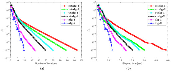
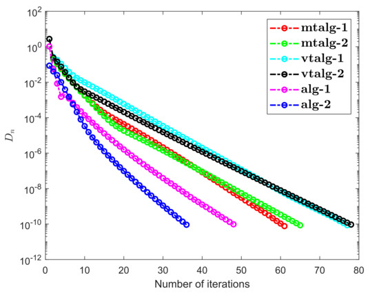
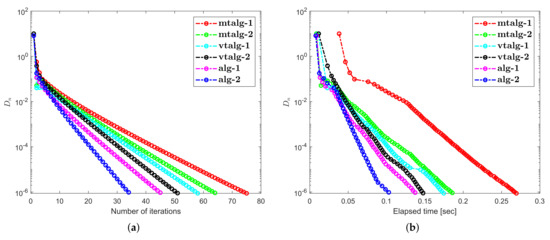
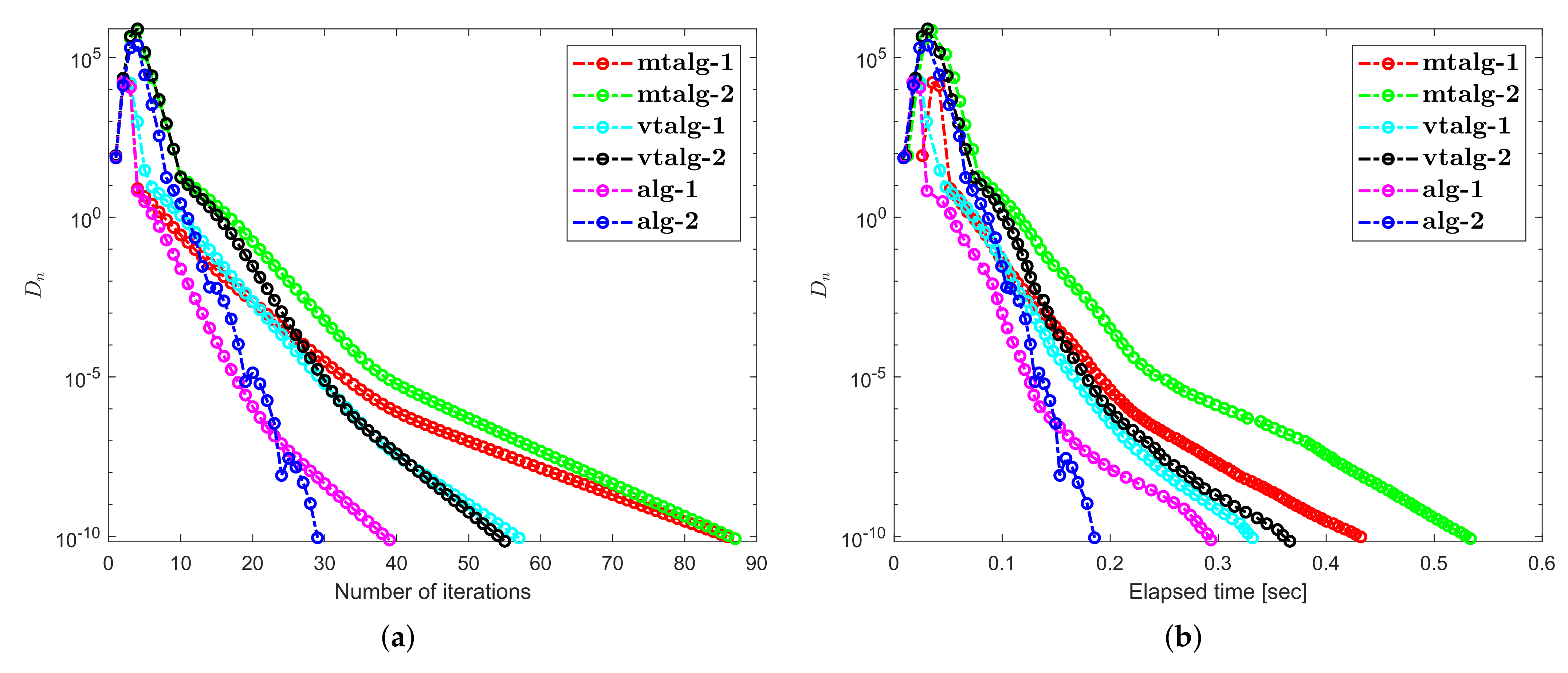
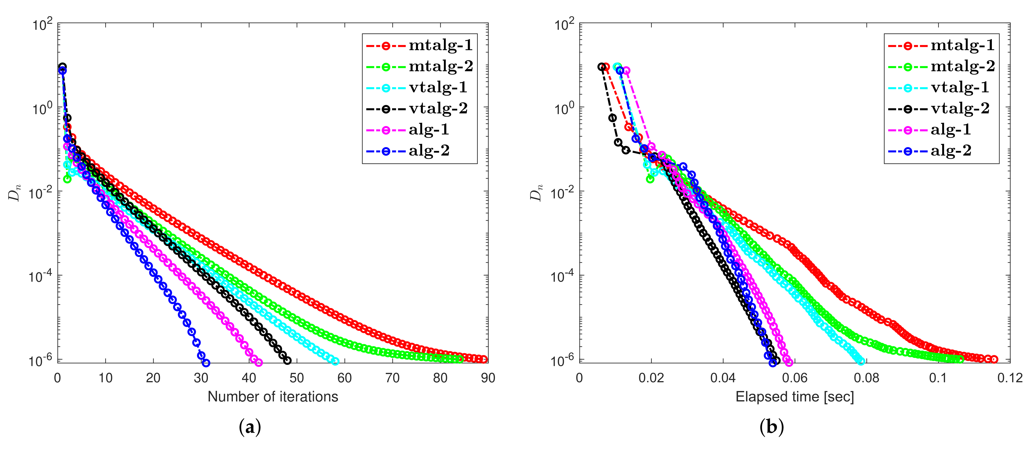
It is obvious that ℑ is monotone and that Lipschitz is continuous by $L=\parallel M\parallel .$ Let $\mathcal{T}:\mathcal{X}\to \mathcal{X}$ be provided by $\mathcal{T}u=\frac{1}{2}u.$ The starting point for this experiment are $u_0=u_1=(2,2,\cdots ,2)$ and dimension of the space is taken differently with stopping criterion $D_k=\parallel t_k-y_k\parallel \le {10}^{-10}.$ Numerical observations for Example 1 are shown in Figure 1, Figure 2, Figure 3 and Figure 4 and Table 1 and Table 2. Control criteria applied are as follows: (1) Algorithm 1 (shortly, alg-1): ${\gimel }_1=0.55,\theta =0.45,\mu =0.44,{ϵ}_k=\frac{100}{{(1+k)}^2},{\beta }_k=\frac{1}{(2k+4)},{\alpha }_k=\frac{k}{(2k+1)}.$ (2) Algorithm 2 (shortly, alg-2): ${\gimel }_1=0.55,\theta =0.45,\mu =0.44,{ϵ}_k=\frac{100}{{(1+k)}^2},{\beta }_k=\frac{1}{(2k+4)},{\alpha }_k=\frac{k}{(2k+1)}.$ (3) Algorithm 1 in [36] (shortly, mtalg-1): ${\gamma }_1=0.55,\delta =0.45,\varphi =0.44,{\theta }_k=\frac{1}{(2k+4)},{\gimel }_k=\frac{1}{2}(1-{\theta }_k),{ϵ}_k=\frac{100}{{(1+k)}^2}.$ (4) Algorithm 2 in [36] (shortly, mtalg-2): ${\gamma }_1=0.55,\delta =0.45,\varphi =0.44,{\theta }_k=\frac{1}{(2k+4)},{\gimel }_k=\frac{1}{2}(1-{\theta }_k),{ϵ}_k=\frac{100}{{(1+k)}^2}.$ (5) Algorithm 1 in [35] (shortly, vtalg-1): ${\tau }_1=0.55,\theta =0.45,\mu =0.44,{ϵ}_k=\frac{100}{{(1+k)}^2},{\beta }_k=\frac{1}{(2k+4)},{\alpha }_k=\frac{k}{(2k+1)},f\left(u\right)=\frac{u}{2}.$ (6) Algorithm 2 in [35] (shortly, vtalg-2): ${\tau }_1=0.55,\theta =0.45,\mu =0.44,{ϵ}_k=\frac{100}{{(1+k)}^2},{\beta }_k=\frac{1}{(2k+4)},{\alpha }_k=\frac{k}{(2k+1)},f\left(u\right)=\frac{u}{2}.$

Figure 1. Computational illustration of Algorithms 1 and 2 with Algorithm 1 in [36], Algorithm 2 in [36] and Algorithm 1 in [35], Algorithm 2 in [35] when $m=5$.

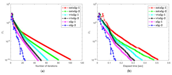
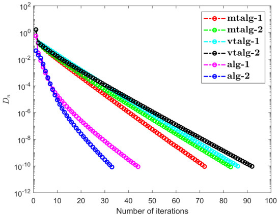
Figure 2. Computational illustration of Algorithms 1 and 2 with Algorithm 1 in [36], Algorithm 2 in [36] and Algorithm 1 in [35], Algorithm 2 in [35] when $m=10$.

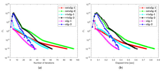
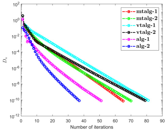
Figure 3. Computational illustration of Algorithms 1 and 2 with Algorithm 1 in [36], Algorithm 2 in [36] and Algorithm 1 in [35], Algorithm 2 in [35] when $m=50$.

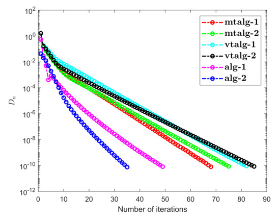
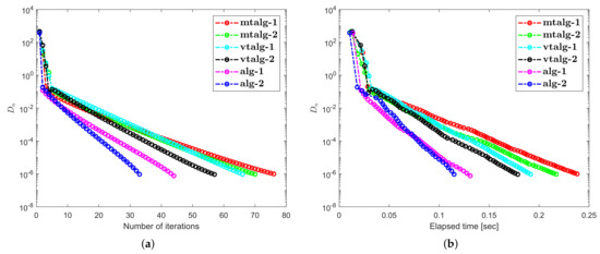
Figure 4. Computational illustration of Algorithms 1 and 2 with Algorithm 1 in [36], Algorithm 2 in [36] and Algorithm 1 in [35], Algorithm 2 in [35] when $m=200$.

Table 1. Example 1 obtained numerical values.

		Total Number of Iterations
$\mathit{m}$	alg-1	alg-2	mtalg-1	mtalg-2	vtalg-1	vtalg-2
5	36	19	94	78	60	49
10	46	24	102	80	62	51
20	42	25	93	85	59	53
50	38	25	86	87	57	55
100	37	32	84	88	56	56
200	38	36	84	94	56	62

Table 2. Example 1 obtained numerical values.

		Required CPU Time
$\mathit{m}$	alg-1	alg-2	mtalg-1	mtalg-2	vtalg-1	vtalg-2
5	0.246841	0.1317703	0.5865135	0.4009539	0.360533465	0.3001653
10	0.284076	0.1523123	0.5159276	0.4722816	0.375091336	0.3097725
20	0.2602246	0.1633652	0.4246998	0.4630932	0.393142367	0.3358743
50	0.293302	0.1854808	0.4320612	0.5335381	0.331728156	0.3663686
100	0.2566573	0.2301228	0.4752024	0.5067862	0.358997537	0.3936471
200	0.3544296	0.3695034	0.7371152	0.8441844	0.516623963	0.6142675

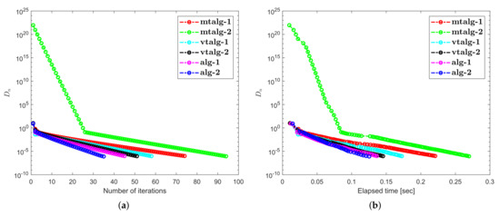
Example  2.

Consider a nonlinear operator $\Im :{\mathcal{R}}^2\to {\mathcal{R}}^2$ is defined by

$$\Im (u,y)=(u+y+sinu;-u+y+siny)$$

and the feasible set $\mathcal{Y}$ is a set expressed by $\mathcal{Y}=[-1,1]\times [-1,1]$. It is easy to check that ℑ is monotone and Lipschitz continuous with the constant $L=3$. Let E be a $2\times 2$ matrix defined by

$$E=\left(\begin{array}{cc}1& 0\\ 0& 2\end{array}\right)$$

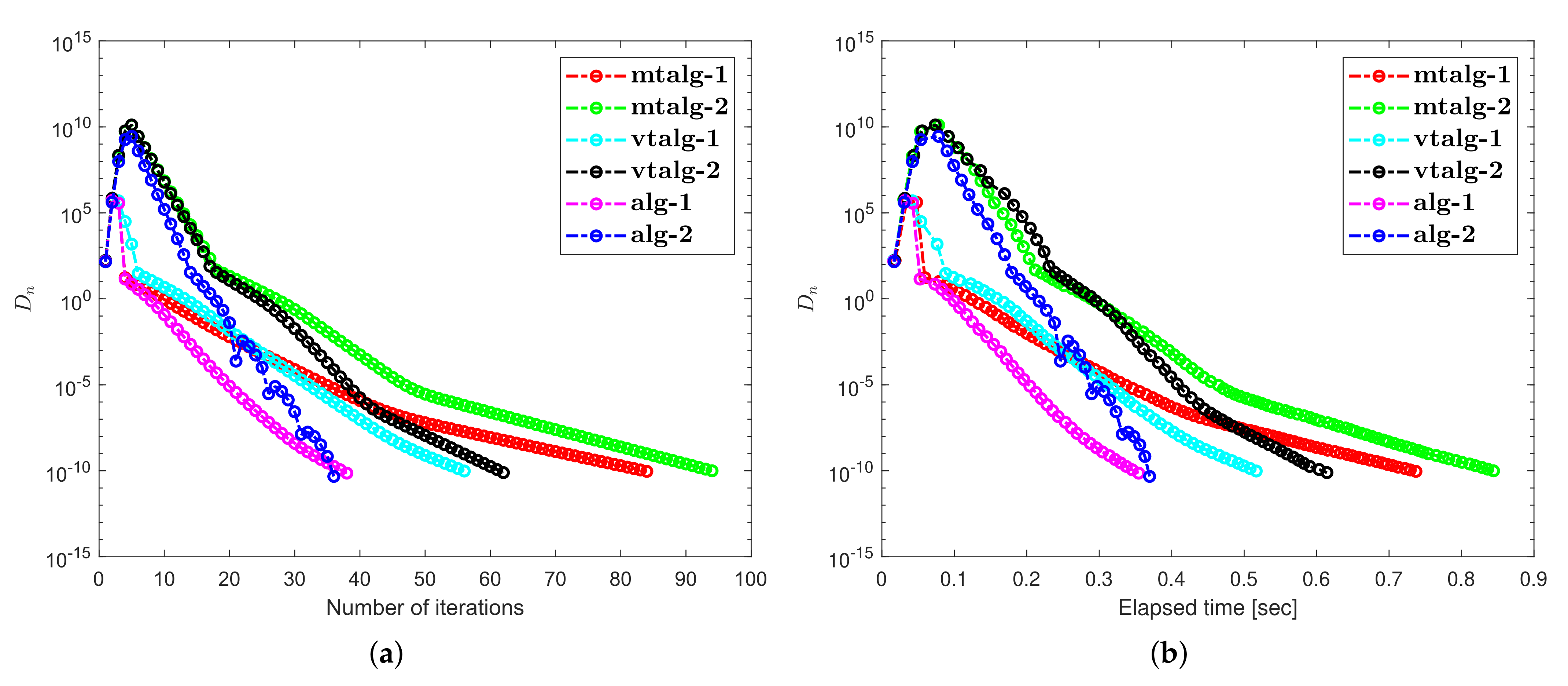
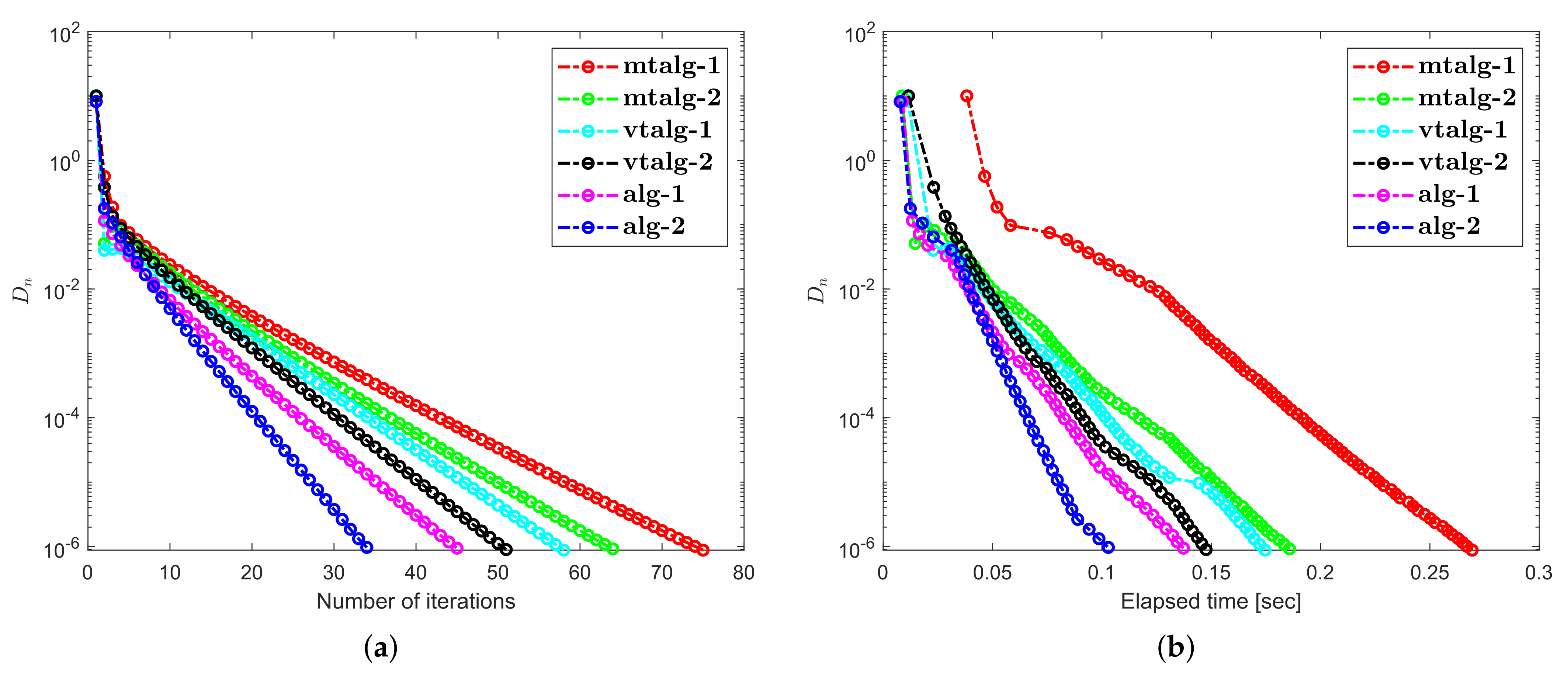
We consider the mapping $\mathcal{T}:{\mathcal{R}}^2\to {\mathcal{R}}^2$ by $\mathcal{T}z={\parallel E\parallel }^{-1}Ez,$ where $z={(u,y)}^T.$ It is obvious to see that $\mathcal{T}$ is 0-demicontractive and thus $\rho =0.$ The solution of the problem is $r^{*}={(0,0)}^T.$ The starting points for this experiment are used differently with stopping criterion $D_k=\parallel t_k-y_k\parallel \le {10}^{-10}.$ Numerical observations for Example 2 are shown in Figure 5, Figure 6, Figure 7 and Figure 8 and Table 3 and Table 4. Control criteria applied are as follows: (1) Algorithm 1 (shortly, alg-1): ${\gimel }_1=0.45,\theta =0.35,\mu =0.33,{ϵ}_k=\frac{10}{{(1+k)}^2},{\beta }_k=\frac{1}{(3k+6)},{\alpha }_k=\frac{k}{(3k+1)}.$ (2) Algorithm 2 (shortly, alg-2): ${\gimel }_1=0.45,\theta =0.35,\mu =0.33,{ϵ}_k=\frac{10}{{(1+k)}^2},{\beta }_k=\frac{1}{(3k+4)},{\alpha }_k=\frac{k}{(3k+1)}.$ (3) Algorithm 1 in [36] (shortly, mtalg-1): ${\gamma }_1=0.45,\delta =0.35,\varphi =0.33,{\theta }_k=\frac{1}{(3k+6)},{\gimel }_k=\frac{1}{2.5}(1-{\theta }_k),{ϵ}_k=\frac{10}{{(1+k)}^2}.$ (4) Algorithm 2 in [36] (shortly, mtalg-2): ${\gamma }_1=0.45,\delta =0.35,\varphi =0.33,{\theta }_k=\frac{1}{(3k+6)},{\gimel }_k=\frac{1}{2.5}(1-{\theta }_k),{ϵ}_k=\frac{10}{{(1+k)}^2}.$ (5) Algorithm 1 in [35] (shortly, vtalg-1): ${\tau }_1=0.45,\theta =0.35,\mu =0.33,{ϵ}_k=\frac{10}{{(1+k)}^2},{\beta }_k=\frac{1}{(3k+6)},{\alpha }_k=\frac{k}{(3k+1)},f\left(u\right)=\frac{u}{2}.$ (6) Algorithm 2 in [35] (shortly, vtalg-2): ${\tau }_1=0.45,\theta =0.35,\mu =0.33,{ϵ}_k=\frac{10}{{(1+k)}^2},{\beta }_k=\frac{1}{(3k+6)},{\alpha }_k=\frac{k}{(3k+1)},f\left(u\right)=\frac{u}{2}.$

Figure 5. Computational illustration of Algorithms 1 and 2 with Algorithm 1 in [36], Algorithm 2 in [36] and Algorithm 1 in [35], Algorithm 2 in [35] when $u_0=u_1={(1,1)}^T$.

Figure 6. Computational illustration of Algorithms 1 and 2 with Algorithm 1 in [36], Algorithm 2 in [36] and Algorithm 1 in [35], Algorithm 2 in [35] when $u_0=u_1={(2,2)}^T$.

Figure 7. Computational illustration of Algorithms 1 and 2 with Algorithm 1 in [36], Algorithm 2 in [36] and Algorithm 1 in [35], Algorithm 2 in [35] when $u_0=u_1={(1,-1)}^T$.

Figure 8. Computational illustration of Algorithms 1 and 2 with Algorithm 1 in [36], Algorithm 2 in [36] and Algorithm 1 in [35], Algorithm 2 in [35] when $u_0=u_1={(-2,-3)}^T$.

Table 3. Example 2 obtained numerical values.

		Total Number of Iterations
${\mathit{u}}_0={\mathit{u}}_1$	alg-1	alg-2	mtalg-1	mtalg-2	vtalg-1	vtalg-2
${(1,1)}^T$	49	35	68	75	82	85
${(2,2)}^T$	48	36	61	65	77	78
${(1,-1)}^T$	44	33	72	83	86	92
${(-2,3)}^T$	51	37	65	70	81	79

Table 4. Example 2 obtained numerical values.

		Required CPU Time
${\mathit{u}}_0={\mathit{u}}_1$	alg-1	alg-2	mtalg-1	mtalg-2	vtalg-1	vtalg-2
${(1,1)}^T$	0.2284193	0.1631707	0.2969821	0.3224385	0.3469049	0.3625844
${(2,2)}^T$	0.2297859	0.1757931	0.3720656	0.3078242	0.3847476	0.4105755
${(1,-1)}^T$	0.1986126	0.1512495	0.3220028	0.3729462	0.3787876	0.4068135
${(-2,3)}^T$	0.2380988	0.1703252	0.2690971	0.3069672	0.3448697	0.3428332

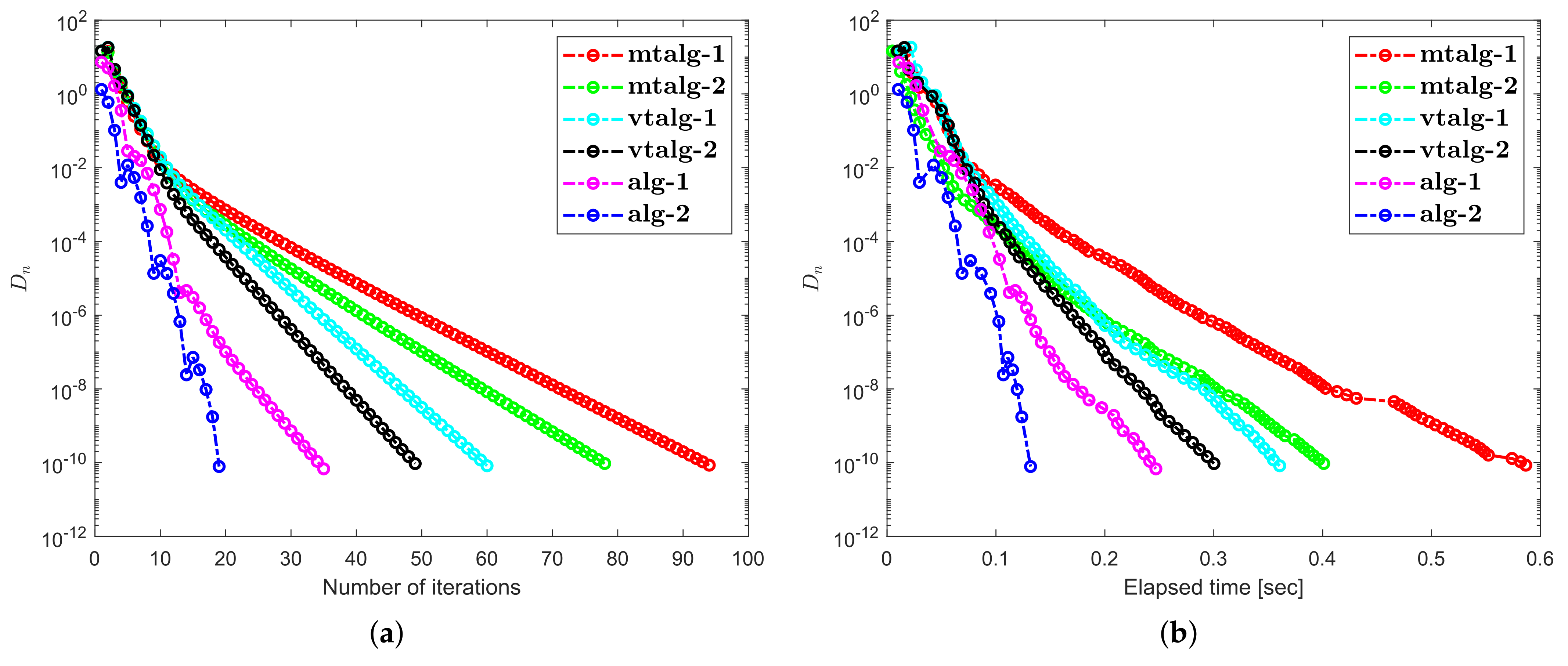
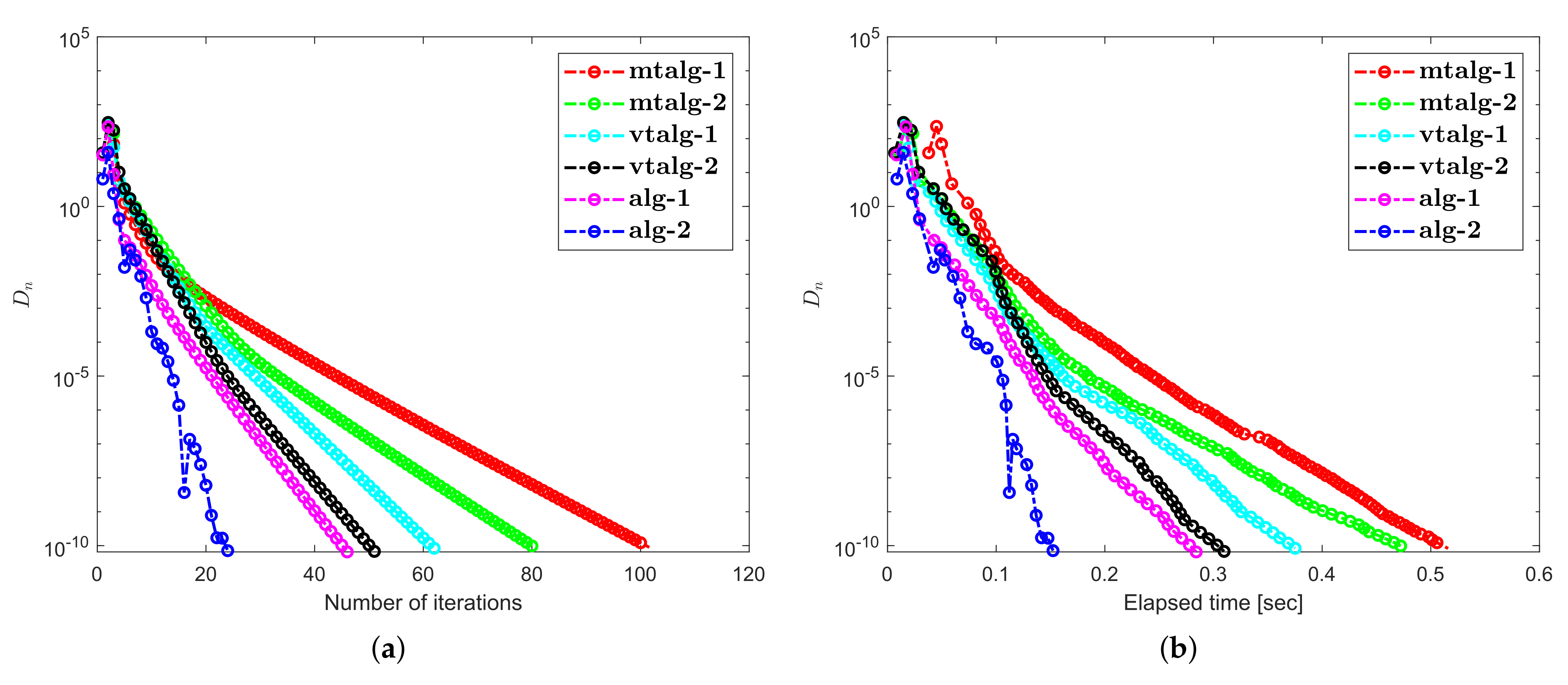
Example  3.

Suppose that $\mathcal{X}=L^2\left([0,1]\right)$ be a Hilbert space through an inner product

$$⟨u,y⟩={\int }_0^{1}u\left(t\right)y\left(t\right)dt,\forall u,y\in \mathcal{X},$$

where the induced norm

$$\parallel u\parallel =\sqrt{{\int }_0^1{\left|u\left(t\right)\right|}^{2}dt}.$$

Let $\mathcal{Y}:=\{u\in L^2\left([0,1]\right):\parallel u\parallel \le 1\}$ be the unit ball and $\Im :\mathcal{Y}\to \mathcal{X}$ is defined by

$$\Im \left(u\right)\left(t\right)={\int }_0^1\left(u\left(t\right)-H(t,s)f\left(u\right(s\left)\right)\right)ds+g\left(t\right),$$

where

$$H(t,s)=\frac{2ts{e}^{(t+s)}}{e\sqrt{e^2-1}},f\left(u\right)=cosu,g\left(t\right)=\frac{2t{e}^t}{e\sqrt{e^2-1}}.$$

It is evident that ℑ is Lipschitz-continuous with Lipschitz constant $L=2$ and monotone [44]. The projection on $\mathcal{Y}$ is inherently explicit, that is,

$$P_C\left(u\right)=\left\{\begin{array}{c}\frac{u}{\parallel u\parallel }\mathrm{if}\parallel u\parallel >1,\hfill \\ \\ u,\parallel u\parallel \le 1.\hfill \end{array}\right.$$

An operator $\mathcal{T}:L^2\left([0,1]\right)\to L^2\left([0,1]\right)$ is of form

$$\mathcal{T}\left(u\right)\left(t\right)={\int }_0^{1}tu\left(s\right)ds,t\in [0,1].$$

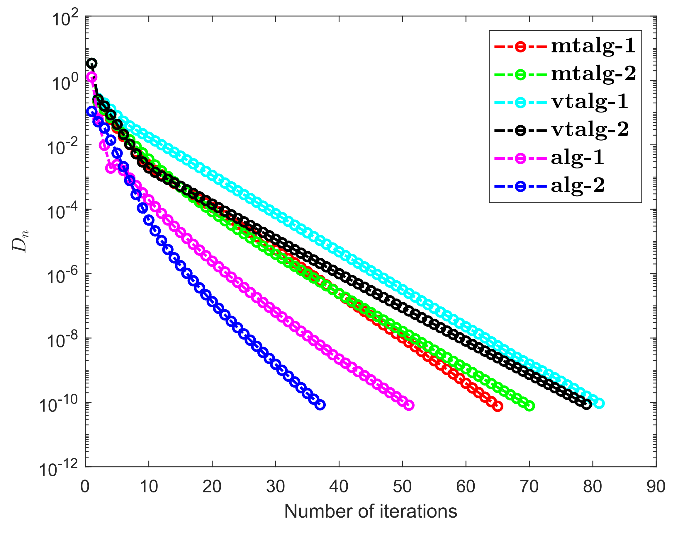
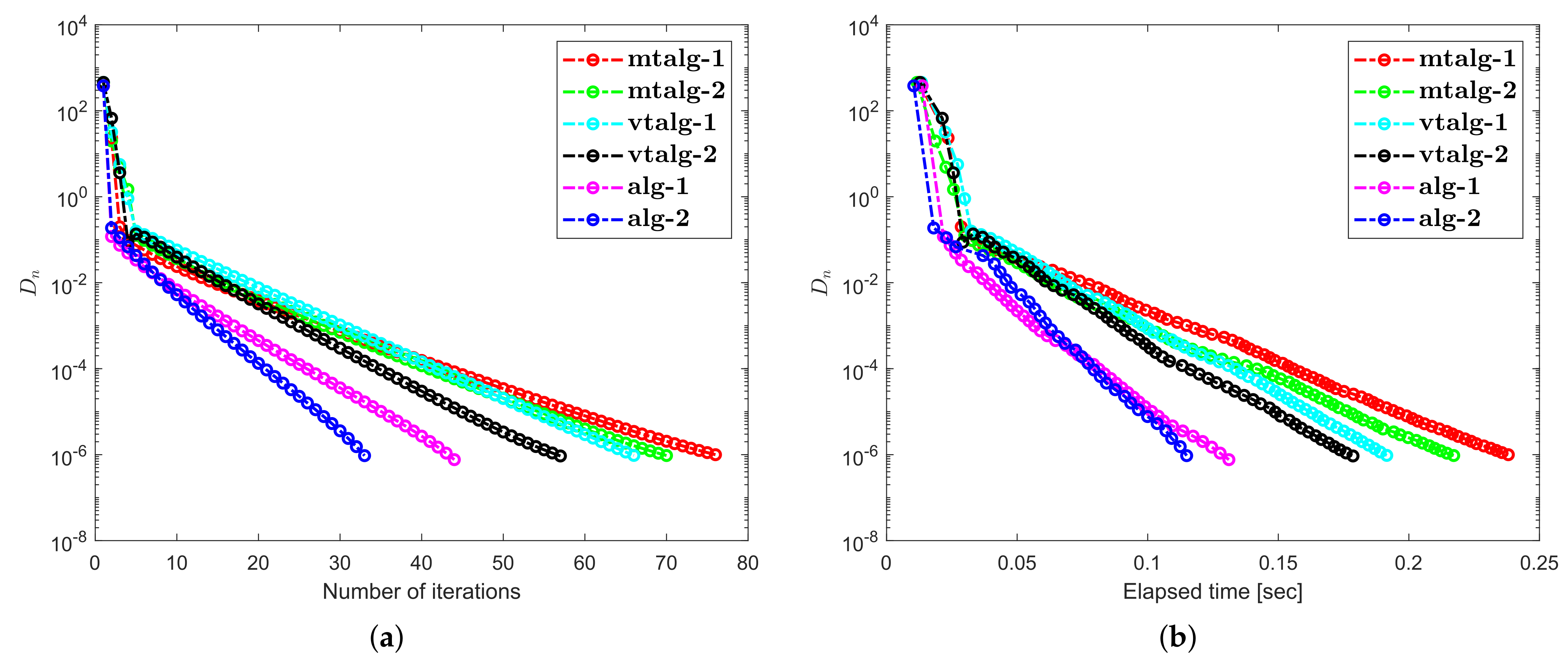
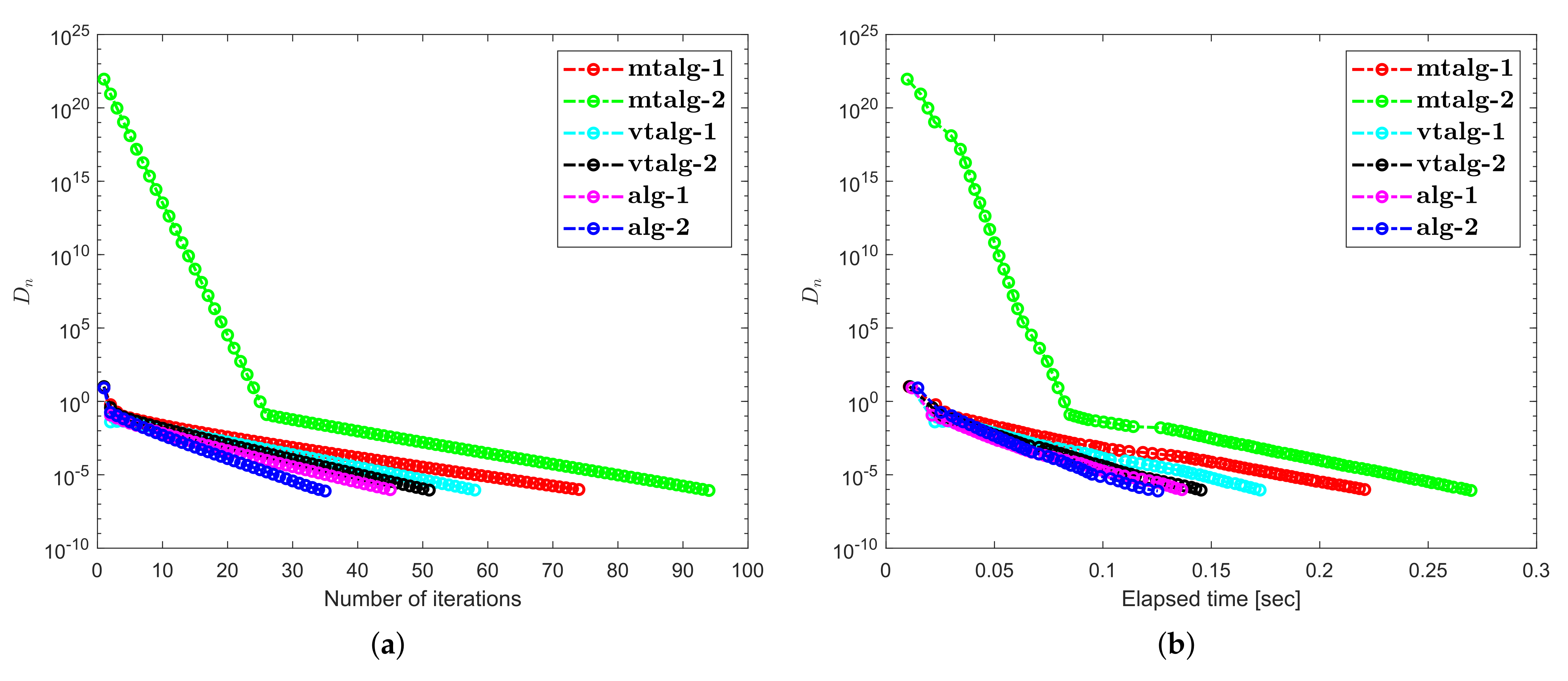
A straightforward computation implies that $\mathcal{T}$ is 0-demicontractive. The solution of the problem is $r^{*}\left(t\right)=0.$ The starting point for this experiment are taken differently with stopping criterion $D_k=\parallel t_k-y_k\parallel \le {10}^{-6}.$ Numerical observations for Example 3 are shown in Figure 9, Figure 10, Figure 11 and Figure 12 and Table 5 and Table 6. Control criteria applied are as follows: (1) Algorithm 1 (shortly, alg-1): ${\gimel }_1=0.33,\theta =0.66,\mu =0.55,{ϵ}_k=\frac{1}{{(1+k)}^2},{\beta }_k=\frac{1}{(4k+8)},{\alpha }_k=\frac{k}{(5k+1)}.$ (2) Algorithm 2 (shortly, alg-2): ${\gimel }_1=0.33,\theta =0.66,\mu =0.55,{ϵ}_k=\frac{1}{{(1+k)}^2},{\beta }_k=\frac{1}{(4k+8)},{\alpha }_k=\frac{k}{(5k+1)}.$ (3) Algorithm 1 in [36] (shortly, mtalg-1): ${\gamma }_1=0.33,\delta =0.66,\varphi =0.55,{\theta }_k=\frac{1}{(4k+8)},{\gimel }_k=\frac{1}{2}(1-{\theta }_k),{ϵ}_k=\frac{1}{{(1+k)}^2}.$ (4) Algorithm 2 in [36] (shortly, mtalg-2): ${\gamma }_1=0.33,\delta =0.66,\varphi =0.55,{\theta }_k=\frac{1}{(4k+8)},{\gimel }_k=\frac{1}{2}(1-{\theta }_k),{ϵ}_k=\frac{1}{{(1+k)}^2}.$ (5) Algorithm 1 in [35] (shortly, vtalg-1): ${\tau }_1=0.33,\theta =0.66,\mu =0.55,{ϵ}_k=\frac{1}{{(1+k)}^2},{\beta }_k=\frac{1}{(4k+8)},{\alpha }_k=\frac{k}{(4k+1)},f\left(u\right)=\frac{u}{3}.$ (6) Algorithm 2 in [35] (shortly, vtalg-2): ${\tau }_1=0.33,\theta =0.66,\mu =0.55,{ϵ}_k=\frac{1}{{(1+k)}^2},{\beta }_k=\frac{1}{(4k+8)},{\alpha }_k=\frac{k}{(4k+1)},f\left(u\right)=\frac{u}{3}.$

Figure 9. Computational illustration of Algorithms 1 and 2 with Algorithm 1 in [36], Algorithm 2 in [36] and Algorithm 1 in [35], Algorithm 2 in [35] when $u_0=1$.

Figure 10. Computational illustration of Algorithms 1 and 2 with Algorithm 1 in [36], Algorithm 2 in [36] and Algorithm 1 in [35], Algorithm 2 in [35] when $u_0=u_1=t$.

Figure 11. Computational illustration of Algorithms 1 and 2 with Algorithm 1 in [36], Algorithm 2 in [36] and Algorithm 1 in [35], Algorithm 2 in [35] when $u_0=u_1=sin\left(t\right)$.

Figure 12. Computational illustration of Algorithms 1 and 2 with Algorithm 1 in [36], Algorithm 2 in [36] and Algorithm 1 in [35], Algorithm 2 in [35] when $u_0=u_1=cos\left(t\right)$.

Table 5. Example 3 obtained numerical values.

		Total Number of Iterations
${\mathit{u}}_0={\mathit{u}}_1$	alg-1	alg-2	mtalg-1	mtalg-2	vtalg-1	vtalg-2
1	44	33	76	70	66	57
t	42	31	89	84	58	48
$sin\left(t\right)$	45	34	75	64	58	51
$cos\left(t\right)$	47	35	74	94	58	51

Table 6. Example 3 obtained numerical values.

		Required CPU Time
${\mathit{u}}_0={\mathit{u}}_1$	alg-1	alg-2	mtalg-1	mtalg-2	vtalg-1	vtalg-2
1	0.1310831	0.1149104	0.2380825	0.2171721	0.1915358	0.178602
t	0.0583617	0.0538350	0.1154974	0.1059993	0.0784157	0.0548289
$sin\left(t\right)$	0.1372786	0.1029274	0.2692971	0.185825	0.1745996	0.1476468
$cos\left(t\right)$	0.1364229	0.1253482	0.2207376	0.2697567	0.172504	0.1452834

5. Discussion about Numerical Illustrations

Regarding the above-mentioned numerical experiments, we have the following findings:

(1)

Examples 1–3 reported results for several algorithms in both finite and infinite-dimensional spaces. It is clear to see that the provided algorithms outperformed in terms of number of iterations and elapsed time in almost all situations. All experiments show that the proposed algorithms perform better the previously existing algorithms.

(2)

The appearance of unsuitable variable step size causes a hump in the graph of algorithms in Example 2. It does not really effect the overall performance of the algorithms.

(3)

Examples 1–3 reported results for different algorithms for both finite and infinite-dimensional spaces. In most cases, we can see that the algorithm’s performance is determined by the nature of the problem and the tolerance value employed.

(4)

For large-dimensional problems, all approaches typically took longer and showed significant variation in execution time. The number of iterations, on the other hand, changes slightly less.

(5)

It is also observed that a specific formula for stepsize evaluation enhances the algorithm’s efficiency and the pace of convergence. In other words, rather than the fixed stepsize, the appropriate variable stepsize improves the performance of algorithms.

(6)

In Examples 2 and 3, it can also be shown that the initial point choice and the complexity of the operators have an influence on the performance of algorithms in terms of the number of iterations and time of execution in seconds.

References

- Maingé, P.E. A Hybrid Extragradient-Viscosity Method for Monotone Operators and Fixed Point Problems. SIAM J. Control. Optim. 2008, 47, 1499–1515. [Google Scholar] [CrossRef]
- Maingé, P.E.; Moudafi, A. Coupling viscosity methods with the extragradient algorithm for solving equilibrium problems. J. Nonlinear Convex Anal. 2008, 9, 283–294. [Google Scholar]
- Iiduka, H.; Yamada, I. A subgradient-type method for the equilibrium problem over the fixed point set and its applications. Optimization 2009, 58, 251–261. [Google Scholar] [CrossRef]
- Qin, X.; An, N.T. Smoothing algorithms for computing the projection onto a Minkowski sum of convex sets. Comput. Optim. Appl. 2019, 74, 821–850. [Google Scholar] [CrossRef] [Green Version]
- An, N.T.; Nam, N.M.; Qin, X. Solving k-center problems involving sets based on optimization techniques. J. Glob. Optim. 2019, 76, 189–209. [Google Scholar] [CrossRef]
- Stampacchia, G. Formes bilinéaires coercitives sur les ensembles convexes. Comptes Rendus Hebd. Des Seances Acad. Des Sci. 1964, 258, 4413. [Google Scholar]
- Konnov, I.V. On systems of variational inequalities. Russ. Math. C/C -Izv.-Vyss. Uchebnye Zaved. Mat. 1997, 41, 77–86. [Google Scholar]
- Kassay, G.; Kolumbán, J.; Páles, Z. On Nash stationary points. Publ. Math. 1999, 54, 267–279. [Google Scholar]
- Kassay, G.; Kolumbán, J.; Páles, Z. Factorization of Minty and Stampacchia variational inequality systems. Eur. J. Oper. Res. 2002, 143, 377–389. [Google Scholar] [CrossRef]
- Kinderlehrer, D.; Stampacchia, G. An Introduction to Variational Inequalities and Their Applications; Society for Industrial and Applied Mathematics: Philadelphia, PA, USA, 2000. [Google Scholar] [CrossRef]
- Konnov, I. Equilibrium Models and Variational Inequalities; Elsevier: Amsterdam, The Netherlands, 2007; Volume 210. [Google Scholar]
- Elliott, C.M. Variational and Quasivariational Inequalities Applications to Free—Boundary ProbLems. (Claudio Baiocchi Furthermore, António Capelo). SIAM Rev. 1987, 29, 314–315. [Google Scholar] [CrossRef]
- Nagurney, A. Network Economics: A Variational Inequality Approach; Kluwer Academic Publishers Group: Dordrecht, The Netherlands, 1999. [Google Scholar] [CrossRef]
- Takahashi, W. Introduction to Nonlinear and Convex Analysis; Yokohama Publishers: Yokohama, Japan, 2009. [Google Scholar]
- Korpelevich, G. The extragradient method for finding saddle points and other problems. Matecon 1976, 12, 747–756. [Google Scholar]
- Noor, M.A. Some iterative methods for nonconvex variational inequalities. Comput. Math. Model. 2010, 21, 97–108. [Google Scholar] [CrossRef]
- Censor, Y.; Gibali, A.; Reich, S. The subgradient extragradient method for solving variational inequalities in Hilbert space. J. Optim. Theory Appl. 2010, 148, 318–335. [Google Scholar] [CrossRef] [PubMed] [Green Version]
- Censor, Y.; Gibali, A.; Reich, S. Extensions of Korpelevich extragradient method for the variational inequality problem in Euclidean space. Optimization 2012, 61, 1119–1132. [Google Scholar] [CrossRef]
- Tseng, P. A Modified Forward-Backward Splitting Method for Maximal Monotone Mappings. SIAM J. Control. Optim. 2000, 38, 431–446. [Google Scholar] [CrossRef]
- Moudafi, A. Viscosity Approximation Methods for Fixed-Points Problems. J. Math. Anal. Appl. 2000, 241, 46–55. [Google Scholar] [CrossRef] [Green Version]
- Zhang, L.; Fang, C.; Chen, S. An inertial subgradient-type method for solving single-valued variational inequalities and fixed point problems. Numer. Algorithms 2018, 79, 941–956. [Google Scholar] [CrossRef]
- Iusem, A.N.; Svaiter, B.F. A variant of korpelevich’s method for variational inequalities with a new search strategy. Optimization 1997, 42, 309–321. [Google Scholar] [CrossRef]
- Thong, D.V.; Hieu, D.V. Modified subgradient extragradient method for variational inequality problems. Numer. Algorithms 2017, 79, 597–610. [Google Scholar] [CrossRef]
- Thong, D.V.; Hieu, D.V. Weak and strong convergence theorems for variational inequality problems. Numer. Algorithms 2017, 78, 1045–1060. [Google Scholar] [CrossRef]
- Rehman, H.; Kumam, P.; Shutaywi, M.; Alreshidi, N.A.; Kumam, W. Inertial optimization based two-step methods for solving equilibrium problems with applications in variational inequality problems and growth control equilibrium models. Energies 2020, 13, 3292. [Google Scholar] [CrossRef]
- Hammad, H.A.; Rehman, H.; la Sen, M.D. Advanced algorithms and common solutions to variational inequalities. Symmetry 2020, 12, 1198. [Google Scholar] [CrossRef]
- Yordsorn, P.; Kumam, P.; Rehman, H.; Ibrahim, A.H. A weak convergence self-adaptive method for solving pseudomonotone equilibrium problems in a real Hilbert space. Mathematics 2020, 8, 1165. [Google Scholar] [CrossRef]
- Rehman, H.; Gibali, A.; Kumam, P.; Sitthithakerngkiet, K. Two new extragradient methods for solving equilibrium problems. Rev. Real Acad. Cienc. Exactas Fis. Nat. Ser. Mat. 2021, 115. [Google Scholar] [CrossRef]
- Rehman, H.; Kumam, P.; Gibali, A.; Kumam, W. Convergence analysis of a general inertial projection-type method for solving pseudomonotone equilibrium problems with applications. J. Inequalities Appl. 2021, 2021. [Google Scholar] [CrossRef]
- Rehman, H.; Alreshidi, N.A.; Muangchoo, K. A New Modified Subgradient Extragradient Algorithm Extended for Equilibrium Problems with Application in Fixed Point Problems. J. Nonlinear Convex Anal. 2021, 22, 421–439. [Google Scholar]
- Muangchoo, K.; Rehman, H.; Kumam, P. Weak convergence and strong convergence of nonmonotonic explicit iterative methods for solving equilibrium problems. J. Nonlinear Convex Anal. 2021, 22, 663–681. [Google Scholar]
- Rehman, H.; Kumam, P.; Özdemir, M.; Karahan, I. Two generalized non-monotone explicit strongly convergent extragradient methods for solving pseudomonotone equilibrium problems and applications. Math. Comput. Simul. 2021. [Google Scholar] [CrossRef]
- Antipin, A.S. On a method for convex programs using a symmetrical modification of the Lagrange function. Ekon. Mat. Metod. 1976, 12, 1164–1173. [Google Scholar]
- Yamada, I.; Ogura, N. Hybrid Steepest Descent Method for Variational Inequality Problem over the Fixed Point Set of Certain Quasi-nonexpansive Mappings. Numer. Funct. Anal. Optim. 2005, 25, 619–655. [Google Scholar] [CrossRef]
- Tan, B.; Zhou, Z.; Li, S. Viscosity-type inertial extragradient algorithms for solving variational inequality problems and fixed point problems. J. Appl. Math. Comput. 2021. [Google Scholar] [CrossRef]
- Tan, B.; Fan, J.; Qin, X. Inertial extragradient algorithms with non-monotonic step sizes for solving variational inequalities and fixed point problems. Adv. Oper. Theory 2021, 6. [Google Scholar] [CrossRef]
- Mann, W.R. Mean value methods in iteration. Proc. Am. Math. Soc. 1953, 4, 506. [Google Scholar] [CrossRef]
- Zhou, H.; Qin, X. Fixed Points of Nonlinear Operators; De Gruyter: Berlin, Germany, 2020. [Google Scholar]
- Saejung, S.; Yotkaew, P. Approximation of zeros of inverse strongly monotone operators in Banach spaces. Nonlinear Anal. Theory Methods Appl. 2012, 75, 742–750. [Google Scholar] [CrossRef]
- Hicks, T.L.; Kubicek, J.D. On the Mann iteration process in a Hilbert space. J. Math. Anal. Appl. 1977, 59, 498–504. [Google Scholar] [CrossRef] [Green Version]
- Karamardian, S. Complementarity problems over cones with monotone and pseudomonotone maps. J. Optim. Theory Appl. 1976, 18, 445–454. [Google Scholar] [CrossRef]
- Harker, P.T.; Pang, J.S. A damped-Newton method for the linear complementarity problem. Comput. Solut. Nonlinear Syst. Equ. 1990, 26, 265. [Google Scholar]
- Solodov, M.V.; Svaiter, B.F. A New Projection Method for Variational Inequality Problems. SIAM J. Control. Optim. 1999, 37, 765–776. [Google Scholar] [CrossRef]
- Van Hieu, D.; Anh, P.K.; Muu, L.D. Modified hybrid projection methods for finding common solutions to variational inequality problems. Comput. Optim. Appl. 2016, 66, 75–96. [Google Scholar] [CrossRef]
- Dong, Q.L.; Cho, Y.J.; Zhong, L.L.; Rassias, T.M. Inertial projection and contraction algorithms for variational inequalities. J. Glob. Optim. 2017, 70, 687–704. [Google Scholar] [CrossRef]
Publisher’s Note: MDPI stays neutral with regard to jurisdictional claims in published maps and institutional affiliations. |
© 2022 by the authors. Licensee MDPI, Basel, Switzerland. This article is an open access article distributed under the terms and conditions of the Creative Commons Attribution (CC BY) license (https://creativecommons.org/licenses/by/4.0/).