A Hybrid Localized Meshless Method for the Solution of Transient Groundwater Flow in Two Dimensions

Abstract

In this work, a hybrid localized meshless method is developed for solving transient groundwater flow in two dimensions by combining the Crank–Nicolson scheme and the generalized finite difference method (GFDM). As the first step, the temporal discretization of the transient groundwater flow equation is based on the Crank–Nicolson scheme. A boundary value problem in space with the Dirichlet or mixed boundary condition is then formed at each time node, which is simulated by introducing the GFDM. The proposed algorithm is truly meshless and easy to program. Four linear or nonlinear numerical examples, including ones with complicated geometry domains, are provided to verify the performance of the developed approach, and the results illustrate the good accuracy and convergency of the method.

1. Introduction

As an important component of the hydrological cycle system, groundwater is a key source of domestic and industrial water supply. Therefore, the analysis of the groundwater flow has great significance for water supply security. Due to the complexity of the problem, an analytical solution is rarely available for most models of groundwater flow. With the development of computing techniques, more and more numerical approaches have been developed and applied to numerical simulations of science and engineering problems, such as the finite element method (FEM) [1,2,3], the boundary element method (BEM) [4,5], and the meshless method [6,7,8,9,10].

As a new approach in recent years, the meshless method is now widely applied in various fields [11,12,13,14,15,16,17,18,19], particularly in computational fluid dynamics (CFD). The developed meshless approaches can be classified into collocation-based and Galerkin-based methods. Compared with the latter, the meshless collocation methods have the advantages of no numerical quadrature and mesh generation, and some of these are the localized method of fundamental solutions (LMFS) [20,21,22], the generalized finite difference method (GFDM) [23,24,25,26,27,28,29,30,31,32,33], the localized Chebyshev collocation method [34], the singular boundary method (SBM) [35,36,37,38,39,40,41,42,43], and the localized knot method (LKM) [44].

The GFDM, as a popular localized meshless collocation method, employs the Taylor series expansions and moving least squares (MLS) approximations [45,46] to form the system of algebraic equations with a spare matrix [47,48]. Thanks to this spare system, this method is highly efficient and suitable for the numerical simulations of large-scale problems. Many physical applications have been addressed by the GFDM, such as the thin elastic plate bending analysis [49], the electroelastic analysis of 3D piezoelectric structures [50], the acoustic wave propagation [51], the inverse Cauchy problem in 2D elasticity [52], the heat conduction problems [53], and the stationary flow in a dam [54].

A hybrid localized meshless method is proposed in this paper for the solution of transient groundwater flow in a two-dimensional space by combining the Crank–Nicolson scheme and the GFDM. As the first step, the Crank–Nicolson scheme is applied to the temporal discretization of the transient groundwater flow equation. At each time node, a boundary value problem in space is then formed and subsequently solved with the GFDM. Through the above process, a hybrid localized meshless approach is finally established, which is truly meshless and easy to program. The rest of the work is organized as follows. The governing equation of transient groundwater flow with boundary and initial conditions is described in Section 2. The formulations of the hybrid localized meshless method are derived in Section 3. Several linear and nonlinear numerical examples are provided in Section 4 to verify the performance of the developed method. Some conclusions are presented in Section 5.

2. Problem Definition

The movement of transient groundwater flow of a constant density in a homogeneous and anisotropic two-dimensional (2D) medium with the domain $\mathsf{\Omega }$ can be described by using the following equation:

$$T_x\frac{{\partial }^{2}H(x,y,t)}{\partial x^2}+T_y\frac{{\partial }^{2}H(x,y,t)}{\partial y^2}+W(x,y,t)=u_s\frac{\partial H(x,y,t)}{\partial t},(x,y)\in \mathsf{\Omega },t>0,$$

(1)

where $H$ denotes hydraulic head, $W$ is the volumetric flow rate of a source or sink per unit volume, $u_s$ means the specific aquifer storativity, $T_x$ and $T_y$ are hydraulic conductivities along the x- and y-axis, and t is the time.

To obtain the solution of Equation (1), the boundary and initial conditions are imposed as the following:

$$H(x,y,t)=g_1(x,y,t),\hspace{1em}(x,y)\in \partial {\mathsf{\Omega }}_D,t\ge 0,$$

(2)

$$\frac{\partial H(x,y,t)}{\partial \mathit{n}(x,y)}=g_2(x,y,t),\hspace{1em}(x,y)\in \partial {\mathsf{\Omega }}_N,t\ge 0,$$

(3)

$$H(x,y,0)=g_3(x,y),\hspace{1em}(x,y)\in \mathsf{\Omega },$$

(4)

where $g_i(i=1,2,3)$ are given functions, $\partial {\mathsf{\Omega }}_D\cup \partial {\mathsf{\Omega }}_N=\partial \mathsf{\Omega }(\partial {\mathsf{\Omega }}_D\cap \partial {\mathsf{\Omega }}_N=\varnothing )$, and $\mathit{n}$ is unit outward normal vector to $\partial {\mathsf{\Omega }}_N$.

3. Hybrid Localized Meshless Method

To solve the transient groundwater flow of Equations (1)–(4), the temporal discretization of this system is first made by using the Crank–Nicolson scheme. The spatial equation is then formed at each time node. The GFDM is finally used for the solution of the spatial equation with corresponding boundary conditions.

3.1. Temporal Discretization by the Crank–Nicolson Scheme

We insert $n$ nodes $\{t_1=0,t_2,\dots ,t_n=T_f\}$ in the time domain $[0,T_f]$ where $T_f$ is the final time. By using the Crank–Nicolson scheme, the governing Equation (1) at each time node $t_{i+1}$ is then recast as the following:

$$\begin{array}{l}\frac{1}{2}\left[T_x\frac{{\partial }^{2}H(x,y,t_{i+1})}{\partial x^2}+T_y\frac{{\partial }^{2}H(x,y,t_{i+1})}{\partial y^2}+W(x,y,t_{i+1})+T_x\frac{{\partial }^{2}H(x,y,t_i)}{\partial x^2}+T_y\frac{{\partial }^{2}H(x,y,t_i)}{\partial y^2}+W(x,y,t_i)\right]\\ =u_s\frac{H(x,y,t_{i+1})-H(x,y,t_i)}{\Delta t_i},i=1,2,\dots ,n-1,\end{array}$$

(5)

where the time step size $\Delta t_i=t_{i+1}-t_i$. Then we can reformulate Equation (5) as the following:

$$\begin{array}{l}\frac{\Delta t_i}{2}\left[T_x\frac{{\partial }^{2}H(x,y,t_{i+1})}{\partial x^2}+T_y\frac{{\partial }^{2}H(x,y,t_{i+1})}{\partial y^2}\right]-u_{s}H(x,y,t_{i+1})=\\ =-u_{s}H(x,y,t_i)-\frac{\Delta t_i}{2}\left[T_x\frac{{\partial }^{2}H(x,y,t_i)}{\partial x^2}+T_y\frac{{\partial }^{2}H(x,y,t_i)}{\partial y^2}+W(x,y,t_i)+W(x,y,t_{i+1})\right],i=1,2,\dots ,n-1,\end{array}$$

(6)

As a result, a system of spatial equations with the boundary conditions (2) and (3) at time node $t_{i+1}$ is formed and will be solved by using the GFDM.

3.2. Spatial Discretization by the GFDM

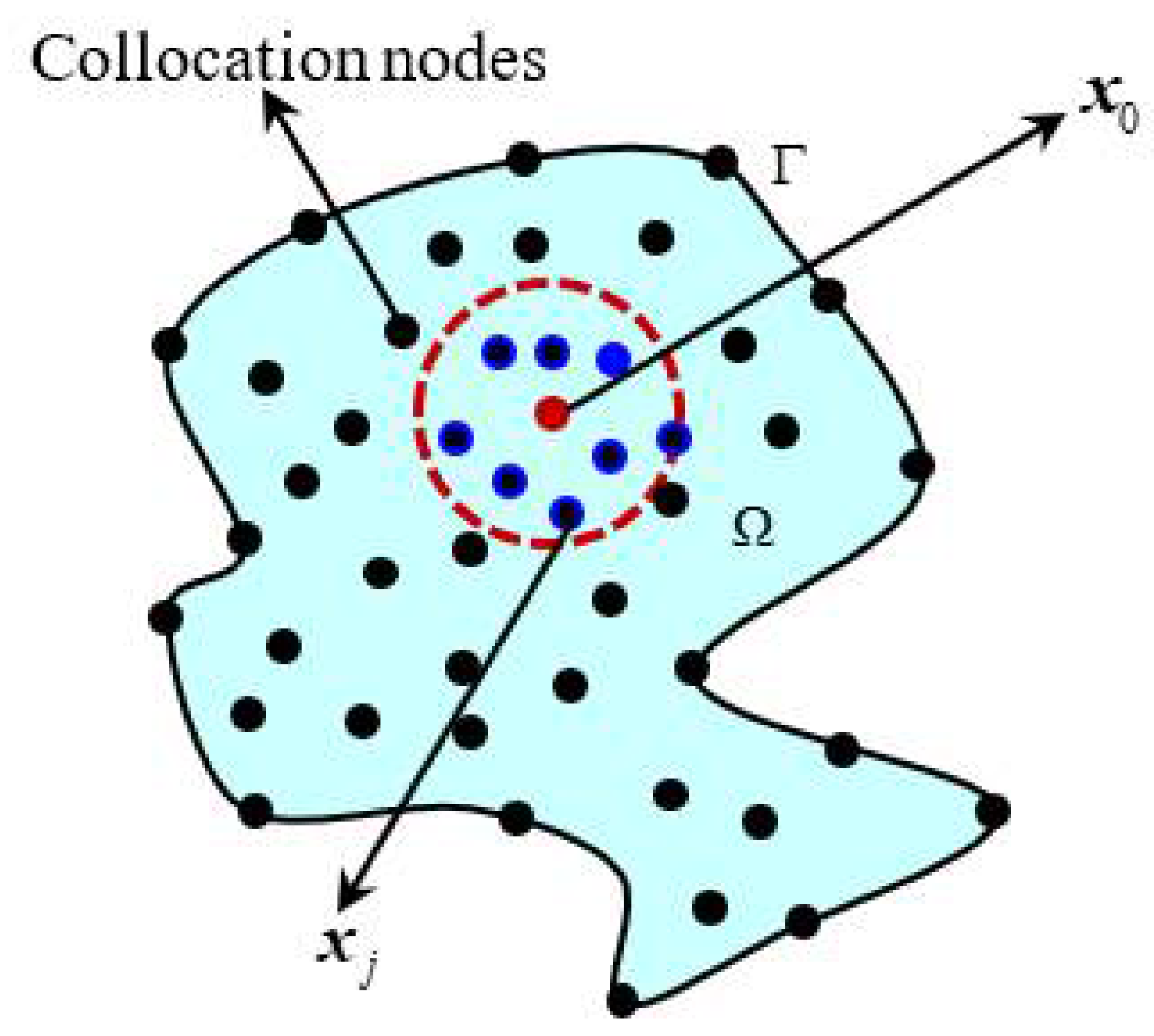
For the GFDM, some collocation nodes are first distributed in the computational domain $\mathsf{\Omega }$ and its boundary Γ. A supporting domain called a star for each node ${\mathit{x}}_0=(x_0,y_0)$ is defined by collecting $\mathit{m}$ nearest nodes ${\mathit{x}}_j=(x_j,y_j)(j=1,2,\dots ,m)$ as shown in Figure 1. In the star, ${\mathit{x}}_0$ and ${\mathit{x}}_j(j=1,2,\dots ,m)$ are respectively named as the central node and the supporting nodes. This distance criterion is the simplest way of star selection. However, it should be noted that distorted (ill-conditioned) stars may be formed based on this distance criterion, particularly for cases with very irregular distributions of collocation nodes. To overcome the above drawback, the “cross” and the “Voronoi neighbours” criterions discussed in Refs. [55,56] can be used to form more reasonable stars.

Figure 1. A star of collocation node ${\mathit{x}}_0$.

To conveniently derive the system of algebraic equations, the $H_j(j=0,1,\dots ,m)$ are employed to denote the values of hydraulic head at nodes ${\mathit{x}}_j(j=0,1,\dots ,m)$ in the star of central node ${\mathit{x}}_0$. Based on Taylor series expansions, $H_j$ can be given as

$$H_j=H_0+a_j\frac{\partial H_0}{\partial x}+b_j\frac{\partial H_0}{\partial y}+\frac{1}{2}\left(a_j^2\frac{{\partial }^2{H}_0}{\partial x^2}+b_j^2\frac{{\partial }^2{H}_0}{\partial y^2}\right)+a_j{b}_j\frac{{\partial }^2{H}_0}{\partial x\partial y}+\dots \dots ,\hspace{1em}j=1,2,\dots ,m,$$

(7)

with

$$a_j=x_j-x_0,\mathrm{and}{b}_j=y_j-y_0.$$

(8)

By truncating the expansion (7) after second-order derivatives of hydraulic head $H$, we can define a residual function $R(H)$ as the following:

$$R(H)={{\displaystyle \sum _{j=1}^m\left[\left(H_0-H_j+a_j\frac{\partial H_0}{\partial x}+b_j\frac{\partial H_0}{\partial y}+\frac{a_j^2}{2}\frac{{\partial }^2{H}_0}{\partial x^2}+\frac{b_j^2}{2}\frac{{\partial }^2{H}_0}{\partial y^2}+a_j{b}_j\frac{{\partial }^2{H}_0}{\partial x\partial y}\right){\kappa }_j\right]}}^2,$$

(9)

with the following weighting function ${\kappa }_j$ [57,58]:

$${\kappa }_j=\frac{\exp \left(-{\lambda }_j^2\right)-\exp \left(-{\lambda }_m^2\right)}{1-\exp \left(-{\lambda }_m^2\right)},\hspace{1em}j=1,2,\dots ,m,$$

(10)

in which ${\lambda }_j=\left|{\mathit{x}}_j-{\mathit{x}}_0\right|$, and ${\lambda }_m=\max \left\{{\lambda }_j,j=1,2,\dots ,m\right\}$. It should be noted that the weighting function in the GFDM should be a monotonic decreasing function of ${\lambda }_j$. Because the Taylor series approximation becomes more accurate when the distance ${\lambda }_j$ is smaller, which should have a higher weight ${\kappa }_j$ in residual function $R(H)$ of Equation (9). Some other weighting functions can be found in [53,59].

A vector ${\mathit{P}}_H$ is defined by the following:

$${\mathit{P}}_H={\left[\frac{\partial H_0}{\partial x},\frac{\partial H_0}{\partial y},\frac{{\partial }^2{H}_0}{\partial x^2},\frac{{\partial }^2{H}_0}{\partial y^2},\frac{{\partial }^2{H}_0}{\partial x\partial y}\right]}^T$$

(11)

Minimizing the residual function $R(H)$ with respect to each element in the vector ${\mathit{P}}_H$, i.e.,

$$\frac{\partial R(H)}{\partial \left\{\frac{\partial H_0}{\partial x}\right\}}=0,\frac{\partial R(H)}{\partial \left\{\frac{\partial H_0}{\partial y}\right\}}=0,\frac{\partial R(H)}{\partial \left\{\frac{{\partial }^2{H}_0}{\partial x^2}\right\}}=0,\frac{\partial R(H)}{\partial \left\{\frac{{\partial }^2{H}_0}{\partial y^2}\right\}}=0,\frac{\partial R(H)}{\partial \left\{\frac{{\partial }^2{H}_0}{\partial x\partial y}\right\}}=0,$$

(12)

we can have a system of linear equations as the following:

$$\mathit{A}{\mathit{P}}_H=\mathit{b},$$

(13)

with the following:

$$\mathit{A}={\displaystyle \sum _{j=1}^{m}diag\left({\mathit{E}}_1^{(j)}\right)\coprod diag\left({\mathit{E}}_2^{(j)}\right)},$$

(14)

$$\mathit{b}=\mathit{B}\mathit{H}={\left(-{\displaystyle \sum _{j=1}^m{\kappa }_j{\mathit{E}}_2^{(j)}},{\kappa }_1{\mathit{E}}_2^{(1)},{\kappa }_2{\mathit{E}}_2^{(2)},\cdots ,{\kappa }_m{\mathit{E}}_2^{(m)}\right)}_{5\times (m+1)}{\left(\begin{array}{l}{H}_0\\ H_1\\ H_2\\ ⋮\\ H_m\end{array}\right)}_{(m+1)\times 1},$$

(15)

where $\coprod$ is a $5\times 5$ square matrix that all elements are one, $diag\left({\mathit{E}}_1^{(j)}\right)$ and $diag\left({\mathit{E}}_2^{(j)}\right)$ are both diagonal matrices with their diagonal elements as the following:

$${\mathit{E}}_1^{(j)}={\kappa }_j{\left[\begin{array}{ccccc}{a}_j& b_j& a_j^2& b_j^2& a_j{b}_j\end{array}\right]}^T,\mathrm{and}{\mathit{E}}_2^{(j)}=\frac{{\kappa }_j}{2}{\left[\begin{array}{ccccc}2a_j& 2b_j& a_j^2& b_j^2& 2a_j{b}_j\end{array}\right]}^T,$$

(16)

and $\mathit{H}={\left[H_0,H_1,H_2,\dots ,H_m\right]}^T$.

With the help of Equation (13) and Equation (15), the vector ${\mathit{P}}_H$ can be formulated as the following:

$${\mathit{P}}_H={\mathit{A}}^{-1}\mathit{B}{\left[H_0,H_1,H_2,\dots ,H_m\right]}^T.$$

(17)

As a result, all the first- and second-order derivatives of hydraulic head $H$ at central node ${\mathit{x}}_0$ are expressed as the linear combinations of values $H_j(j=0,1,\dots ,m)$. By substituting the corresponding second-order derivatives of Equation (17) into Equation (6), we can easily recast Equation (6) as the following:

$${\displaystyle \sum _{j=0}^m{\alpha }_j{H}_j}=Q,$$

(18)

where ${\alpha }_j(j=0,1,\dots ,m)$ and $Q$ are obviously known and can be determined by Equations (6) and (17). For each collocation node excepting that of satisfying boundary condition (2), one equation can be obtained by using the above similar derivation. It should be noted that $H_0=g(x_0,y_0,t_{i+1})$ is directly used as one equation for collocation nodes of satisfying boundary condition (2). Finally, by using the GFDM, the spatial equation with the corresponding boundary conditions has been transformed into a system of linearly algebraic equations with a sparse matrix. The values of hydraulic head $H$ at all collocation nodes can be calculated once this system is solved.

In addition, we consider a case with a nonlinear volumetric flow rate in the following numerical example 4 to further verify the proposed approach. Through a similar derivation process, a nonlinear system of algebraic equations is established and solved by using “fsolve” function of MATLAB.

4. Numerical Examples

In this section, four numerical examples with square and complicated domains are given to test the accuracy and stability of the proposed method. To preferably estimate the precision of numerical results, two different error definitions are provided as the following [60,61]:

$$\mathrm{Global}\mathrm{error}=\sqrt{{\displaystyle \sum _{i=1}^N{({\overline{H}}_i-H_i)}^2}}/\sqrt{{\displaystyle \sum _{i=1}^N{H}_i{}^2}},$$

(19)

$$\mathrm{Max}\mathrm{error}=\underset{1\le i\le N}{\max }\left\{\frac{\left|{\overline{H}}_i-H_i\right|}{\left|H_i\right|}\right\}$$

(20)

in which $N$ denotes the number of collocation nodes, $H_i$ and ${\overline{H}}_i$ represents the exact and numerical results of hydraulic head at the i-th node. Unless otherwise specified, the number of supporting nodes in a star is set to $m=12$ in all numerical examples.

4.1. Example 1: Hydraulic Head Distribution in a Square Domain

As the first numerical example, we consider the distribution of hydraulic heads in a unit square domain with its central point $(0.5,0.5)$. The specific aquifer storativity is $u_s=1$, and the hydraulic conductivities are $T_x=1$ and $T_y=3$. The volumetric flow rate $W$ is given as the following:

$$W(x,y,t)=\sin \left(0.5\pi x\right)\sin \left(0.5\pi y\right)\left({\pi }^2\sin t+\cos t\right).$$

(21)

The Dirichlet boundary condition $H(x,y,t)=0$ is imposed on the boundaries $x=0,\mathrm{and}y=0$. The Neumann boundary condition $\frac{\partial H(x,y,t)}{\partial \mathit{n}}=0$ is applied to the boundaries $x=1,\mathrm{and}y=1$. The initial condition is $H(x,y,0)=0$. Based on these, the exact solution can be determined as the following:

$$H(x,y,t)=\sin (0.5\pi x)\sin (0.5\pi y)\sin t.$$

(22)

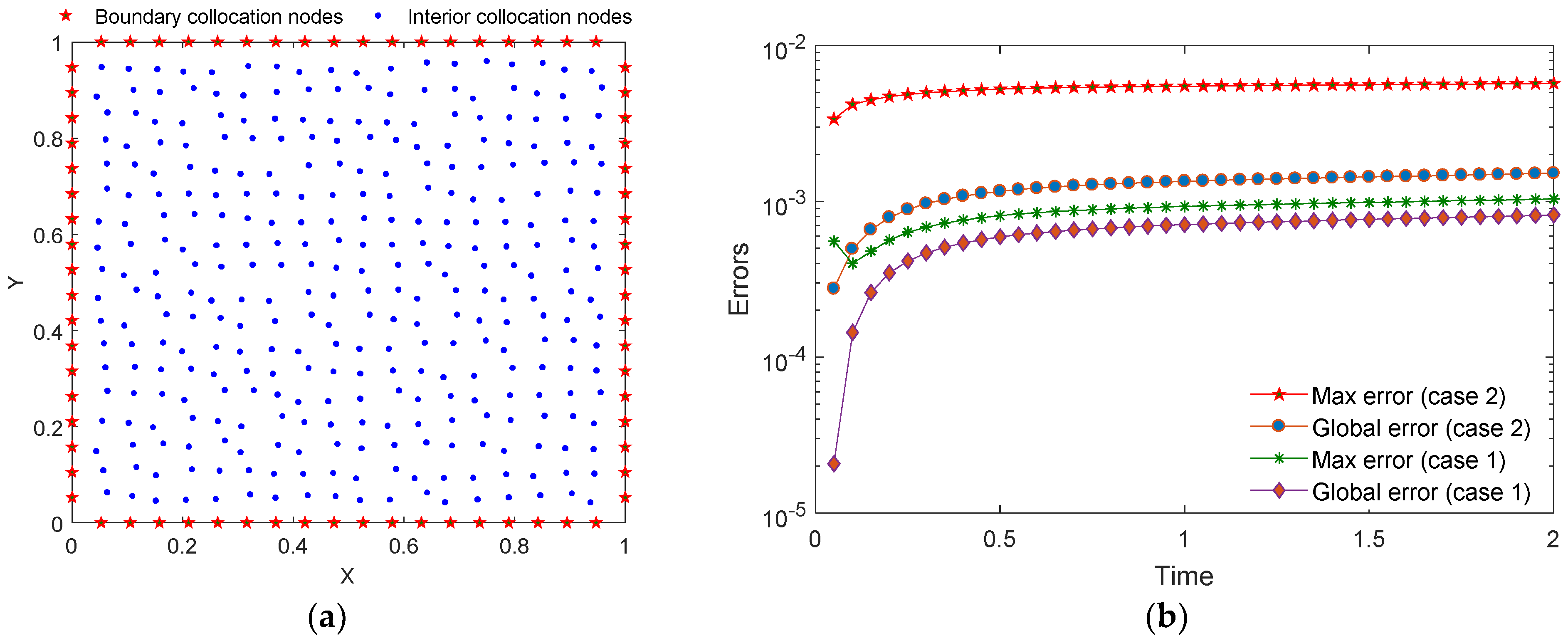
In the numerical simulation, the final time is set to $T_f=2$, and the time step size is $\Delta t=0.05$. For the spatial discretization, 396 collocation nodes are distributed in the domain and its boundary, which have the following two different patterns: regular distribution (case 1) and irregular distribution (case 2), as shown in Figure 2a. From $t=0$ to $t=2$, the variations of global and max errors of hydraulic head $H$ calculated by the GFDM with the Crank–Nicolson scheme (CN-GFDM) are plotted in Figure 2b. As we can see from this figure, the developed method has good performance for two different collocation node distributions. We also find that errors obtained by employing the irregular distribution (case 2) are larger than those obtained by using the regular distribution (case 1).

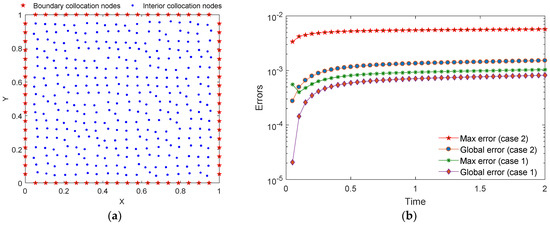
Figure 2. (a) Irregular distribution of 396 collocation nodes, (b) Global and max errors of hydraulic head $H$ from $t=0$ to $t=2$.

To investigate the convergence behavior of the CN-GFDM, the program is rerun by only changing the number of collocation nodes compared with the previous setting. Here, the distribution of nodes is regular. By using the developed method with a different number of collocation nodes (or a different mean distance of collocation nodes), Table 1 provides the max and global errors of the numerical results of the hydraulic head at time $t=2$. It can be obviously observed that the errors decay with an increasing collocation node number, which indicates the CN-GFDM has a good convergence property for this case.

Table 1. Max and global errors of hydraulic head H with different number of collocation nodes.

Number of collocation nodes	21	96	192	285	396
Mean distance of collocation nodes	$2.50\times {10}^{-1}$	$1.11\times {10}^{-1}$	$7.69\times {10}^{-2}$	$6.25\times {10}^{-2}$	$5.26\times {10}^{-2}$
Max error	$1.01\times {10}^{-2}$	$3.75\times {10}^{-3}$	$2.05\times {10}^{-3}$	$1.42\times {10}^{-3}$	$1.04\times {10}^{-3}$
Global error	$5.94\times {10}^{-3}$	$2.74\times {10}^{-3}$	$1.57\times {10}^{-3}$	$1.11\times {10}^{-3}$	$8.18\times {10}^{-4}$

4.2. Example 2: Hydraulic Head Distribution in a Heart-Shaped Domain

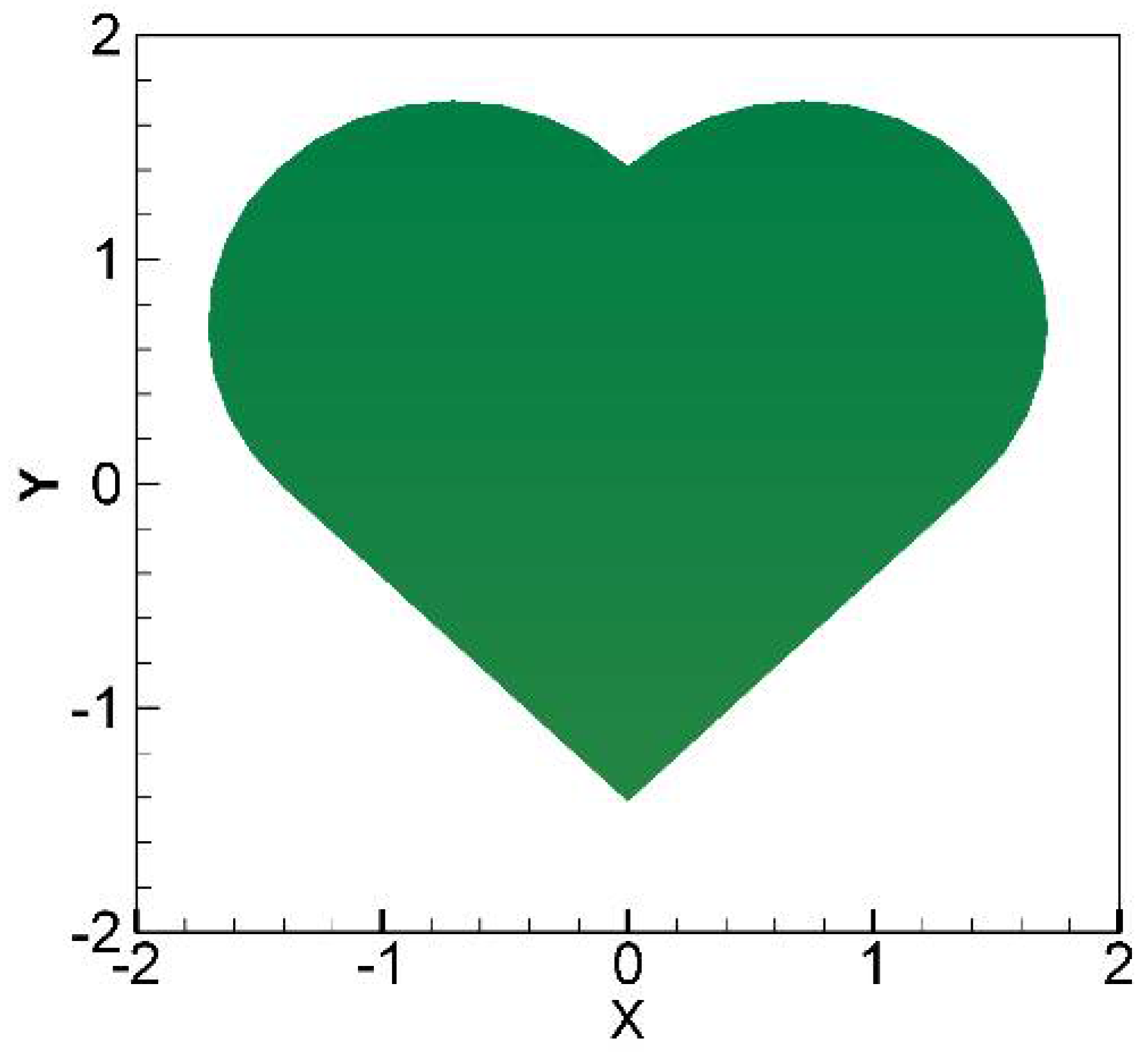
The second numerical example is a hydraulic head distribution in a heart-shaped domain, and the dimension of this domain is shown in Figure 3. The specific aquifer storativity and hydraulic conductivity are assumed to be as the following:

$$u_s=3,T_x=2T_y=2.$$

(23)

Figure 3. The dimension of a heart-shaped domain.

The volumetric flow rate is $W=0$. In this case, the Dirichlet boundary and initial conditions are imposed as the following:

$$H(x,y,t)=e^{-t}\cos x\cos y+c,\hspace{1em}(x,y)\in \Gamma ,$$

(24)

$$H(x,y,0)=\cos x\cos y+c,\hspace{1em}(x,y)\in \mathsf{\Omega },$$

(25)

where $c=0.2$. The exact solution for this example is determined as $H(x,y,t)=e^{-t}\cos x\cos y+c.$

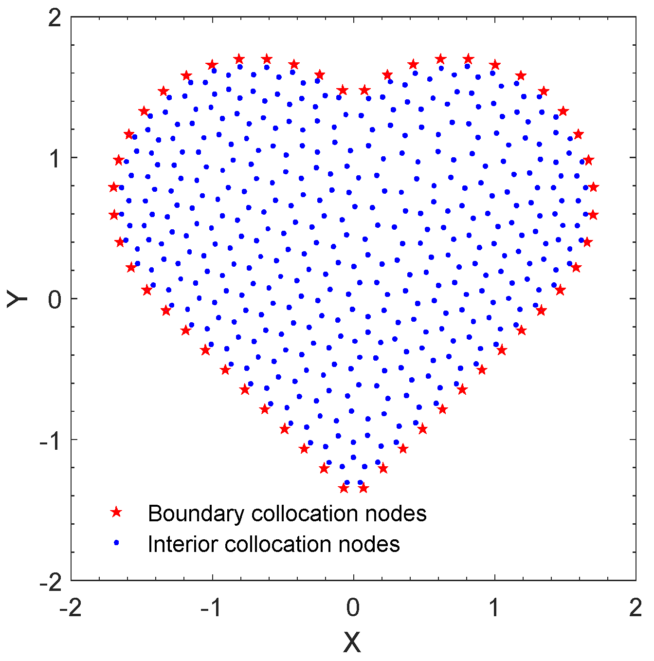
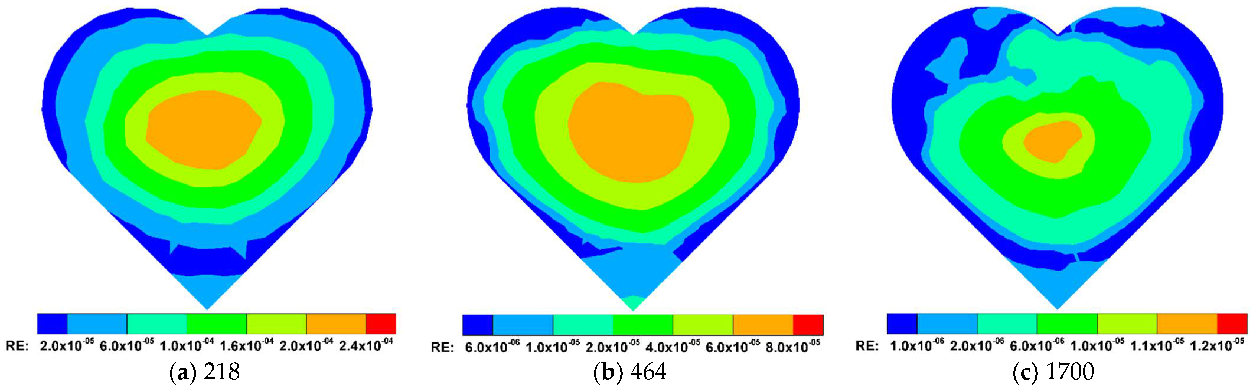
To simulate the solution from $t=0$ to $t=5$, the developed method employs 218, 464 (see Figure 4), and 1700 collocation nodes. The time step size is set to $\Delta t=0.05$. Figure 5 provides the contours of relative errors (RE) of the hydraulic head at final time $t=5$ by using these three distributions of collocation nodes. It can be found that the max relative error of numerical results in the computational domain is less than $3\times {10}^{-4}$ even only using 218 collocation nodes. Moreover, all numerical errors overall decreased with an increasing number of collocation nodes.

Figure 4. Distribution of 464 collocation nodes.

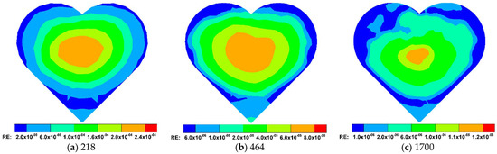
Figure 5. The contours of relative errors of hydraulic head H with three distributions of collocation nodes.

Next, we keep the above-mentioned setting and distribute 1700 collocation nodes. The mean distance of these nodes is 0.101. Table 2 lists the max and global errors of hydraulic head H at final time $t=5$, which are calculated by the CN-GFDM with different time step sizes. As we can observe, the errors decay rapidly when decreasing the time step size.

Table 2. Max and global errors of hydraulic head H with different time step size.

Time step size	0.625	0.50	0.25	0.125	0.05
Max error	$2.51\times {10}^{-3}$	$1.60\times {10}^{-3}$	$4.05\times {10}^{-4}$	$8.42\times {10}^{-5}$	$1.17\times {10}^{-5}$
Global error	$1.20\times {10}^{-3}$	$7.80\times {10}^{-4}$	$1.91\times {10}^{-4}$	$3.89\times {10}^{-5}$	$4.97\times {10}^{-6}$

Finally, we investigate the influence of supporting node number m on the precision and computational efficiency of the developed approach. The time step size is reset as $\Delta t=0.25$. Table 3 provides the variations of two kinds of errors and CPU time with different numbers of supporting nodes. As we can observe, the accuracy of numerical results obtained by the present method is relatively insensitive to the number of supporting nodes. To have a higher computing efficiency of the CN-GFDM, we should choose a relatively small number of supporting nodes when the numerical results satisfy the accuracy requirement.

Table 3. Max and global errors of hydraulic head H and CPU time with different supporting node numbers.

m	12	16	20	24	28
Max error	$4.05\times {10}^{-4}$	$3.53\times {10}^{-4}$	$3.45\times {10}^{-4}$	$3.38\times {10}^{-4}$	$3.23\times {10}^{-4}$
Global error	$1.91\times {10}^{-4}$	$1.71\times {10}^{-4}$	$1.66\times {10}^{-4}$	$1.61\times {10}^{-4}$	$1.55\times {10}^{-4}$
CPU time (s)	0.27	0.34	0.38	0.44	0.49

4.3. Example 3: Hydraulic Head Distribution in a Complicated Domain

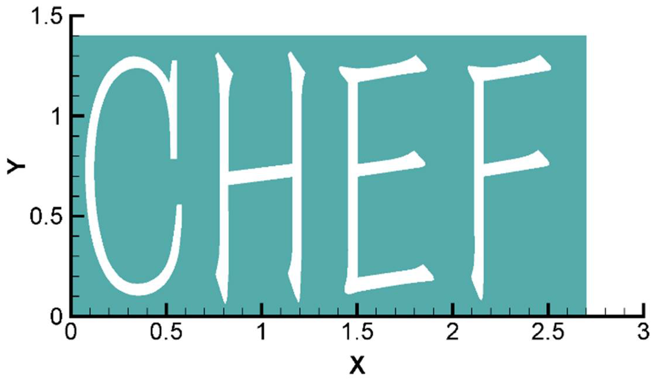
As the third numerical example, the distribution of hydraulic head in a complicated domain is considered. The dimension of this domain is $2.7\times 1.4$, as shown in Figure 6. The specific aquifer storativity is set to $u_s=0.3$, and hydraulic conductivities are assumed to be functions as the following:

$$T_x=e^{\left|x\right|},\mathrm{and}{T}_y=e^{\left|y\right|}.$$

(26)

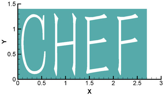
Figure 6. The dimension of a complicated domain.

The volumetric flow rate is given as the following:

$$W(x,y,t)=e^{x+y}\left[u_s\cos t-(T_x+T_y)\sin t\right]$$

(27)

The Dirichlet boundary condition is imposed as the following:

$$H(x,y,t)=e^{x+y}\sin t,\hspace{1em}(x,y)\in \Gamma ,$$

(28)

and initial condition is $H=0.$ The exact solution for this example is $H(x,y,t)=e^{x+y}\sin t.$

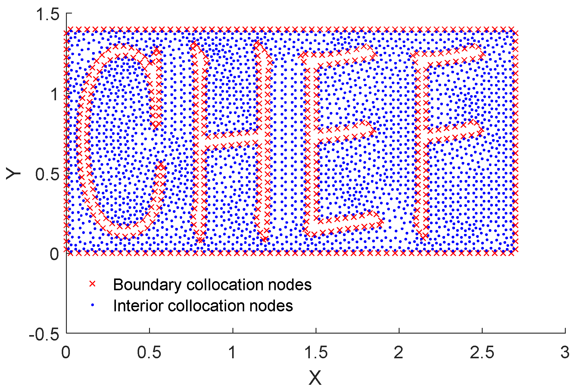
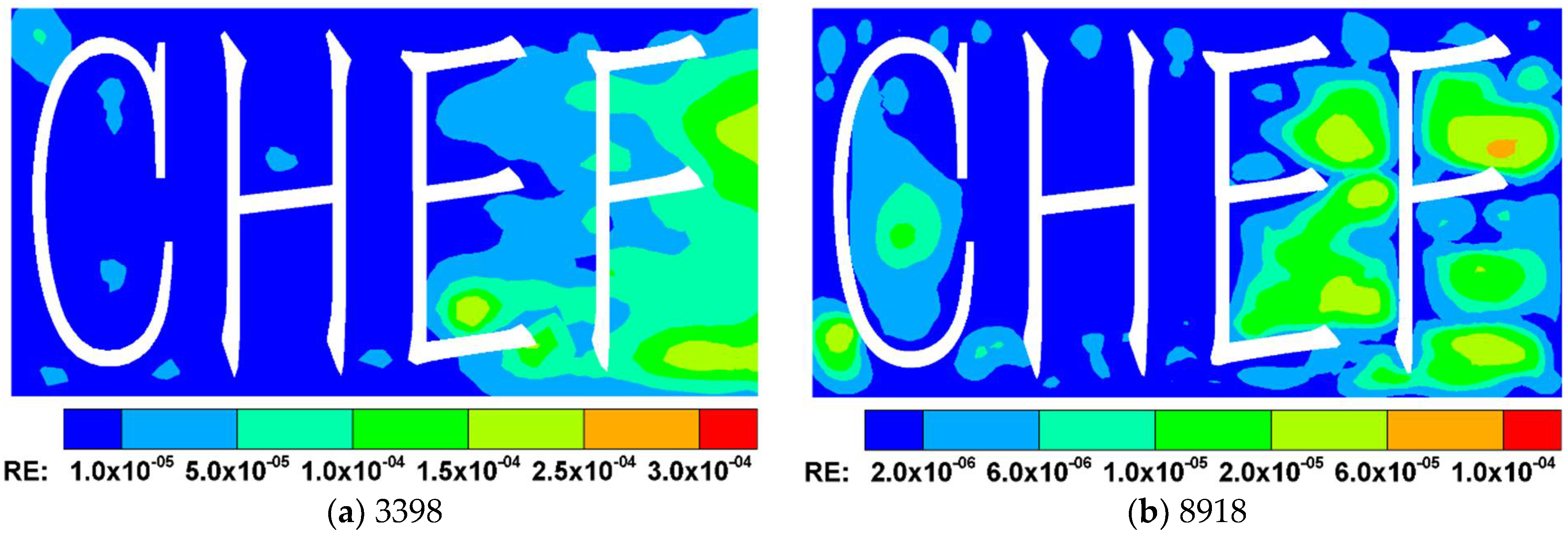
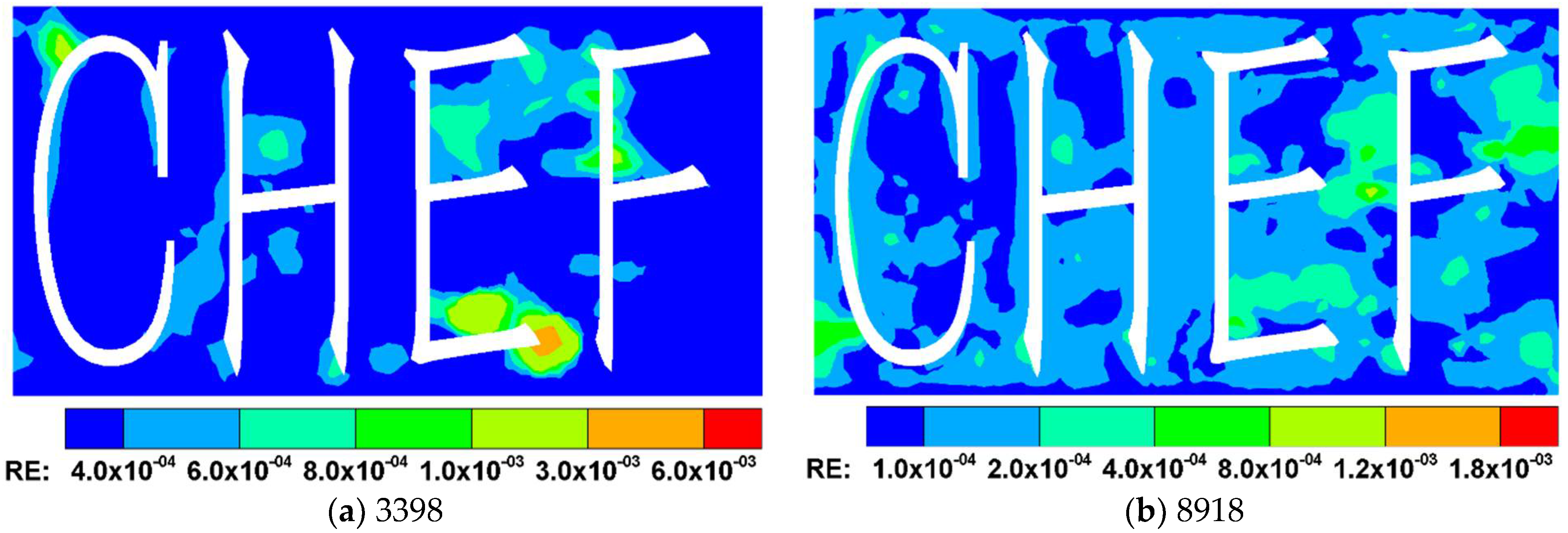
We first consider the simulation from $t=0$ to $t=5$, and set the time step size as $\Delta t=0.1$. By using the present approach with 3398 (see Figure 7) and 8918 collocation nodes, Figure 8 and Figure 9 respectively plot the contours of relative errors of hydraulic head H and its flux $\frac{\partial H}{\partial x}$ at final time $t=5$. The numerical results in these figures illustrate the availability and convergency of the developed CN-GFDM.

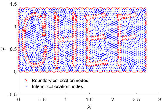
Figure 7. Distribution of 3398 collocation nodes.

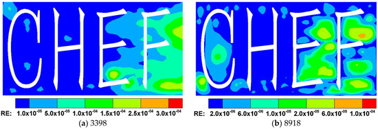
Figure 8. The contours of relative errors of hydraulic head H with two distributions of collocation nodes.

Figure 9. Relative error distributions of flux $\partial H/\partial x$ with different number of collocation nodes.

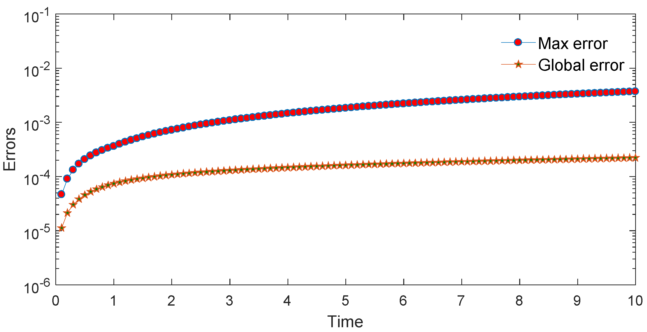
Finally, a long-time simulation of hydraulic head H from $t=0$ to $t=100$ is considered. The number of collocation nodes is 8918, and the time step size is $\Delta t=0.1$. Figure 10 shows the max and global errors of hydraulic head H, which are changed as functions of time. As we can see from this figure, the two kinds of errors both remain stable in this simulation.

Figure 10. Two types of error curves of hydraulic head H from $t=0$ to $t=100$.

4.4. Example 4: Nonlinear Hydraulic Head Distribution in a Gear Domain

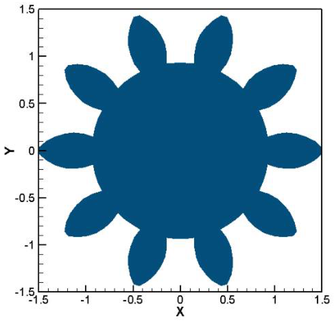
As the final numerical example, we consider the distribution of nonlinear hydraulic head in a gear domain. Figure 11 shows the dimension of the gear domain. The specific aquifer storativity is assumed to be $u_s=1200$, and hydraulic conductivities are the following:

$$T_x=x^2,\mathrm{and}{T}_y=y^2.$$

(29)

Figure 11. The dimension of a gear domain.

The volumetric flow rate is a nonlinear term given as the following:

$$W(x,y,t)=H^2(x,y,t)-{\left[\left(x^4+y^4\right)e^{\frac{t}{100}}+0.1\right]}^2$$

(30)

The Dirichlet boundary condition is imposed as the following:

$$H(x,y,t)=\left(x^4+y^4\right)e^{\frac{t}{100}}+0.1,\hspace{1em}(x,y)\in \Gamma ,$$

(31)

and initial condition is the following:

$$H(x,y,t)=x^4+y^4+0.1,\hspace{1em}(x,y)\in \mathsf{\Omega }.$$

(32)

The exact solution for this case is determined as the following:

$$H(x,y,t)=\left(x^4+y^4\right)e^{\frac{t}{100}}+0.1$$

(33)

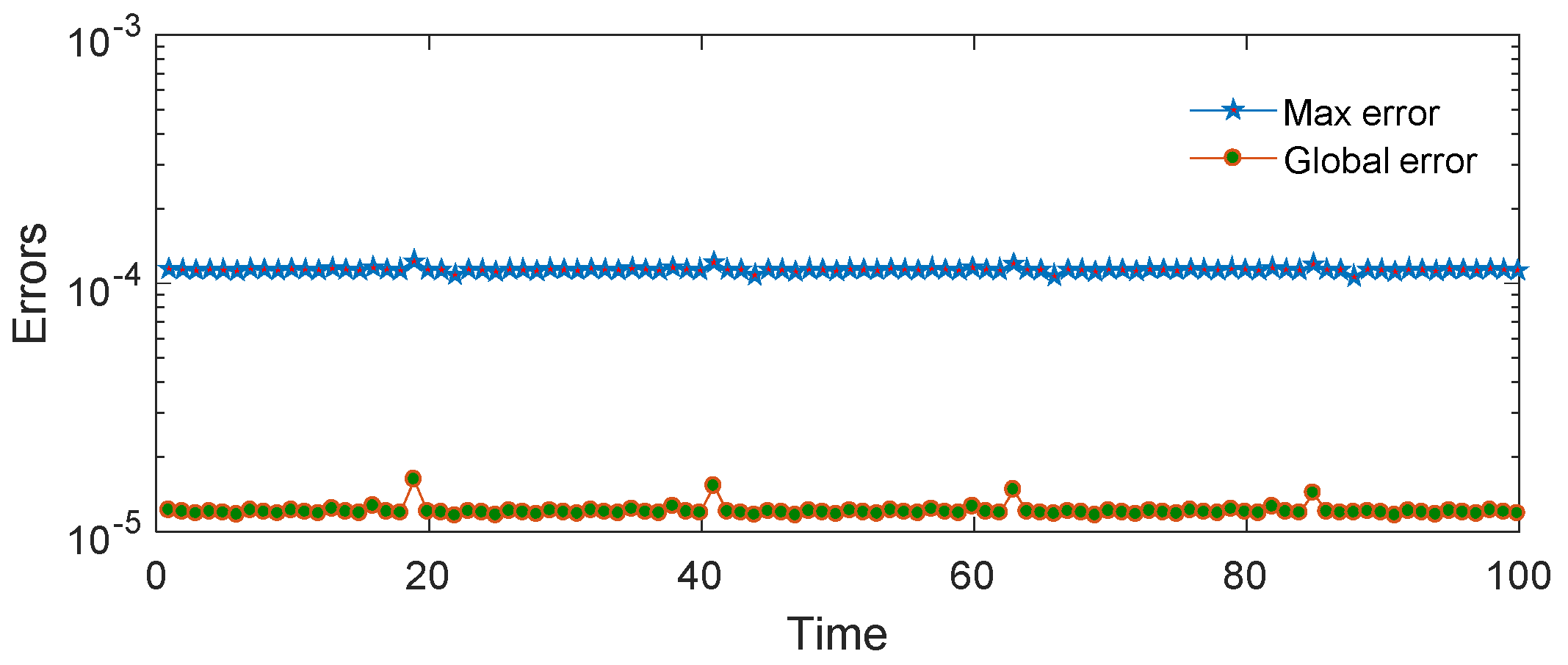
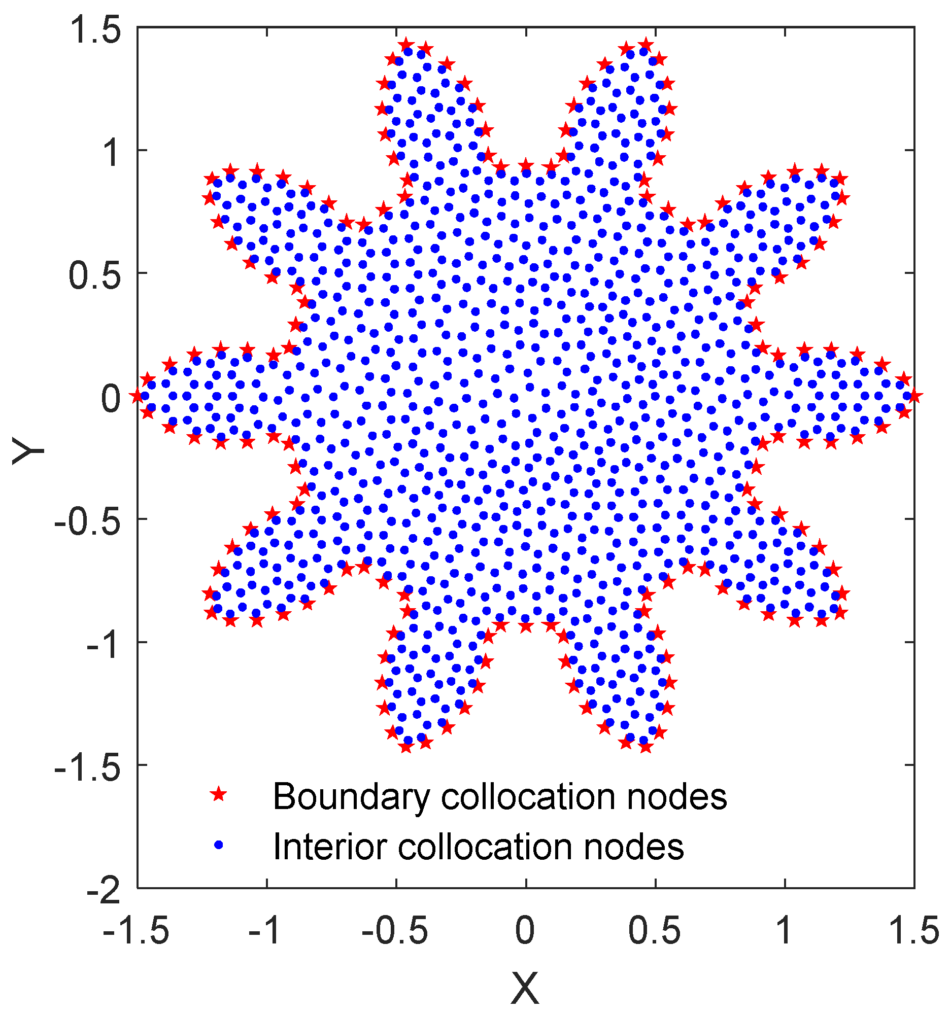
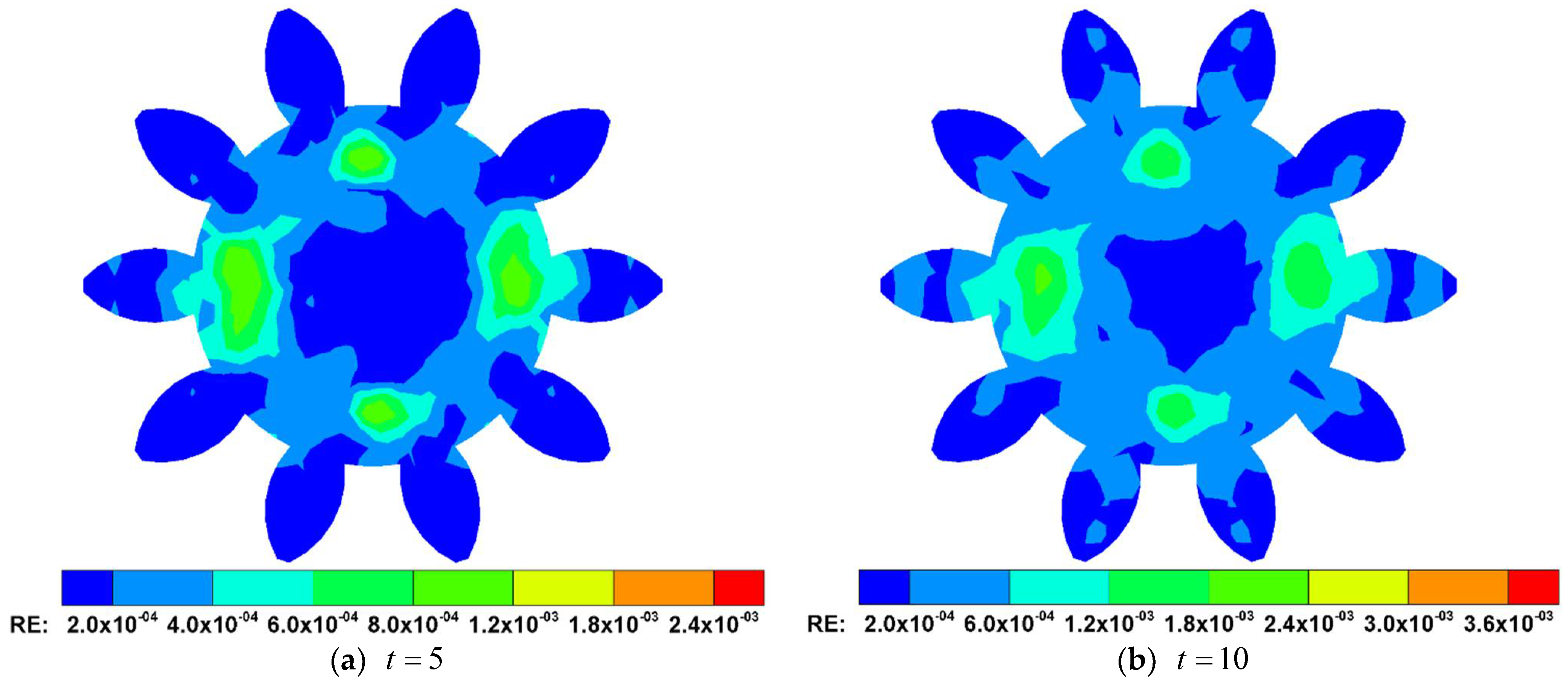
The numerical simulation for this case is run from $t=0$ to $t=10$. The time step size is set to $\Delta t=0.05$, and 1186 collocation nodes are distributed in the gear domain and its boundary as shown in Figure 12. The contours of relative errors of the hydraulic head H at $t=5$ and $t=10$ are plotted in Figure 13. As we can see from this figure, the present approach obtains the satisfied numerical results for this nonlinear case, and max relative error is less than $4\times {10}^{-3}$. Figure 14 provides the max and global errors of hydraulic head H at each time node, which illustrates that the developed CN-GFDM yields accurate numerical results as an increasing time.

Figure 12. Distribution of 1186 collocation nodes.

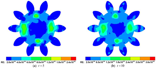
Figure 13. The contours of relative errors of hydraulic head H at $t=5$ and $t=10$.

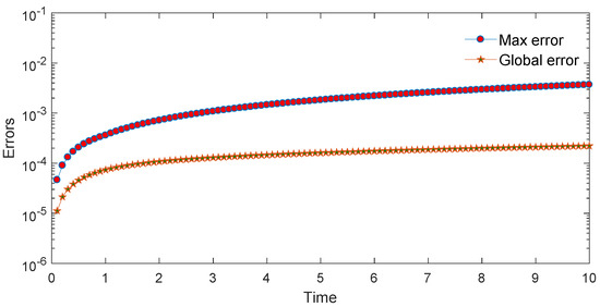
Figure 14. Two types of error curves of hydraulic head H from $t=0$ to $t=10$.

5. Concluding Remarks

To simulate the transient groundwater flow in homogeneous and anisotropic two-dimensional mediums, a hybrid localized meshless method is constructed based on the Crank–Nicolson scheme for temporal discretization and the GFDM for spatial discretization. The present approach is truly meshless and easy to program.

To fully investigate the performance of the developed method, the max and global errors of hydraulic head are both provided for numerical examples with different boundary conditions, complicated geometry domains, and several kinds of hydraulic conductivities. Numerical results indicate that the hybrid localized meshless method developed in this work obtains the satisfied accuracy and convergency in time and space.

References

- Hughes, T.J. The Finite Element Method: Linear Static and Dynamic Finite Element Analysis; Courier Corporation: Chelmsford, MA, USA, 2012. [Google Scholar]
- Chai, Y.; Li, W.; Liu, Z. Analysis of transient wave propagation dynamics using the enriched finite element method with interpolation cover functions. Appl. Math. Comput. 2022, 412, 126564. [Google Scholar] [CrossRef]
- Li, W.; Zhang, Q.; Gui, Q.; Chai, Y. A coupled FE-meshfree triangular element for acoustic radiation problems. Int. J. Comput. Methods 2021, 18, 2041002. [Google Scholar] [CrossRef]
- Qu, W.; Zhang, Y.; Liu, C.-S. Boundary stress analysis using a new regularized boundary integral equation for three-dimensional elasticity problems. Arch. Appl. Mech. 2017, 87, 1213–1226. [Google Scholar] [CrossRef]
- Gu, Y.; Zhang, C. Fracture analysis of ultra-thin coating/substrate structures with interface cracks. Int. J. Solids Struct. 2021, 225, 111074. [Google Scholar] [CrossRef]
- Zhang, X.; Liu, X.H.; Song, K.Z.; Lu, M.W. Least-squares collocation meshless method. Int. J. Numer. Methods Eng. 2001, 51, 1089–1100. [Google Scholar] [CrossRef]
- Atluri, S.N.; Shen, S. The Meshless Method; Tech Science Press: Encino, CA, USA, 2002. [Google Scholar]
- Wang, C.; Wang, F.; Gong, Y. Analysis of 2D heat conduction in nonlinear functionally graded materials using a local semi-analytical meshless method. AIMS Math. 2021, 6, 12599–12618. [Google Scholar] [CrossRef]
- Xing, Y.; Song, L.; Fan, C.-M. A generalized finite difference method for solving elasticity interface problems. Eng. Anal. Bound. Elem. 2021, 128, 105–117. [Google Scholar] [CrossRef]
- Li, X.; Dong, H. An element-free Galerkin method for the obstacle problem. Appl. Math. Lett. 2021, 112, 106724. [Google Scholar] [CrossRef]
- Xi, Q.; Fu, Z.; Wu, W.; Wang, H.; Wang, Y. A novel localized collocation solver based on Trefftz basis for potential-based inverse electromyography. Appl. Math. Comput. 2021, 390, 125604. [Google Scholar] [CrossRef]
- Tang, Z.; Fu, Z.; Chen, M.; Ling, L. A localized extrinsic collocation method for Turing pattern formations on surfaces. Appl. Math. Lett. 2021, 122, 107534. [Google Scholar] [CrossRef]
- Xi, Q.; Fu, Z.; Rabczuk, T.; Yin, D. A localized collocation scheme with fundamental solutions for long-time anomalous heat conduction analysis in functionally graded materials. Int. J. Heat Mass Transf. 2021, 180, 121778. [Google Scholar] [CrossRef]
- Lin, J.; Zhang, Y.; Reutskiy, S.; Feng, W. A novel meshless space-time backward substitution method and its application to nonhomogeneous advection-diffusion problems. Appl. Math. Comput. 2021, 398, 125964. [Google Scholar] [CrossRef]
- Qiu, L.; Hu, C.; Qin, Q.-H. A novel homogenization function method for inverse source problem of nonlinear time-fractional wave equation. Appl. Math. Lett. 2020, 109, 106554. [Google Scholar] [CrossRef]
- Sun, L.; Zhang, C.; Yu, Y. A boundary knot method for 3D time harmonic elastic wave problems. Appl. Math. Lett. 2020, 104, 106210. [Google Scholar] [CrossRef]
- Sun, L.; Chen, Z.; Zhang, S.; Chu, L. A wave based method for two-dimensional time-harmonic elastic wave propagation in anisotropic media. Appl. Math. Lett. 2021, 120, 107292. [Google Scholar] [CrossRef]
- García, Á.; Negreanu, M.; Ureña, F.; Vargas, A.M. A Note on a Meshless Method for Fractional Laplacian at Arbitrary Irregular Meshes. Mathematics 2021, 9, 2843. [Google Scholar] [CrossRef]
- Rao, X.; Zhan, W.; Zhao, H.; Xu, Y.; Liu, D.; Dai, W.; Gong, R.; Wang, F. Application of the least-square meshless method to gas-water flow simulation of complex-shape shale gas reservoirs. Eng. Anal. Bound. Elem. 2021, 129, 39–54. [Google Scholar] [CrossRef]
- Qu, W.; Fan, C.-M.; Li, X. Analysis of an augmented moving least squares approximation and the associated localized method of fundamental solutions. Comput. Math. Appl. 2020, 80, 13–30. [Google Scholar] [CrossRef]
- Gu, Y.; Fan, C.-M.; Fu, Z. Localized Method of Fundamental Solutions for Three-Dimensional Elasticity Problems: Theory. Adv. Appl. Math. Mech. 2021, 13, 1520–1534. [Google Scholar]
- Li, W. Localized method of fundamental solutions for 2D harmonic elastic wave problems. Appl. Math. Lett. 2021, 112, 106759. [Google Scholar] [CrossRef]
- Qu, W.; Gao, H.; Gu, Y. Integrating Krylov deferred correction and generalized finite difference methods for dynamic simulations of wave propagation phenomena in long-time intervals. Adv. Appl. Math. Mech. 2021, 13, 1398–1417. [Google Scholar]
- Qu, W.; He, H. A spatial–temporal GFDM with an additional condition for transient heat conduction analysis of FGMs. Appl. Math. Lett. 2020, 110, 106579. [Google Scholar] [CrossRef]
- Song, L.; Li, P.-W.; Gu, Y.; Fan, C.-M. Generalized finite difference method for solving stationary 2D and 3D Stokes equations with a mixed boundary condition. Comput. Math. Appl. 2020, 80, 1726–1743. [Google Scholar] [CrossRef]
- Shao, M.; Song, L.; Li, P.-W. A generalized finite difference method for solving Stokes interface problems. Eng. Anal. Bound. Elem. 2021, 132, 50–64. [Google Scholar] [CrossRef]
- Xing, Y.; Song, L.; Li, P.-W. A generalized finite difference method for solving biharmonic interface problems. Eng. Anal. Bound. Elem. 2022, 135, 132–144. [Google Scholar] [CrossRef]
- Li, P.-W. Space–time generalized finite difference nonlinear model for solving unsteady Burgers’ equations. Appl. Math. Lett. 2021, 114, 106896. [Google Scholar] [CrossRef]
- Li, Y.-D.; Tang, Z.-C.; Fu, Z.-J. Generalized Finite Difference Method for Plate Bending Analysis of Functionally Graded Materials. Mathematics 2020, 8, 1940. [Google Scholar] [CrossRef]
- Fan, C.-M.; Chu, C.-N.; Šarler, B.; Li, T.-H. Numerical solutions of waves-current interactions by generalized finite difference method. Eng. Anal. Bound. Elem. 2019, 100, 150–163. [Google Scholar] [CrossRef]
- Ureña, F.; Gavete, L.; Garcia, A.; Benito, J.J.; Vargas, A.M. Solving second order non-linear parabolic PDEs using generalized finite difference method (GFDM). J. Comput. Appl. Math. 2019, 354, 221–241. [Google Scholar] [CrossRef]
- Salete, E.; Vargas, A.M.; García, Á.; Negreanu, M.; Benito, J.J.; Ureña, F. Complex Ginzburg–Landau Equation with Generalized Finite Differences. Mathematics 2020, 8, 2248. [Google Scholar] [CrossRef]
- Huang, J.; Lyu, H.; Fan, C.-M.; Chen, J.-H.; Chu, C.-N.; Gu, J. Wave-Structure Interaction for a Stationary Surface-Piercing Body Based on a Novel Meshless Scheme with the Generalized Finite Difference Method. Mathematics 2020, 8, 1147. [Google Scholar] [CrossRef]
- Wang, F.; Zhao, Q.; Chen, Z.; Fan, C.-M. Localized Chebyshev collocation method for solving elliptic partial differential equations in arbitrary 2D domains. Appl. Math. Comput. 2021, 397, 125903. [Google Scholar] [CrossRef]
- Li, J.; Gu, Y.; Qin, Q.-H.; Zhang, L. The rapid assessment for three-dimensional potential model of large-scale particle system by a modified multilevel fast multipole algorithm. Comput. Math. Appl. 2021, 89, 127–138. [Google Scholar] [CrossRef]
- Li, J.; Fu, Z.; Gu, Y.; Qin, Q.-H. Recent Advances and Emerging Applications of the Singular Boundary Method for Large-Scale and High-Frequency Computational Acoustics. Adv. Appl. Math. Mech. 2021, 14, 315–343. [Google Scholar] [CrossRef]
- Li, W.; Chen, W.; Pang, G. Singular boundary method for acoustic eigenanalysis. Comput. Math. Appl. 2016, 72, 663–674. [Google Scholar] [CrossRef]
- Lin, J.; Qiu, L.; Wang, F. Localized singular boundary method for the simulation of large-scale problems of elliptic operators in complex geometries. Comput. Math. Appl. 2022, 105, 94–106. [Google Scholar] [CrossRef]
- Qiu, L.; Wang, F.; Lin, J. A meshless singular boundary method for transient heat conduction problems in layered materials. Comput. Math. Appl. 2019, 78, 3544–3562. [Google Scholar] [CrossRef]
- Wei, X.; Luo, W. 2.5D singular boundary method for acoustic wave propagation. Appl. Math. Lett. 2021, 112, 106760. [Google Scholar] [CrossRef]
- Wei, X.; Huang, A.; Sun, L. Singular boundary method for 2D and 3D heat source reconstruction. Appl. Math. Lett. 2020, 102, 106103. [Google Scholar] [CrossRef]
- Qu, W.; Chen, W. Solution of two-dimensional stokes flow problems using improved singular boundary method. Adv. Appl. Math. Mech. 2015, 7, 13–30. [Google Scholar] [CrossRef] [Green Version]
- Li, W.; Wang, F. Precorrected-FFT Accelerated Singular Boundary Method for High-Frequency Acoustic Radiation and Scattering. Mathematics 2022, 10, 238. [Google Scholar] [CrossRef]
- Wang, F.; Wang, C.; Chen, Z. Local knot method for 2D and 3D convection–diffusion–reaction equations in arbitrary domains. Appl. Math. Lett. 2020, 105, 106308. [Google Scholar] [CrossRef]
- Li, X.; Zhao, Q.; Long, K.; Zhang, H. Multi-material topology optimization of transient heat conduction structure with functional gradient constraint. Int. Commun. Heat Mass Transf. 2022, 131, 105845. [Google Scholar] [CrossRef]
- Li, X.; Li, S. On the stability of the moving least squares approximation and the element-free Galerkin method. Comput. Math. Appl. 2016, 72, 1515–1531. [Google Scholar] [CrossRef]
- Liszka, T. An interpolation method for an irregular net of nodes. Int. J. Numer. Methods Eng. 1984, 20, 1599–1612. [Google Scholar] [CrossRef]
- Liszka, T.; Orkisz, J. The finite difference method at arbitrary irregular grids and its application in applied mechanics. Comput. Struct. 1980, 11, 83–95. [Google Scholar] [CrossRef]
- Qu, W.; He, H. A GFDM with supplementary nodes for thin elastic plate bending analysis under dynamic loading. Appl. Math. Lett. 2022, 124, 107664. [Google Scholar] [CrossRef]
- Xia, H.; Gu, Y. Generalized finite difference method for electroelastic analysis of three-dimensional piezoelectric structures. Appl. Math. Lett. 2021, 117, 107084. [Google Scholar] [CrossRef]
- Qu, W. A high accuracy method for long-time evolution of acoustic wave equation. Appl. Math. Lett. 2019, 98, 135–141. [Google Scholar] [CrossRef]
- Li, P.-W.; Fu, Z.-J.; Gu, Y.; Song, L. The generalized finite difference method for the inverse Cauchy problem in two-dimensional isotropic linear elasticity. Int. J. Solids Struct. 2019, 174, 69–84. [Google Scholar] [CrossRef]
- Qu, W.; Gu, Y.; Zhang, Y.; Fan, C.M.; Zhang, C. A combined scheme of generalized finite difference method and Krylov deferred correction technique for highly accurate solution of transient heat conduction problems. Int. J. Numer. Methods Eng. 2019, 117, 63–83. [Google Scholar] [CrossRef] [Green Version]
- Chávez-Negrete, C.; Santana-Quinteros, D.; Domínguez-Mota, F. A Solution of Richards’ Equation by Generalized Finite Differences for Stationary Flow in a Dam. Mathematics 2021, 9, 1604. [Google Scholar] [CrossRef]
- Orkisz, J. Finite Difference Method; Part III. In Handbook of Computational Solid Mechanics; Kleiber, M., Ed.; Springer: Berlin/Heidelberg, Germany, 1998; pp. 336–432. [Google Scholar]
- Milewski, S. Meshless finite difference method with higher order approximation—Applications in mechanics. Arch. Comput. Methods Eng. 2012, 19, 1–49. [Google Scholar] [CrossRef]
- Belytschko, T.; Krongauz, Y.; Organ, D.; Fleming, M.; Krysl, P. Meshless methods: An overview and recent developments. Comput. Methods Appl. Mech. Eng. 1996, 139, 3–47. [Google Scholar] [CrossRef] [Green Version]
- Zhou, Y.; Qu, W.; Gu, Y.; Gao, H. A hybrid meshless method for the solution of the second order hyperbolic telegraph equation in two space dimensions. Eng. Anal. Bound. Elem. 2020, 115, 21–27. [Google Scholar] [CrossRef]
- Gavete, L.; Ureña, F.; Benito, J.J.; García, A.; Ureña, M.; Salete, E. Solving second order non-linear elliptic partial differential equations using generalized finite difference method. J. Comput. Appl. Math. 2017, 318, 378–387. [Google Scholar] [CrossRef]
- Qu, W.; Chen, W.; Gu, Y. Fast multipole accelerated singular boundary method for the 3D Helmholtz equation in low frequency regime. Comput. Math. Appl. 2015, 70, 679–690. [Google Scholar] [CrossRef]
- Qu, W.; Fan, C.-M.; Zhang, Y. Analysis of three-dimensional heat conduction in functionally graded materials by using a hybrid numerical method. Int. J. Heat Mass Transf. 2019, 145, 118771. [Google Scholar] [CrossRef]
Publisher’s Note: MDPI stays neutral with regard to jurisdictional claims in published maps and institutional affiliations. |
© 2022 by the authors. Licensee MDPI, Basel, Switzerland. This article is an open access article distributed under the terms and conditions of the Creative Commons Attribution (CC BY) license (https://creativecommons.org/licenses/by/4.0/).