A Pseudo-Spectral Fourier Collocation Method for Inhomogeneous Elliptical Inclusions with Partial Differential Equations

Abstract

Inhomogeneous elliptical inclusions with partial differential equations have aroused appreciable concern in many disciplines. In this paper, a pseudo-spectral collocation method, based on Fourier basis functions, is proposed for the numerical solutions of two- (2D) and three-dimensional (3D) inhomogeneous elliptic boundary value problems. We describe how one can improve the numerical accuracy by making some extra “reconstruction techniques” before applying the traditional Fourier series approximation. After the particular solutions have been obtained, the resulting homogeneous equation can then be calculated using various boundary-type methods, such as the method of fundamental solutions (MFS). Using Fourier basis functions, one does not need to use large matrices, making accrual computations relatively fast. Three benchmark numerical examples involving Poisson, Helmholtz, and modified-Helmholtz equations are presented to illustrate the applicability and accuracy of the proposed method.

1. Introduction

After the pioneering work of stress analyses considering elliptical region, inhomogeneous elliptical inclusions with partial differential equations have aroused appreciable concern, such as two-dimensional problems [1,2,3] and three-dimensional problems [4,5,6]. It is worth noting that the term ‘inclusions’ here refers to a medium whose properties are different from surrounding media (subdomain of the homogeneous region) inside which the eigenstrain occurs [7,8,9]. For general inhomogeneous problems, the applicability of the classical boundary element method (BEM) [10,11,12,13,14] and method of fundamental solutions (MFS) [13,15,16,17,18,19,20,21,22,23,24] depends heavily on how we evaluate the particular solution of the given problem [25,26,27,28,29,30,31,32,33,34,35,36,37,38]. One popular idea is to assume that the particular unknown solution $u_p(\mathit{x})$ can be approximated by a set of “basis functions” ${\phi }_i(\mathit{x})$:

$$u_p(\mathit{x})={\displaystyle \sum _{i=0}^N{a}_i{\phi }_i(\mathit{x})}.$$

(1)

Substituting the series (1) into the governing equation (L is the operator of the differential equation),

$$L{u}_p(\mathit{x})=f(\mathit{x}),$$

(2)

the remaining challenge is to choose the series coefficients $a_i$ so that the residual of Equation (2) can be minimized. Although many types of “basis functions” are available, a good choice for most of all applications is the Fourier series [39,40,41,42,43]. Another popular used “basis function” is the well-known Chebyshev series, which is just a Fourier cosine expansion with a change of variable [25,40,42,44,45]. Once the particular solutions have been obtained, the solution of the original problem can then be converted to a homogeneous one which can be solved by using the BEM/MFS-based methods [11,13,14,19,46,47,48,49,50,51,52,53,54,55,56,57,58,59,60,61,62,63,64].

We start in Section 2 by describing some basic mathematical theories of Fourier series, Fourier basis functions, and Fourier interpolation. We also describe how to improve numerical accuracy by making some extra “reconstruction techniques” before applying the Fourier series approximation. Section 3 is the main section, in which we describe the FCM in detail, along with how one implements it to solve the particular solutions of the given 2D and 3D boundary value problems. Next, in Section 4, a hybrid Fourier collocation method, which couples the MFS, will be presented. In Section 5, several numerical examples are presented to demonstrate the effectiveness of the present method. Finally, in Section 6, some conclusions and remarks are provided.

2. Basic Theory of Fourier Basis Functions

Let’s consider the following inhomogeneous problem:

$$Lu(\mathit{x})=f(\mathit{x}),\hspace{0.17em}\hspace{0.17em}\hspace{0.17em}\mathit{x}\in \Omega ,$$

(3)

subject to the following Dirichlet and Neumann conditions:

$$u(\mathit{x})=\overline{u}(\mathit{x})\hspace{0.17em}\hspace{0.17em}\hspace{0.17em}\hspace{0.17em}\hspace{0.17em}\mathrm{for}\hspace{0.17em}\hspace{0.17em}\mathit{x}\in {\Gamma }_D,$$

(4)

$$\frac{\partial u(\mathit{x})}{\partial \mathit{n}}=\nabla u(\mathit{x})\cdot \mathit{n}(\mathit{x})=\overline{q}(\mathit{x})\hspace{0.17em}\hspace{0.17em}\hspace{0.17em}\hspace{0.17em}\mathrm{for}\hspace{0.17em}\hspace{0.17em}\mathit{x}\in {\Gamma }_N,$$

(5)

where $\mathit{x}=(x_1,x_2)$ and $\mathit{x}=(x_1,x_2,x_3)$ for 2D and 3D problems, respectively, $\overline{u}(\mathit{x})$ and $\overline{q}(\mathit{x})$ stand for the boundary conditions specified along the boundary, $\mathit{n}(\mathit{x})$ denotes the outward unit normal vector at a boundary point $\mathit{x}$, $f(\mathit{x})$, is the inhomogeneous term. In the BEM and MFS communities, a popular way for solving a problem (3) is to split the final solution $u(\mathit{x})$ into a sum of $u_p(\mathit{x})$ (particular solution) and $u_h(\mathit{x})$ (homogeneous solution). The inhomogeneous solutions satisfy Equation (3) but do not necessarily the given boundary conditions. After $u_p(\mathit{x})$ has been calculated, the solution $u_h(\mathit{x})$ can then be obtained by solving the following problem:

$$L{u}_h(\mathit{x})=0,\hspace{0.17em}\hspace{0.17em}\hspace{0.17em}\mathit{x}\in \Omega ,$$

(6)

$$u_h(\mathit{x})=\overline{u}(\mathit{x})-u_p(\mathit{x})\hspace{0.17em}\hspace{0.17em}\hspace{0.17em}\hspace{0.17em}\hspace{0.17em}\mathrm{for}\hspace{0.17em}\hspace{0.17em}\mathit{x}\in {\Gamma }_D,$$

(7)

$$\frac{\partial u_h(\mathit{x})}{\partial n}=\overline{q}(\mathit{x})-\frac{\partial u_p(\mathit{x})}{\partial \mathit{n}}\hspace{0.17em}\hspace{0.17em}\hspace{0.17em}\hspace{0.17em}\mathrm{for}\hspace{0.17em}\hspace{0.17em}\mathit{x}\in {\Gamma }_N.$$

(8)

In our computations, the homogeneous boundary value problem (6)–(8) will be solved using the standard MFS approach, introduced in the following Section 4.

For a general one-dimensional (1D) function $f(x)$ defined on a symmetric interval $x\in$$[-L,L]$, the standard Fourier series is given explicitly as follows:

$$f(x)=a_0+{\displaystyle \sum _{n=1}^{\infty }{a}_n\cos \left(\frac{\pi nx}{L}\right)}+{\displaystyle \sum _{n=1}^{\infty }{b}_n\sin \left(\frac{\pi nx}{L}\right)},$$

(9)

where ${\left\{a_n\right\}}_{n=0}^{\infty }$ and ${\left\{b_n\right\}}_{n=1}^{\infty }$ are coefficients. Equation (9) can be expressed in the following complex form:

$$f(x)={\displaystyle \sum _{n=-\infty }^{\infty }\left(c_n{e}^{i\frac{\pi nx}{L}}\right)},$$

(10)

where $\left\{c_{-n}\right\}$ and $\left\{c_n\right\}$ are a pair of conjugate complex numbers. The relations:

$$\cos (x)=\frac{1}{2}\left(e^{ix}+e^{-ix}\right),\hspace{0.17em}\hspace{0.17em}\hspace{0.17em}\sin (x)=\frac{1}{2i}\left(e^{ix}-e^{-ix}\right).$$

(11)

indicate that (9) and (10) are completely equivalent, and we shall use whichever is convenient. In this study, the complex form Equation (10) is employed for the convenience of computer programming. For computational purposes, the function $f(x)$ is usually approximated by the following truncated Fourier series:

$$f(x)={\displaystyle \sum _{n=-N}^N\left(c_n{e}^{i\frac{\pi nx}{L}}\right)},$$

(12)

where N presents the degree of Fourier polynomials. If $f(x)$ is a known function, the Fourier coefficients ${\left\{c_n\right\}}_{n=-N}^N$ can be obtained by collocating Equation (12) on $M\ge 2N+1$ interpolation (collocation) points. This is called the “collocation” or “pseudo-spectral” method [65].

It should be noted that the Fourier series approximation (12) works best for periodic functions. It will, however, also converge for a quite arbitrary function $f(x)$ defined only on a finite interval $[-L,L]$. In such a case, we should extend $f(x)$ to $x\in \left(-\infty ,\hspace{0.17em}+\infty \right)$. For actual computations, we only care about the Fourier series expansion defined on $x\in [-L,L]$. However, such periodic extension will cause discontinuities at two extreme points $x=\pm L$, which will pollute the approximation accuracy of the Fourier series expansion. We will prove this by the following example. Suppose we take $f(x)=e^x+x^3$, $x\in [-3,\hspace{0.17em}3]$, evaluate the Fourier coefficients and sum the series (12). What do we get? We first extend the definition of $f(x)=e^x+x^3$ to $\left(-\infty ,\hspace{0.17em}+\infty \right)$. The new function is discontinuous at points $x=\pm L$($L=3$ in this example), as shown in Figure 1. We then write the truncated Fourier approximation as:

$$f(x)=e^x+x^3\approx {\displaystyle \sum _{n=-10}^{10}\left(c_n{e}^{i\frac{\pi nx}{3}}\right)},$$

(13)

where the degree of Fourier polynomials here is chosen as $N=10$. We arbitrarily choose $M=30$ interpolation points inside the interval $[-3,\hspace{0.17em}3]$, which gives $M=30$ equations, and then the Fourier coefficients ${\left\{c_n\right\}}_{n=-10}^{10}$ can be determined. After that, the function values at any points inside $[-3,\hspace{0.17em}3]$ can then be calculated by using Equation (13) again.

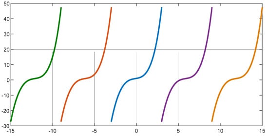
Figure 1. Periodic extensions of the function $f(x)=e^x+x^3,\hspace{0.17em}x\in [-3,\hspace{0.17em}3]$.

Figure 2a compares the exact and numerical Fourier solutions. We can observe that the discontinuity of the function at points $x=\pm 3$ has polluted the approximation with small, spurious oscillations everywhere. Near the discontinuity, there is a region where the error reaches its maximum. This fact is known as the “Gibbs Phenomenon.” Fortunately, through certain “modification” or “reconstruction,” it is possible to ameliorate some of these problems. One of the widely used techniques is to extend, smoothly, the original function $f(x)$ over $[-L,\hspace{0.17em}L]$ to $[-kL,\hspace{0.17em}kL]$ ($k>1$) so that the new function is smooth at points $x=\pm L$. From the view of mathematics, any kind of extension of $f(x)$ is fine. In actual computations, the detailed knowledge of such extension is not required since we only care about the Fourier series expansion defined on $[-L,\hspace{0.17em}L]$.

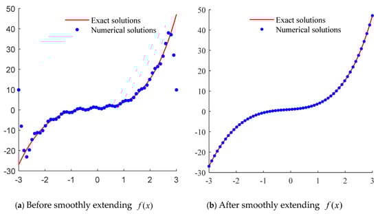
Figure 2. Comparison of the exact and Fourier-series solutions before (a) and after (b) smoothly extending the original function $f(x)$.

According to the above analysis, the original Fourier series approximation (13) can be modified as:

$$f(x)=e^x+x^3\approx {\displaystyle \sum _{n=-10}^{10}\left(c_n{e}^{i\frac{\pi nx}{3k}}\right)},$$

(14)

where $k>1$ is the so-called “period expansion coefficient,” which can be determined by the user. The source codes written in MATLAB^®2018a for this example can be found in Table 1.

Table 1. MATLAB^®2018a program for modified Fourier series approximation (14).

clc; clear;  u_exact = @(x) exp(x) + x.^3;  = 10; N_N = -N: N;  arf_arf = 2;  N_collocation = 30; L = 3;  L_extend = arf_arf *L;  x_collocation = linspace(-L, L, N_collocation)’;  = exp(i*N_N.*x_collocation*pi/L_extend);  = u_exact(x_collocation);  arf = A\B;  x_num = linspace(-L, L, 60)’;  Num = real(exp(i.*N_N.*x_num*pi/L_extend)*arf);  plot(x_num, u_exact(x_num),’r-’, x_num, Num,’bo’);

3. Fourier Collocation Method (FCM) for Particular Solutions

3.1. Two-Dimensional Problems

Suppose $F(x_1,x_2)$, $(x_1,x_2)\in [-L_1,L_1]\times [-L_2,L_2]$, is a bounded function, it can be approximated as:

$$F(x_1,x_2)={\displaystyle \sum _{m=-N_1}^{N_1}{\displaystyle \sum _{n=-N_2}^{N_2}{a}_{m,n}{e}^{i\frac{\pi m}{k{L}_1}{x}_1}{e}^{i\frac{\pi n}{k{L}_2}{x}_2}},}\hspace{0.17em}\hspace{0.17em}\hspace{0.17em}(x_1,x_2)\in [-L_1,L_1]\times [-L_2,L_2],$$

(15)

where $N_1$ and $N_2$ stand for degrees of Fourier polynomials in the $x_1$- and $x_2$-directions, respectively, $\left\{a_{m,n}\right\}$ are Fourier coefficients, and $k$ is the so-called “period expansion coefficient” as defined in Equation (14). According to the above analysis, the Fourier coefficients $\left\{a_{m,n}\right\}$ can be solved by collocating Equation (15) on $M\ge (2N_1+1)(2N_2+1)$ collocation points defined over the square $[-L_1,L_1]$$\times [-L_2,L_2]$. To guarantee the spectral convergence, it is recommended to use the Gauss–Lobatto points (the roots of Chebyshev polynomials) as the collocation points:

$${\xi }_i=\cos \left(\frac{i\pi }{n}\right),\hspace{0.17em}\hspace{0.17em}\hspace{0.17em}\hspace{0.17em}\hspace{0.17em}0\le i\le n,$$

(16)

where ${\left\{{\xi }_i\right\}}_{i=0}^n$ are the n + 1 roots of the following Chebyshev polynomial [42]:

$$T_{n+1}(x)=\cos \left[(n+1)\arccos \left(x\right)\right],\hspace{0.17em}\hspace{0.17em}\hspace{0.17em}\hspace{0.17em}x\in [-1,1].$$

(17)

As an example, Figure 3 gives the distribution of the Gauss–Lobatto points.

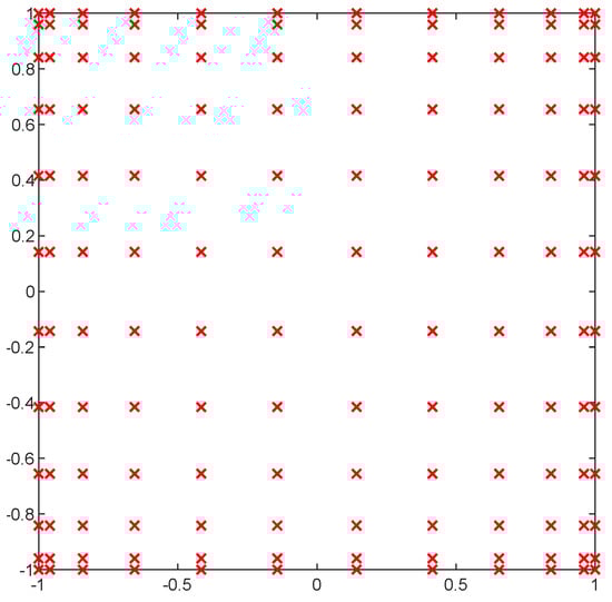
Figure 3. Distribution of Gauss–Lobatto nodes in [−1,1] × [−1,1].

For function $F(x_1,x_2)$ defined on an arbitrary domain $\left[a,b\right]\times \left[c,d\right]$, the following change of variables should be used:

$$F(x_1,x_2)={\displaystyle \sum _{m=-N_1}^{N_1}{\displaystyle \sum _{n=-N_2}^{N_2}{a}_{m,n}{e}^{i\frac{\pi m}{k{\alpha }_1}(x_1-{\beta }_1)}{e}^{i\frac{\pi n}{k{\alpha }_2}(x_2-{\beta }_2)}},}\hspace{0.17em}\hspace{0.17em}\hspace{0.17em}(x_1,x_2)\in \left[a,b\right]\times \left[c,d\right],$$

(18)

where

$${\alpha }_1=\frac{b-a}{2},\hspace{0.17em}\hspace{0.17em}\hspace{0.17em}\hspace{0.17em}\hspace{0.17em}{\beta }_1=\frac{a+b}{2},\hspace{0.17em}\hspace{0.17em}\hspace{0.17em}\hspace{0.17em}{\alpha }_2=\frac{d-c}{2},\hspace{0.17em}\hspace{0.17em}\hspace{0.17em}\hspace{0.17em}\hspace{0.17em}{\beta }_2=\frac{c+d}{2}.$$

(19)

Equation (18) is named as the shifted Fourier series expansion. Similarly, the standard Gauss–Lobatto points (collocation points) defined in $\left[-1,1\right]\times \left[-1,1\right]$, as shown in Equation (16), should be mapped into $\left[a,b\right]\times \left[c,d\right]$ as follows:

$$x_1={\alpha }_1\xi +{\beta }_1,\hspace{0.17em}\hspace{0.17em}\hspace{0.17em}{x}_2={\alpha }_2\eta +{\beta }_2,$$

(20)

where $\xi$ and $\eta$ are Gauss–Lobatto points along the $x_1$- and $x_2$-directions, respectively.

We now suppose that $F(x_1,x_2)$ be the particular solution $u_p(x_1,x_2)$ of the given inhomogeneous problem (3) defined in $\Omega$. It should be noted that, in real-world engineering applications, $\Omega$ is, in general, an arbitrary/irregular domain. Since the particular solution does not necessarily satisfy the boundary conditions, one can extend smoothly $u_p(x_1,x_2)$ from $\Omega$ to $\left[a,b\right]\times \left[c,d\right]$ containing the original domain $\Omega$, so that the shifted Fourier series expansion (18) can be used. Substituting Equation (18) into the governing Equation (3), one has:

$$L{u}_p(x_1,x_2)={\displaystyle \sum _{m=-N_1}^{N_1}{\displaystyle \sum _{n=-N_2}^{N_2}{a}_{m,n}L\left[e^{i\frac{\pi m}{k{\alpha }_1}(x_1-{\beta }_1)}{e}^{i\frac{\pi n}{k{\alpha }_2}(x_2-{\beta }_2)}\right]=f(x_1,x_2)},}\hspace{0.17em}\hspace{0.17em}\hspace{0.17em}\hspace{0.17em}(x_1,x_2)\in \left[a,b\right]\times \left[c,d\right].$$

(21)

In Equation (21), by collocating on the $M\ge (2N_1+1)(2N_2+1)$ collocation points, the unknown coefficients $\left\{a_{m,n}\right\}$ can be calculated using various minimization strategies. Finally, the particular solutions $u_p(x_1,x_2)$ can be calculated by substituting $\left\{a_{m,n}\right\}$ to the Fourier series expansion (18).

3.2. Three-Dimensional Problems

Similarly, if $F(x_1,x_2,x_3)$ is a bounded function defined in a cubic $\left[a,b\right]$$\times \left[c,d\right]$$\times \left[e,f\right]$, then it can be approximated as:

$$F(x_1,x_2,x_3)={\displaystyle \sum _{m=-N_1}^{N_1}{\displaystyle \sum _{n=-N_2}^{N_2}{\displaystyle \sum _{l=-N_3}^{N_3}{a}_{m,n,l}{e}^{i\frac{\pi m}{k{\alpha }_1}(x_1-{\beta }_1)}{e}^{i\frac{\pi n}{k{\alpha }_2}(x_2-{\beta }_2)}{e}^{i\frac{\pi l}{k{\alpha }_3}(x_3-{\beta }_3)}}},}$$

(22)

where $N_1$, $N_2$ and $N_3$ stand for degrees of Fourier polynomials in the $x_1$-, $x_2$- and $x_3$-directions, respectively, $\left\{a_{m,n,l}\right\}$ are Fourier coefficients, $k$ is the “period expansion coefficient,” ${\left\{{\alpha }_i\right\}}_{i=1}^3$ and ${\left\{{\beta }_i\right\}}_{i=1}^3$, which used to image $\left[a,b\right]$$\times \left[c,d\right]$$\times \left[e,f\right]$ to $[-L_1,L_1]$$\times [-L_2,L_2]$$\times [-L_3,L_3]$, are given as follows:

$${\alpha }_1=\frac{b-a}{2},\hspace{0.17em}\hspace{0.17em}\hspace{0.17em}\hspace{0.17em}{\beta }_1=\frac{a+b}{2},\hspace{0.17em}\hspace{0.17em}\hspace{0.17em}{\alpha }_2=\frac{d-c}{2},\hspace{0.17em}\hspace{0.17em}\hspace{0.17em}\hspace{0.17em}{\beta }_2=\frac{c+d}{2},\hspace{0.17em}\hspace{0.17em}\hspace{0.17em}{\alpha }_3=\frac{f-e}{2},\hspace{0.17em}\hspace{0.17em}\hspace{0.17em}\hspace{0.17em}{\beta }_3=\frac{e+f}{2}.$$

(23)

The standard Gauss–Lobatto points can be mapped into $\left[a,b\right]$$\times \left[c,d\right]$$\times \left[e,f\right]$ as follows:

$$x_1={\alpha }_1\xi +{\beta }_1,\hspace{0.17em}\hspace{0.17em}\hspace{0.17em}{x}_2={\alpha }_2\eta +{\beta }_2,\hspace{0.17em}\hspace{0.17em}\hspace{0.17em}{x}_3={\alpha }_3\tau +{\beta }_3.$$

(24)

where $\xi$, $\eta$ and $\tau$ are Gauss-Lobatto points along the $x_1$-, $x_2$- and $x_3$-directions, respectively.

We now suppose that $F(x_1,x_2,x_3)$ be the particular solution $u_p$ of the given problem (3), which is defined in an arbitrary/irregular 3D domain $\Omega$. Similar to the previous 2D case, we should extend smoothly $u_p(x_1,x_2,x_3)$ to a bigger cubic domain [a, b] × [c, d] × [e, f] containing the original domain $\Omega$, so that the aforementioned Fourier series expansion (22) can be used. Substituted Equation (22) into the governing Equation (3), one has:

$$L{u}_p(x_1,x_2,x_3)={\displaystyle \sum _{m=-N_1}^{N_1}{\displaystyle \sum _{n=-N_2}^{N_2}{\displaystyle \sum _{l=-N_3}^{N_3}{a}_{m,n,l}L\left[e^{i\frac{\pi m}{k{\alpha }_1}(x_1-{\beta }_1)}{e}^{i\frac{\pi n}{k{\alpha }_2}(x_2-{\beta }_2)}{e}^{i\frac{\pi l}{k{\alpha }_3}(x_3-{\beta }_3)}\right]}}=f(x_1,x_2,x_3).}$$

(25)

By collocating on the $M\ge (2N_1+1)(2N_2+1)(2N_3+1)$ collocation nodes, the coefficients $\left\{a_{m,n,l}\right\}$ can be calculated, and then the particular solutions $u_p(x_1,x_2,x_3)$ can be obtained.

4. The MFS for Homogeneous Solutions

One of the popular methods for calculating the homogeneous equation is the MFS. In the MFS approach, the homogeneous solution $u_h(\mathit{x})$ can be approximated as [47,66,67,68,69,70,71,72]:

$$u_h(\mathit{x})={\displaystyle \sum _{j=1}^{nb}{\alpha }_{j}G\left(r_j\right)},\hspace{0.17em}\hspace{0.17em}\hspace{0.17em}\hspace{0.17em}\mathit{x}\in \Omega \cup \partial \Omega ,$$

(26)

where $\mathit{x}=(x_1,x_2)$ and $\mathit{x}=(x_1,x_2,x_3)$ for 2D and 3D problems, respectively, ${\left({\alpha }_j\right)}_{j=1}^{nb}$ are the unknown coefficients, $nb$ denotes the number of source points $\left(\mathit{s}=(s_1,s_2)\hspace{0.17em}\mathrm{or}\hspace{0.17em}\mathit{s}=(s_1,s_2,s_3)\right)$ which are placed outside the computational domain, $r_j=\Vert \mathit{x}-\mathit{s}\Vert$ denotes the Euclidean distance between points $\mathit{x}$ and $\mathit{s}$, and

$$G\left(r\right)=-\frac{1}{2\pi }\log (r),$$

(27)

$$G\left(r\right)=\frac{i}{4}{H}_0^{(1)}\left(\lambda r\right),$$

(28)

$$G\left(r\right)=\frac{1}{2\pi }{K}_0^{}\left(\lambda r\right),$$

(29)

denote the fundamental solutions for 2D Poisson, Helmholtz, and modified Helmholtz equations [73], where $H_0^{(1)}$ is the Hankel function of the first kind of order zero, $K_0^{}$ stands for the modified Bessel function of the second kind of order zero, and

$$G\left(r\right)=\frac{1}{4\pi r},$$

(30)

$$G\left(r\right)=\frac{1}{4\pi r}\exp (-i\lambda r),$$

(31)

$$G\left(r\right)=\frac{1}{4\pi r}\exp (-\lambda r),$$

(32)

are fundamental solutions for 3D Poisson, Helmholtz, and modified Helmholtz equations, respectively [74]. In Equations (28), (29), (31), and (32), the parameter $\lambda$ presents the frequency of the acoustical field. The normal derivative of $u_h(\mathit{x})$ can be calculated as:

$$\frac{\partial u_h(\mathit{x})}{\partial \mathit{n}}={\displaystyle \sum _{j=1}^{nb}{\alpha }_j\left(\nabla G\left(r_j\right)\cdot \mathit{n}(\mathit{x})\right)},\hspace{0.17em}\hspace{0.17em}\hspace{0.17em}\hspace{0.17em}\mathit{x}\in \partial \Omega .$$

(33)

In the MFS, the unknown coefficients ${\left({\alpha }_j\right)}_{j=1}^{nb}$ can be calculated by collocating $M$ observation points along the boundary $\partial \Omega$ according to the specified Dirichlet (7) and Neumann (8) boundary conditions. Once all unknowns ${\left({\alpha }_j\right)}_{j=1}^{nb}$ are computed, the solution $u_h(\mathit{x})$ and its derivatives at any point inside the computational domain can be calculated. The final solution $u(\mathit{x})$ of the considered inhomogeneous problem can be calculated as $u(\mathit{x})=u_p(\mathit{x})+u_h(\mathit{x}).$ The flowchart of the present method can be found in Figure 4.

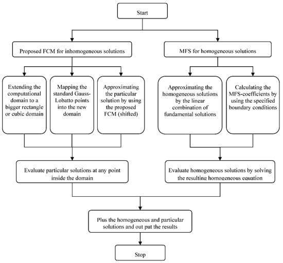
Figure 4. Flowchart for the developed FCM-MFS program.

5. Numerical Results and Discussions

Here, the stability and convergence of the present method with respect to the number of Gauss–Lobatto nodes and the degrees of Fourier polynomials are carefully investigated. In the MFS simulations, the leave-one-out cross-validation (LOOCV) method [66] is employed to determine the optimal location of the source points. In this study, all computations were implemented on a Core_i9 laptop PC with a 2.5 GHz CPU, 80 GB RAM, and 1000 GB hard drive. The platform used to write the codes is MATLAB 2021a. The following $L_2$ error norm (global error) and maximum absolute error are employed:

$$E_{Global}=\sqrt{{\displaystyle \sum _{k=1}^N{(I_{\mathrm{numerical}}^k-I_{exact}^k)}^2}}/\sqrt{{\displaystyle \sum _{k=1}^N{I}_{exact}^k{}^2}},$$

(34)

$$E_{Max}=\underset{1\le k\le N}{\max }\left|I_{\mathrm{numerical}}^k-I_{exact}^k\right|,$$

(35)

where $I_{\mathrm{numerical}}^k$ and $I_{exact}^k$ are numerical and analytical solutions, respectively.

5.1. Poisson Equation ($L={\nabla }^2$) in a 2D Multiply-Connected Domain

Firstly, let’s consider the Poisson equation with Dirichlet boundary conditions:

$${\nabla }^{2}u(x_1,x_2)=\frac{{\partial }^{2}u(x_1,x_2)}{\partial x_1^2}+\frac{{\partial }^{2}u(x_1,x_2)}{\partial x_2^2}=f(x_1,x_2),\hspace{0.17em}\hspace{0.17em}\hspace{0.17em}(x_1,x_2)\in \Omega ,$$

(36)

$$u(x_1,x_2)=\overline{u}(x_1,x_2),\hspace{0.17em}\hspace{0.17em}\hspace{0.17em}(x_1,x_2)\in \partial \Omega ,$$

(37)

where ${\nabla }^2={\partial }^2/\partial x_1^2+{\partial }^2/\partial x_2^2$ is the Laplace operator, and the inhomogeneous term $f(x_1,x_2)$ and the boundary condition $\overline{u}(x_1,x_2)$ are chosen such that satisfying the following exact solution:

$$u(x_1,x_2)=\exp (x_1+x_2)+x_1^2+x_2^2.$$

(38)

The problem considered here is a square plate with 100 circular holes (see Figure 5). For the numerical implementation, a total of $N=2080$ testing nodes are selected inside the computational domain. In the MFS, the source points are located on a circle of radius r (see Figure 6). The LOOCV method [66] is employed to determine the value of r ($r=1.986$). When using the Fourier collocation method for solving particular solutions, we use $M$$=$$(2N_1+4)$$(2N_2+4)$ Gauss–Lobatto nodes (interpolation points) to calculate the Fourier coefficients, where $N_1$ and $N_2$, as defined in Section 3, stand for degrees of Fourier polynomials along $x_1$- and $x_2$-directions, respectively.

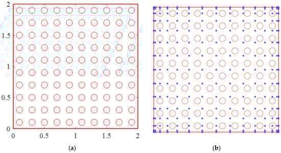
Figure 5. Geometry of the problem (a) and the distribution of the shifted Gauss–Lobatto nodes (b).

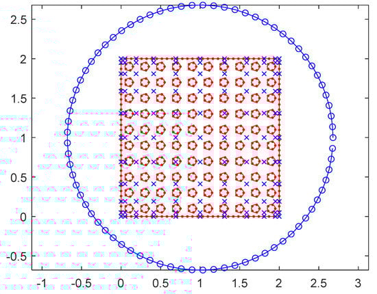
Figure 6. The profile of the multiply-connected domain, where “O”, “×”, and “•” denote the source points (MFS), shifted Gauss–Lobatto nodes and boundary points, respectively.

Firstly, we study the convergence of the present method with the degree of Fourier polynomials. For this, Table 2 shows the maximum and global errors of the calculated temperatures using the present FCM-MFS approach, as the degrees of Fourier polynomials increase from $N_1=N_2=2$ to $N_1=N_2=14$. We can observe that the calculated results are accurate and rapidly convergent as the degree of Fourier polynomials increases. We can also observe that the present method can be quite accurate even with a small degree of Fourier polynomials. The CPU times taken by the proposed method are also given in Table 2. Figure 7a,b shows the contours of errors calculated at points inside the whole domain, by using $N_1=N_2=3$ and $N_1=N_2=8$, respectively. The purpose of testing this simple problem is to verify the reliability of the proposed method for the solution of 2D inhomogeneous elliptic problems.

Table 2. Numerical results with respect to various degrees of Fourier polynomials.

Degrees of Fourier $\mathbf{Polynomials} ({\mathit{N}}_1={\mathit{N}}_2)$	Maximum Absolute $\mathbf{Error} \left({\mathit{E}}_{\mathit{M}\mathit{a}\mathit{x}}\right)$	Global Error $\left({\mathit{E}}_{\mathit{G}\mathit{l}\mathit{o}\mathit{b}\mathit{a}\mathit{l}}\right)$	CPU-Times (Second)
2	1.122 × 10−2	2.014 ×10−04	0.222
3	3.604 × 10−04	6.813 × 10−06	0.228
4	1.389 × 10−05	2.790 × 10−07	0.235
5	6.505 × 10−07	1.249 × 10−08	0.239
6	3.038 × 10−08	6.303 × 10−10	0.237
7	1.508 × 10−09	3.235 × 10−11	0.238
8	8.019 × 10−11	1.696 × 10−12	0.252
9	1.747 × 10−11	3.347 × 10−13	0.263
10	2.028 × 10−11	2.899 × 10−13	0.275
11	1.905 × 10−11	2.974 × 10−13	0.342
12	2.104 × 10−11	3.425 × 10−13	0.369
13	2.805 × 10−11	4.350 × 10−13	0.392
14	2.785 × 10−11	4.902 × 10−13	0.479

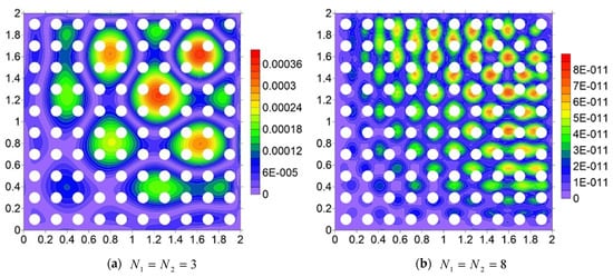
Figure 7. Relative error distribution of the calculated temperatures $u(x_1,x_2)$, where the degrees of Fourier polynomials are (a) $N_1=N_2=3$ and (b) $N_1=N_2=8$.

5.2. Helmholtz Problems ($L={\nabla }^2+{\lambda }^2$) in a 3D Dolphin-Shaped Solid

Next, let’s consider the following 3D Helmholtz equation with mixed boundary conditions:

$$\left({\nabla }^2+{\lambda }^2\right)u(x_1,x_2,x_3)=f(x_1,x_2,x_3),\hspace{0.17em}\hspace{0.17em}\hspace{0.17em}\left(x_1,x_2,x_3\right)\in \Omega ,$$

(39)

$$u(x_1,x_2,x_3)=\overline{u}(x_1,x_2,x_3),\hspace{0.17em}\hspace{0.17em}\hspace{0.17em}\left(x_1,x_2,x_3\right)\in {\Gamma }_D,$$

(40)

$$\frac{\partial u(x_1,x_2,x_3)}{\partial \mathit{n}}=\overline{q}(x_1,x_2,x_3),\hspace{0.17em}\hspace{0.17em}\hspace{0.17em}\left(x_1,x_2,x_3\right)\in {\Gamma }_N,$$

(41)

where ${\nabla }^2={\partial }^2/\partial x_1^2+{\partial }^2/\partial x_2^2+{\partial }^2/\partial x_3^2$ denotes the Laplace operator, $\lambda$ is the frequency of the acoustical field. In the above equation, the inhomogeneous term $f(x_1,x_2,x_3)$ and the boundary conditions $\overline{u}(x_1,x_2,x_3)$ $\overline{q}(x_1,x_2,x_3)$ are chosen such that satisfying the following exact solution:

$$u(x_1,x_2,x_3)=\cos (x_1+x_2+\lambda x_3).$$

(42)

Here, we consider a dolphin-shaped solid domain [42], as shown in Figure 8. The dimensions of the dolphin-shaped solid are 3.6 m (length), 1.05 m (width), and 1.36 m (height). The computational domain is extended here to the cubic $\left[-0.1,\hspace{0.17em}3.7\right]\times \left[-0.1,\hspace{0.17em}1.1\right]\times \left[-0.1,\hspace{0.17em}1.4\right]$, so that the shifted Fourier series expansion (22) can be used. A total of 7307 collocation points are selected inside the computational domain, which contains 5278 boundary nodes and 2029 interior nodes. The acoustical field is given on the left-half side of the domain $\left\{0\hspace{0.17em}\le x\le 1.8\right\}$, and the sound velocities are prescribed on the remaining boundary points. The wavenumber here is taken to be $\lambda =\sqrt{3}$. For the MFS simulations, the fictitious boundary is set to be a sphere with a radius $r=2.936$, as shown in Figure 9. When using the Fourier collocation method for solving particular solutions, we use $M$$=$$(2N_1+4)$$(2N_2+4)$$(2N_3+4)$ Gauss–Lobatto nodes to calculate the Fourier coefficients, where $N_1$, $N_2$ and $N_3$ are degrees of Fourier polynomials along $x_1$-, $x_2$- and $x_3$-directions, respectively.

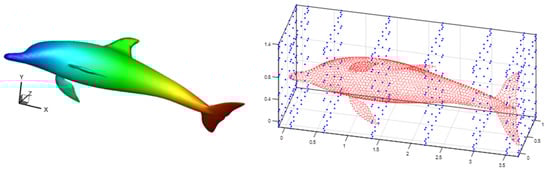
Figure 8. Geometry of the problem and the distribution of the shifted Gauss–Lobatto nodes.

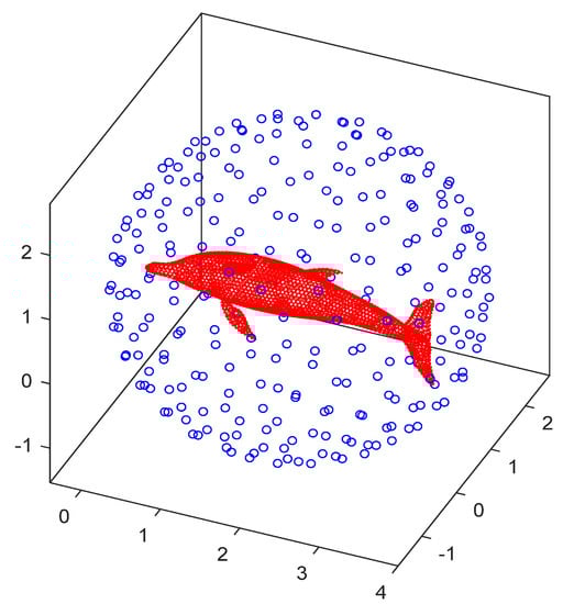
Figure 9. The profile of the dolphin-shaped solid, where “O” and “•” denote the source points (MFS) and boundary points, respectively.

Table 3 lists the maximum and global errors of the sound results calculated using the proposed FCM-MFS approach, as the degrees of Fourier polynomials increase from $N_1=N_2=N_3=1$ to $N_1=N_2=N_3=10$. These results illustrate the high accuracy and fast convergence of the present method. It can be observed that the present method can be quite accurate even with a small degree of Fourier polynomials. The CPU times are also given in Table 3. In the previous examples, we have studied the accuracy and convergence of the present method with the degrees of Fourier polynomials. Here, we investigate the effect of the wave number $\lambda D$ on the accuracy of the present FCM-MFS results, where $D=4$ denotes the maximum diameter of the domain. In our computations, the degrees of Fourier polynomials are taken to be $N_1=N_2=N_3=6$. Figure 10 illustrates the errors of sounds $u(x_1,x_2,x_3)$ and sound derivatives $\partial u(x_1,x_2,x_3)/\partial x_1$. As expected, the FCM-MFS results have been improved as the values of $\lambda D$ decrease.

Table 3. Numerical results with respect to various degrees of Fourier polynomials.

Degrees of Fourier $\mathbf{Polynomials} ({\mathit{N}}_1={\mathit{N}}_2={\mathit{N}}_3)$	Maximum Absolute $\mathbf{Error} \left({\mathit{E}}_{\mathit{M}\mathit{a}\mathit{x}}\right)$	Global Error $\left({\mathit{E}}_{\mathit{G}\mathit{l}\mathit{o}\mathit{b}\mathit{a}\mathit{l}}\right)$	CPU-Times (Second)
1	3.551 × 10−03	8.722 × 10−04	1.699
2	2.219 × 10−05	4.521 × 10−06	1.883
3	9.751 × 10−07	1.842 × 10−07	1.932
4	4.368 × 10−08	8.492 × 10−09	2.148
5	2.177 × 10−09	4.371 × 10−10	5.464
6	1.787 × 10−10	3.667 × 10−11	17.471
7	6.674 × 10−10	6.694 × 10−11	48.544
8	1.373 × 10−09	2.002 × 10−10	132.663
9	4.130 × 10−09	4.884 × 10−10	350.438
10	4.752 × 10−09	5.329 × 10−10	771.604

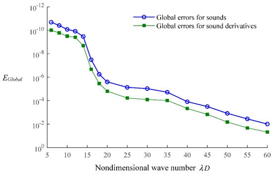
Figure 10. Relative error curves of $u$ and $\partial u/\partial x_1$ with respect to different values of non-dimensional wave number $\lambda D$.

5.3. Modified Helmholtz Problems ($L={\nabla }^2-{\lambda }^2$) in a Five Pieces Fan Blade

Finally, let’s consider the following modified Helmholtz equation:

$$\left({\nabla }^2-{\lambda }^2\right)u(x_1,x_2,x_3)=f(x_1,x_2,x_3),\hspace{0.17em}\hspace{0.17em}\hspace{0.17em}\left(x_1,x_2,x_3\right)\in \Omega ,$$

(43)

$$u(x_1,x_2,x_3)=\overline{u}(x_1,x_2,x_3),\hspace{0.17em}\hspace{0.17em}\hspace{0.17em}\left(x_1,x_2,x_3\right)\in {\Gamma }_D,$$

(44)

$$\frac{\partial u(x_1,x_2,x_3)}{\partial \mathit{n}}=\overline{q}(x_1,x_2,x_3),\hspace{0.17em}\hspace{0.17em}\hspace{0.17em}\left(x_1,x_2,x_3\right)\in {\Gamma }_N,$$

(45)

where the exact solution is chosen as:

$$u(x_1,x_2,x_3)=e^{-(x_1+x_2+\lambda x_3)}+x_1+x_2+x_3.$$

(46)

This example considers a five-piece fan blade domain [75] (see Figure 11). The dimensions of the problem are 1.5 m, 5 m and 5 m along x-, y- and z-axis coordinates, respectively. The original domain is extended to a bigger cubic $\left[-0.1,\hspace{0.17em}1.6\right]\times \left[-0.1,\hspace{0.17em}5.1\right]\times \left[-0.1,\hspace{0.17em}5.1\right]$. A total of 11,300 collocation points are selected inside the computational domain. Dirichlet boundary conditions are prescribed on the left-half side of the domain $\left\{0\hspace{0.17em}\le y\le 2.5\right\}$, and Neumann boundary conditions are given on the remaining boundary points. The wavenumber is chosen as $\lambda =\sqrt{3}$. For the MFS simulations, the fictitious boundary is set to be a sphere with a radius $r=3.695$, as shown in Figure 12. When using the Fourier collocation method for solving particular solutions, we use $M=(2N_1+4)(2N_2+4)(2N_3+4)$ Gauss–Lobatto nodes to calculate the Fourier coefficients, where $N_1$, $N_2$ and $N_3$ are degrees of Fourier polynomials along $x_1$-, $x_2$- and $x_3$-directions, respectively.

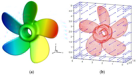
Figure 11. Geometry of the problem (a) and the distribution of the shifted Gauss–Lobatto nodes (b).

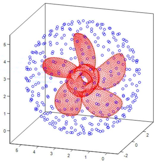
Figure 12. The profile of the five pieces fan blade domain, where “O” and “•” denote the source points (MFS) and boundary points, respectively.

Table 4 shows the maximum and global errors of the calculated FCM-MFS results as the degrees of Fourier polynomials increase from $N_1=N_2=N_3=1$ to $N_1=N_2=N_3=10$. These results indicate the high accuracy of the proposed method. Figure 13 shows the relative error curves of the calculated $u(x_1,x_2,x_3)$ and $\partial u(x_1,x_2,x_3)/\partial x_1$ as the non-dimensional wave number $\lambda D$ increases from 20 to 500, where $\lambda$ is the wavenumber and $D=5$ denotes the maximum diameter of the computational domain. In our computations, the degrees of Fourier polynomials are taken to be $N_1=N_2=N_3=6$. We can observe that the proposed FCM-MFS approach can achieve accurate results even with a relatively large value of wavenumber, for example, $\lambda D=500$.

Table 4. Numerical results with respect to various degrees of Fourier polynomials.

Degrees of Fourier $\mathbf{Polynomials} ({\mathit{N}}_1={\mathit{N}}_2={\mathit{N}}_3)$	Maximum Absolute $\mathbf{Error} \left({\mathit{E}}_{\mathit{M}\mathit{a}\mathit{x}}\right)$	Global Error $\left({\mathit{E}}_{\mathit{G}\mathit{l}\mathit{o}\mathit{b}\mathit{a}\mathit{l}}\right)$	CPU-Times (Second)
1	1.854 × 10−02	6.593 × 10−04	2.355
2	1.646 × 10−03	5.606 × 10−05	2.542
3	1.354 × 10−04	4.353 × 10−06	2.736
4	1.005 × 10−05	3.139 × 10−07	3.306
5	6.777 × 10−07	2.223 × 10−08	5.678
6	4.346 × 10−08	1.609 × 10−09	15.458
7	3.599 × 10−09	1.286 × 10−10	47.648
8	2.934 × 10−09	4.647 × 10−11	132.023
9	5.257 × 10−09	9.232 × 10−11	345.086
10	5.524 × 10−09	1.095 × 10−10	670.547

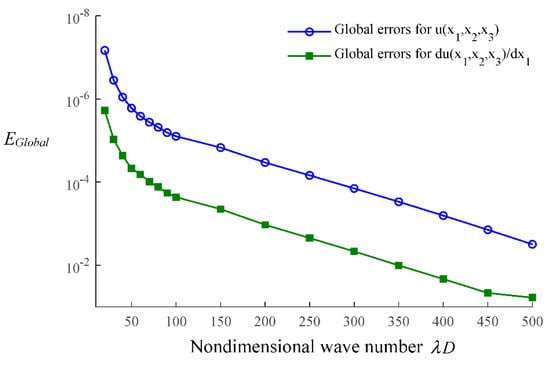
Figure 13. Relative error curves of $u$ and $\partial u/\partial x_1$ with respect to different values of non-dimensional wave number $\lambda D$.

6. Concluding Remarks

This paper presents a direct, accurate, and stable technique for the numerical solution of certain elliptic partial differential equations. In this study, an FCM technique, based on the Fourier polynomial scheme, is proposed for approximating the particular solutions of the governing equations of interest problems. To guarantee the pseudo-spectral convergence of the algorithm, the Gauss–Lobatto nodes are used as collocation points in the developed approach. After the particular solutions have been obtained, the MFS approach has been employed for solving the resulting homogeneous problem. Of course, other choices of boundary-type or localized discretization techniques are possible. Several numerical experiments illustrate that the present method is simple yet highly accurate. Though the method has been developed in the context of Poisson and Helmholtz-type equations, an extension of the method to many other problems is fairly straightforward. In addition, it is necessary to analyze and optimize the proposed method’s implementation to improve accuracy and efficiency. The analyses include convergence order of the algorithm, the parameter optimizations of the scale of the extended domain and the number of Gauss–Lobatto nodes, and new techniques of adaptive mesh refinements. The aforementioned analyses will be further investigated in future work.

References

- Zimmerman, R.W. Effective conductivity of a two-dimensional medium containing elliptical inhomogeneities. Proc. R. Soc. London Ser. A Math. Phys. Eng. Sci. 1996, 452, 1713–1727. [Google Scholar]
- Rangelov, T.V.; Manolis, G.D.; Dineva, P.S. Elastodynamic fundamental solutions for certain families of 2d inhomogeneous anisotropic domains: Basic derivations. Eur. J. Mech.—A/Solids 2005, 24, 820–836. [Google Scholar] [CrossRef]
- Markov, A.; Trofimov, A.; Sevostianov, I. A unified methodology for calculation of compliance and stiffness contribution tensors of inhomogeneities of arbitrary 2D and 3D shapes embedded in isotropic matrix—Open access software. Int. J. Eng. Sci. 2020, 157, 103390. [Google Scholar] [CrossRef]
- Gong, Y.P.; Yang, H.S.; Dong, C.Y. A novel interface integral formulation for 3D steady state thermal conduction problem for a medium with non-homogenous inclusions. Comput. Mech. 2019, 63, 181–199. [Google Scholar] [CrossRef]
- Wang, X.; Akobi, M.; Nikaeen, P.; Khattab, A.; He, T.; Li, J.; Zhang, P. Modeling and statistical understanding: The effect of carbon nanotube on mechanical properties of recycled polycaprolactone/epoxy composites. J. Appl. Polym. Sci. 2021, 138, 49886. [Google Scholar] [CrossRef]
- Wang, F.; Sohail, A.; Tang, Q.; Li, Z. Impact of Fractals Emerging from the Fitness Activities on the Retail of Smart Wearable Devices. Fractals 2021. [Google Scholar] [CrossRef]
- Hussey, B.; Nikaeen, P.; Dixon, M.D.; Akobi, M.; Khattab, A.; Cheng, L.; Wang, Z.; Li, J.; He, T.; Zhang, P. Light-weight/defect-tolerant topologically self-interlocking polymeric structure by fused deposition modeling. Compos. Part B Eng. 2020, 183, 107700. [Google Scholar] [CrossRef]
- Zhang, P.; Akobi, M.; Khattab, A. Recyclability/malleability of crack healable polymer composites by response surface methodology. Compos. Part B Eng. 2019, 168, 129–139. [Google Scholar] [CrossRef]
- Zhang, P.; Arceneaux, D.J.; Liu, Z.; Nikaeen, P.; Khattab, A.; Li, G. A crack healable syntactic foam reinforced by 3D printed healing-agent based honeycomb. Compos. Part B Eng. 2018, 151, 25–34. [Google Scholar] [CrossRef]
- Cheng, A.H.D.; Cheng, D.T. Heritage and early history of the boundary element method. Eng. Anal. Bound. Elem. 2005, 29, 268–302. [Google Scholar] [CrossRef]
- Gu, Y.; He, X.; Chen, W.; Zhang, C. Analysis of three-dimensional anisotropic heat conduction problems on thin domains using an advanced boundary element method. Comput. Math. Appl. 2018, 75, 33–44. [Google Scholar] [CrossRef]
- Gao, X.W. The radial integration method for evaluation of domain integrals with boundary-only discretization. Eng. Anal. Bound. Elem. 2002, 26, 905–916. [Google Scholar] [CrossRef]
- Gu, Y.; Fan, C.-M.; Fu, Z. Localized method of fundamental solutions for three-dimensional elasticity problems: Theory. Adv. Appl. Math. Mech. 2021, 13, 1520–1534. [Google Scholar]
- Gu, Y.; Zhang, C. Novel special crack-tip elements for interface crack analysis by an efficient boundary element method. Eng. Fract. Mech. 2020, 239, 107302. [Google Scholar] [CrossRef]
- Chen, C.S.; Cho, H.A.; Golberg, M.A. Some comments on the ill-conditioning of the method of fundamental solutions. Eng. Anal. Bound. Elem. 2006, 30, 405–410. [Google Scholar] [CrossRef]
- Cheng, A.H.D. Particular solutions of Laplacian, Helmholtz-type, and polyharmonic operators involving higher order radial basis functions. Eng. Anal. Bound. Elem. 2000, 24, 531–538. [Google Scholar] [CrossRef]
- Karageorghis, A. Efficient MFS Algorithms for Inhomogeneous Polyharmonic Problems. J. Sci. Comput. 2011, 46, 519–541. [Google Scholar] [CrossRef]
- Marin, L. Regularized method of fundamental solutions for boundary identification in two-dimensional isotropic linear elasticity. Int. J. Solids Struct. 2010, 47, 3326–3340. [Google Scholar] [CrossRef][Green Version]
- Sarler, B. Solution of potential flow problems by the modified method of fundamental solutions: Formulations with the single layer and the double layer fundamental solutions. Eng. Anal. Bound. Elem. 2009, 33, 1374–1382. [Google Scholar] [CrossRef]
- Fan, C.M.; Huang, Y.K.; Chen, C.S.; Kuo, S.R. Localized method of fundamental solutions for solving two-dimensional Laplace and biharmonic equations. Eng. Anal. Bound. Elem. 2019, 101, 188–197. [Google Scholar] [CrossRef]
- Lin, J.; Chen, W.; Wang, F. A new investigation into regularization techniques for the method of fundamental solutions. Math. Comput. Simul. 2011, 81, 1144–1152. [Google Scholar] [CrossRef]
- Liu, S.; Li, P.-W.; Fan, C.-M.; Gu, Y. Localized method of fundamental solutions for two-and three-dimensional transient convection-diffusion-reaction equations. Eng. Anal. Bound. Elem. 2021, 124, 237–244. [Google Scholar] [CrossRef]
- Gu, Y.; Golub, M.V.; Fan, C.-M. Analysis of in-plane crack problems using the localized method of fundamental solutions. Eng. Fract. Mech. 2021, 256, 107994. [Google Scholar] [CrossRef]
- Gu, Y.; Lin, J.; Wang, F. Fracture mechanics analysis of bimaterial interface cracks using an enriched method of fundamental solutions: Theory and MATLAB code. Theor. Appl. Fract. Mech. 2021, 116, 103078. [Google Scholar] [CrossRef]
- Reutskiy, S.Y.; Chen, C.S.; Tian, H.Y. A boundary meshless method using Chebyshev interpolation and trigonometric basis function for solving heat conduction problems. Int. J. Numer. Methods Eng. 2008, 74, 1621–1644. [Google Scholar] [CrossRef]
- Chen, C.S.; Fan, C.M.; Wen, P.H. The method of approximate particular solutions for solving certain partial differential equations. Numer. Methods Partial Differ. Eq. 2012, 28, 506–522. [Google Scholar] [CrossRef]
- Hon, Y.C.; Chen, W. Boundary knot method for 2D and 3D Helmholtz and convection–diffusion problems under complicated geometry. Int. J. Numer. Methods Eng. 2003, 56, 1931–1948. [Google Scholar] [CrossRef]
- Qu, W.; He, H. A spatial–temporal GFDM with an additional condition for transient heat conduction analysis of FGMs. Appl. Math. Lett. 2020, 110, 106579. [Google Scholar] [CrossRef]
- Xia, H.; Gu, Y. Generalized finite difference method for electroelastic analysis of three-dimensional piezoelectric structures. Appl. Math. Lett. 2021, 117, 107084. [Google Scholar] [CrossRef]
- Qu, W.; Fan, C.-M.; Li, X. Analysis of an augmented moving least squares approximation and the associated localized method of fundamental solutions. Comput. Math. Appl. 2020, 80, 13–30. [Google Scholar] [CrossRef]
- Wang, F.; Fan, C.-M.; Hua, Q.; Gu, Y. Localized MFS for the inverse Cauchy problems of two-dimensional Laplace and biharmonic equations. Appl. Math. Comput. 2020, 364, 124658. [Google Scholar] [CrossRef]
- Chai, Y.; You, X.; Li, W. Dispersion reduction for the wave propagation problems using a coupled “FE-Meshfree” triangular element. Int. J. Comput. Methods 2020, 17, 1950071. [Google Scholar] [CrossRef]
- Wei, X.; Huang, A.; Sun, L. Singular boundary method for 2D and 3D heat source reconstruction. Appl. Math. Lett. 2020, 102, 106103. [Google Scholar] [CrossRef]
- Qiu, L.; Hu, C.; Qin, Q.-H. A novel homogenization function method for inverse source problem of nonlinear time-fractional wave equation. Appl. Math. Lett. 2020, 109, 106554. [Google Scholar] [CrossRef]
- Qu, W.; Gao, H.; Gu, Y. Integrating Krylov deferred correction and generalized finite difference methods for dynamic simulations of wave propagation phenomena in long-time intervals. Adv. Appl. Math. Mech. 2021, 13, 1398–1417. [Google Scholar]
- Zhao, Q.; Fan, C.-M.; Wang, F.; Qu, W. Topology optimization of steady-state heat conduction structures using meshless generalized finite difference method. Eng. Anal. Bound. Elem. 2020, 119, 13–24. [Google Scholar] [CrossRef]
- Aziz, I.; Siraj-ul, I.; Šarler, B. Wavelets collocation methods for the numerical solution of elliptic BV problems. Appl. Math. Model. 2013, 37, 676–694. [Google Scholar] [CrossRef]
- Siraj-ul, I.; Aziz, I.; Ahmad, M. Numerical solution of two-dimensional elliptic PDEs with nonlocal boundary conditions. Comput. Math. Appl. 2015, 69, 180–205. [Google Scholar] [CrossRef]
- Zhang, B.; Huang, J.; Pitsianis, N.P.; Sun, X. A Fourier-series-based kernel-independent fast multipole method. J. Comput. Phys. 2011, 230, 5807–5821. [Google Scholar] [CrossRef]
- Khatri Ghimire, B.; Tian, H.Y.; Lamichhane, A.R. Numerical solutions of elliptic partial differential equations using Chebyshev polynomials. Comput. Math. Appl. 2016, 72, 1042–1054. [Google Scholar] [CrossRef]
- Chen, C.S.; Lee, S.; Huang, C.S. Derivation of particular solutions using Chebyshev polynomial based functions. Int. J. Comput. Methods 2007, 4, 15–32. [Google Scholar] [CrossRef]
- Bai, Z.-Q.; Gu, Y.; Fan, C.-M. A direct Chebyshev collocation method for the numerical solutions of three-dimensional Helmholtz-type equations. Eng. Anal. Bound. Elem. 2019, 104, 26–33. [Google Scholar] [CrossRef]
- Bialecki, B.; Karageorghis, A. Spectral Chebyshev–Fourier collocation for the Helmholtz and variable coefficient equations in a disk. J. Comput. Phys. 2008, 227, 8588–8603. [Google Scholar] [CrossRef]
- Chen, C.S.; Muleshkov, A.S.; Golberg, M.A.; Mattheij, R.M.M. A mesh-free approach to solving the axisymmetric Poisson’s equation. Numer. Methods Partial Differ. Eq. 2005, 21, 349–367. [Google Scholar] [CrossRef]
- Khatri Ghimire, B.; Li, X.; Chen, C.S.; Lamichhane, A.R. Hybrid Chebyshev polynomial scheme for solving elliptic partial differential equations. J. Comput. Appl. Math. 2020, 364, 112324. [Google Scholar] [CrossRef]
- Fu, Z.; Chen, W.; Wen, P.; Zhang, C. Singular boundary method for wave propagation analysis in periodic structures. J. Sound Vib. 2018, 425, 170–188. [Google Scholar] [CrossRef]
- Fu, Z.-J.; Xi, Q.; Chen, W.; Cheng, A.H.D. A boundary-type meshless solver for transient heat conduction analysis of slender functionally graded materials with exponential variations. Comput. Math. Appl. 2018, 76, 760–773. [Google Scholar] [CrossRef]
- Li, J.; Zhang, L.; Qin, Q.-H. A regularized method of moments for three-dimensional time-harmonic electromagnetic scattering. Appl. Math. Lett. 2021, 112, 106746. [Google Scholar] [CrossRef]
- Lin, J.; Reutskiy, S.Y.; Lu, J. A novel meshless method for fully nonlinear advection–diffusion-reaction problems to model transfer in anisotropic media. Appl. Math. Comput. 2018, 339, 459–476. [Google Scholar] [CrossRef]
- Qu, W.; Chen, W. Solution of two-dimensional stokes flow problems using improved singular boundary method. Adv. Appl. Math. Mech. 2015, 7, 13–30. [Google Scholar] [CrossRef]
- Wang, F.; Hua, Q.; Liu, C.-S. Boundary function method for inverse geometry problem in two-dimensional anisotropic heat conduction equation. Appl. Math. Lett. 2018, 84, 130–136. [Google Scholar] [CrossRef]
- Zhang, A.; Gu, Y.; Hua, Q.; Chen, W.; Zhang, C. A regularized singular boundary method for inverse Cauchy problem in three-dimensional elastostatics. Adv. Appl. Math. Mech. 2018, 10, 1459–1477. [Google Scholar] [CrossRef]
- Young, D.L.; Chen, K.H.; Lee, C.W. Novel meshless method for solving the potential problems with arbitrary domain. J. Comput. Phys. 2005, 209, 290–321. [Google Scholar] [CrossRef]
- Liu, Y.J. A new boundary meshfree method with distributed sources. Eng. Anal. Bound. Elem. 2010, 34, 914–919. [Google Scholar] [CrossRef]
- Liu, G.R.; Gu, Y.T. Boundary meshfree methods based on the boundary point interpolation methods. Eng. Anal. Bound. Elem. 2004, 28, 475–487. [Google Scholar] [CrossRef]
- Qu, W. A high accuracy method for long-time evolution of acoustic wave equation. Appl. Math. Lett. 2019, 98, 135–141. [Google Scholar] [CrossRef]
- Wang, F.; Fan, C.M.; Zhang, C.; Lin, J. A localized space-time method of fundamental solutions for diffusion and convection-diffusion problems. Adv. Appl. Math. Mech. 2020, 12, 940–958. [Google Scholar] [CrossRef]
- Wang, F.; Wang, C.; Chen, Z. Local knot method for 2D and 3D convection–diffusion–reaction equations in arbitrary domains. Appl. Math. Lett. 2020, 105, 106308. [Google Scholar] [CrossRef]
- Li, X.; Dong, H. An element-free Galerkin method for the obstacle problem. Appl. Math. Lett. 2021, 112, 106724. [Google Scholar] [CrossRef]
- Gu, Y.; Hua, Q.; Zhang, C.; He, X. The generalized finite difference method for long-time transient heat conduction in 3D anisotropic composite materials. Appl. Math. Model. 2019, 71, 316–330. [Google Scholar] [CrossRef]
- Gu, Y.; Lei, J. Fracture mechanics analysis of two-dimensional cracked thin structures (from micro- to nano-scales) by an efficient boundary element analysis. Results Appl. Math. 2021, 11, 100172. [Google Scholar] [CrossRef]
- Qu, W.; He, H. A GFDM with supplementary nodes for thin elastic plate bending analysis under dynamic loading. Appl. Math. Lett. 2022, 124, 107664. [Google Scholar] [CrossRef]
- Qiu, L.; Lin, J.; Wang, F.; Qin, Q.-H.; Liu, C.-S. A homogenization function method for inverse heat source problems in 3D functionally graded materials. Appl. Math. Model. 2021, 91, 923–933. [Google Scholar] [CrossRef]
- Song, L.; Li, P.-W.; Gu, Y.; Fan, C.M. Generalized finite difference method for solving stationary 2D and 3D Stokes equations with a mixed boundary condition. Comput. Math. Appl. 2020, 80, 1726–1743. [Google Scholar] [CrossRef]
- Boyd, J.P. The Rate of Convergence of Fourier Coefficients for Entire Functions of Infinite Order with Application to the Weideman-Cloot Sinh-Mapping for Pseudospectral Computations on an Infinite Interval. J. Comput. Phys. 1994, 110, 360–372. [Google Scholar] [CrossRef]
- Chen, C.S.; Karageorghis, A.; Li, Y. On choosing the location of the sources in the MFS. Numer. Algoritms 2016, 72, 107–130. [Google Scholar] [CrossRef]
- Karageorghis, A.; Lesnic, D.; Marin, L. The method of fundamental solutions for three-dimensional inverse geometric elasticity problems. Comput. Struct. 2016, 166, 51–59. [Google Scholar] [CrossRef]
- Alves, C.J.S.; Antunes, P.R.S. The method of fundamental solutions applied to boundary value problems on the surface of a sphere. Comput. Math. Appl. 2018, 75, 2365–2373. [Google Scholar] [CrossRef]
- Sarler, B.; Liu, Q.G. Non-singular method of fundamental solutions for two-dimensional isotropic elasticity problems. Comput. Model. Eng. Sci. 2013, 91, 235–266. [Google Scholar]
- Gu, Y.; Fan, C.-M.; Xu, R.-P. Localized method of fundamental solutions for large-scale modeling of two-dimensional elasticity problems. Appl. Math. Lett. 2019, 93, 8–14. [Google Scholar] [CrossRef]
- Ala, G.; Fasshauer, G.E.; Francomano, E.; Ganci, S.; McCourt, M.J. An augmented MFS approach for brain activity reconstruction. Math. Comput. Simul. 2017, 141, 3–15. [Google Scholar] [CrossRef]
- Fan, C.M.; Chen, C.-S.; Monroe, J. The method of fundamental solutions for solving convection-diffusion equations with variable coefficients. Adv. Appl. Math. Mech. 2009, 1, 215. [Google Scholar]
- Marin, L.; Lesnic, D. The method of fundamental solutions for the Cauchy problem associated with two-dimensional Helmholtz-type equations. Comput. Struct. 2005, 83, 267–278. [Google Scholar] [CrossRef]
- Gu, Y.; Fan, C.-M.; Qu, W.; Wang, F.; Zhang, C. Localized method of fundamental solutions for three-dimensional inhomogeneous elliptic problems: Theory and MATLAB code. Comput. Mech. 2019, 64, 1567–1588. [Google Scholar] [CrossRef]
- Gu, Y.; Fan, C.-M.; Qu, W.; Wang, F. Localized method of fundamental solutions for large-scale modelling of three-dimensional anisotropic heat conduction problems—Theory and MATLAB code. Comput. Struct. 2019, 220, 144–155. [Google Scholar] [CrossRef]
Publisher’s Note: MDPI stays neutral with regard to jurisdictional claims in published maps and institutional affiliations. |
© 2022 by the authors. Licensee MDPI, Basel, Switzerland. This article is an open access article distributed under the terms and conditions of the Creative Commons Attribution (CC BY) license (https://creativecommons.org/licenses/by/4.0/).