A Two-Step Method of Estimation for Non-Linear Mixed-Effects Models

Abstract

The main goal of this paper is to propose a two-step method for the estimation of parameters in non-linear mixed-effects models. A first-step estimate $\tilde{\theta }$ of the vector $\theta$ of parameters is obtained by solving estimation equations, with a working covariance matrix as the identity matrix. It is shown that $\tilde{\theta }$ is consistent. If, furthermore, we have an estimated covariance matrix, $\widehat{V}$, by $\tilde{\theta }$, a second-step estimator $\widehat{\theta }$ can be obtained by solving the optimal estimation equations. It is shown that $\widehat{\theta }$ maintains asymptotic optimality. We establish the consistency and asymptotic normality of the proposed estimators. Simulation results show the improvement of $\widehat{\theta }$ over $\tilde{\theta }$. Furthermore, we provide a method to estimate the variance ${\sigma }^2$ using the method of moments; we also assess the empirical performance. Finally, three real-data examples are considered.

1. Introduction

Non-linear mixed-effects models (NLMEMs) have been described in the literature, and have been used particularly in pharmacokinetics to identify sources of variability in drug concentration in the patient population [1,2]. For example, in [3] (Section 20.3), the authors discussed a toxicokinetic model, involving 15 parameters for each of the six persons in a pharmacokinetics experiment. Some methods for the estimation of fixed effects and variance components in NLMEMs have been described. The marginal density of the response variable does not have a closed-form expression, so some approximation methods have also been proposed, for example, taking a first-order Taylor expansion of the non-linear function for the conditional modes of the random effects model [4], Laplacian approximation [5], importance sampling [5,6], and Gaussian quadrature approximation [7].

Iterative estimation equations (IEEs) [8,9] have been investigated in the context of a semi-parametric regression model for longitudinal data with an unspecified covariance matrix; consistency and asymptotic efficiency have also been demonstrated [10]. However, it is time-consuming or difficult to obtain the convergence using the iterative method when the sample size is too large. Here, we improve and extend this method to the non-linear mixed-effects model.

This paper is structured as follows: In Section 2, we discuss a two-step method for estimating the parameters of non-linear mixed effects models. In Section 3, we study the asymptotic properties of the estimators. Section 4 contains details of the simulation results. In Section 5, we propose a method to estimate the variance ${\sigma }^2$. The analysis of real data is considered in Section 6. All of the technical results can be found in the Appendix A, Appendix B, Appendix C and Appendix D.

2. Estimation in a Non-linear Mixed-Effects Model

2.1. Non-linear Mixed-Effects Model

A non-linear mixed-effects (NLME) model can be expressed as follows:

$$y_{ij}=f(x_j,\beta ,{\alpha }_i)+{ϵ}_{ij},$$

where $i=1,\dots ,N;j=1,\dots ,N_i,$$y_{ij}$ is the response or observation vector for the $jth$ observation of the $ith$ individual, f is a known non-linear function, $x_j$ is the vector of covariates, $\beta$ is a population parameter vector, ${\alpha }_i$ is a vector of the unobserved latent variables that are random across subjects, and ${ϵ}_{ij}$ represents the error, independent of ${\alpha }_i$ [11]. We assume that ${\alpha }_i\sim N(0,{\tau }^2)$ and ${ϵ}_{ij}\sim N(0,{\sigma }^2)$, and that they are independent of each other [2,4,11].

Next, we describe a method for estimating the parameter $\theta =({\beta }^{{}^{\prime }},\tau {)}^{\prime }$.

2.2. Parameter Estimation

Let the responses be $y_1,y_2,\dots ,y_N$, the sample size be N, and $\mathsf{\Theta }$ be the parameter space; $\theta \in \mathsf{\Theta }$ and ${\theta }_0$ are the vectors of the true parameter.

As in the iterative estimation equation, we now use the estimation equation to estimate the parameter, as follows:

$$\begin{array}{c}\hfill F_N(\theta )=C_N^{-1}{U}_N^T(\theta )B_N(y-{\mu }_N(\theta )),\end{array}$$

(1)

where $y={(y_i)}_{1\le i\le N},U_N(\theta )=\partial {\mu }_N(\theta )/\partial \theta ,{\mu }_N(\theta )=E(y)=({\mu }_{N,1},\dots ,{\mu }_{N,N}),{\mu }_{N,i}=E(y_i),1\le i\le N,B_N=diag(B_{N,1},B_{N,2},\dots ,B_{N,N})$, $C_N=diag(c_{N,1},\dots ,c_{N,r})$ and $c_{N,k}$ is a sequence of positive constants, $1\le k\le r$, where r represents the dimensions of parameter $\theta$. The notation $U_N(\theta ),B_N,{\mu }_N(\theta )$ represents dependence on the sample size, N.

For longitudinal data, Equation (1) can be expressed as

$$\begin{array}{c}\hfill F_N(\theta )=\sum _{i=1}^N{C}_{N,i}^{-1}{U}_{N,i}^T(\theta )B_{N,i}(y_i-{\mu }_{N,i}(\theta )),\end{array}$$

(2)

where $y_i={(y_{ij})}_{1\le j\le N_i};{\mu }_{N,i}=E(y_i);B_{N,i}={(Var(y_i))}^{-1};U_{N,i}(\theta )=\partial {\mu }_{N,i}(\theta )/\partial \theta .$

Note that the generalized estimation equation (GEE) [8] corresponds to $B_{N,i}=V_i^{-1}$, $V_i=Var(y_i)$, which is the true covariance matrix, but which is usually unknown. Hence, we propose a two-step estimation method.

Let $B_{N,i}=I_{N_i}$; then, the first-step estimator $\tilde{\theta }={\tilde{\theta }}_N$ is the solution to the equation

$$\begin{array}{c}\hfill \sum _{i=1}^N{C}_{N,i}^{-1}{U}_{N,i}^T(\theta )(y_i-{\mu }_{N,i}(\theta ))=0.\end{array}$$

(3)

For the second-step estimator, we derive an estimate ${\widehat{V}}_i$ for $V_i$ using the first-step estimator ${\tilde{\theta }}_N$. Then, letting $B_i={\widehat{V}}_i^{-1}$, we use the equation $F_N(\theta )=0$ to obtain the second-step estimator ${\widehat{\theta }}_N$.

If we iterate until convergence, the iterative equation estimator (IEE) is obtained. However, it will sometimes be difficult to obtain convergence.

It is shown in the next section that, under suitable conditions, ${\tilde{\theta }}_N$ and ${\widehat{\theta }}_N$ are consistent. Furthermore, our simulations show that ${\widehat{\theta }}_N$ outperforms ${\tilde{\theta }}_N$ in terms of efficiency. Furthermore, our simulation results show that the estimated efficiency of the second-step estimate is not much different from that of the GEE method.

A challenging task during computation is solving the estimation equation, which, under such a model, typically does not have an analytic expression. We tried to solve equations with the most popular methods, such as the Newton–Raphson iterative algorithm [12], but failed. Finally, we solved the estimation equation using the non-linear Gauss–Seidel algorithm, whose convergence has been established [13].

Remark 1.

The method can only estimate the parameters involved in $\mathrm{E}(y_{ij})$. In the case of the linear mixed-effects model, the method can only estimate the fixed effects. For example, for the linear mixed-effects model $y=X\beta +Z\alpha +ϵ$, we assume the random effect $\alpha \sim N(0,R)$ and independent error ϵ, $ϵ\sim N(0,D)$. As can be seen, in order to use our method, we need to know $E(y)=X\beta$; then, we can estimate parameter β but cannot estimate the variance of random effects, R. However, under a non-linear mixed-effects model, the method can be used to estimate both the fixed effects and the variance of the random effects, as is the case for our simulation.

Remark 2.

The matrix V can occasionally be singular. In this case, we suggest using the Moore–Penrose generalized inverse of V in place of $V^{-1}$.

3. Asymptotic Properties of the Estimator

In this section, we study the consistency and asymptotic normality of first- and second-step estimators.

We assume that the first-step($B_N=I_N$) estimator $\tilde{\theta }={\tilde{\theta }}_N$ is the solution to Equation (3). Let

$${\tilde{\theta }}_N=\left\{\begin{array}{ccc}\hfill \mathrm{the}\mathrm{solution}\mathrm{of}(3),& & \mathrm{if}\mathrm{the}\mathrm{solution}(3)\mathrm{exist}\hfill \\ \hfill \mathrm{any}\theta \mathrm{in}\mathrm{the}\mathrm{parameter}\mathrm{space},& & \mathrm{if}\mathrm{the}\mathrm{solution}(3)\mathrm{does}\mathrm{not}\mathrm{exist}\hfill \end{array}\right.$$

Consider $F_N(.)$ as a map from $\mathsf{\Theta }$ to a subset of $R^r$. Let $F_N(\mathsf{\Theta })$ be the image of $\mathsf{\Theta }$ under $F_N(.)$.

For $x\in R^r$ and $A\subset R^r$, define $d(x,A)={inf}_{y\in A}|x-y|$. $A^c$ represents the complement of A.

Let ${\xi }_n$ be a sequence of non-negative random variables. We say that $lim\; inf{\xi }_n>0$ with a probability tending to one if for any $ϵ>0$ there is $\delta >0$ such that $P({\xi }_n>\delta )\ge 1-ϵ$ for large n. Note that this is equivalent to ${\xi }_n^{-1}=O_p(1)$ [14].

Theorem 1.

(i) Suppose that,

$$\begin{array}{c}\hfill F_N({\theta }_0)\to 0\end{array}$$

(4)

in probability, as $N\to \infty$.

(ii)

$$\begin{array}{c}\hfill \underset{N}{lim\; inf}d\{F_N({\theta }_0),F_N^c(\mathsf{\Theta })\}>0withprobabilitytendingtoone.\end{array}$$

(5)

Then, with a probability tending to one, the solution to (3) exists and is in Θ.

Theorem 2.

(i) Suppose that

$$F_N({\theta }_0)\to 0(4)$$

in probability, as $N\to \infty$.

(ii) Suppose for any $ϵ>0$, there is ${\mathsf{\Theta }}_0\subset \mathsf{\Theta },$ and ${\delta }_1>0,N_{{\delta }_1}>0$, such that, for large N,

$$\begin{array}{c}\hfill P(\underset{\theta \notin {\mathsf{\Theta }}_0}{inf}|F_N(\theta )-F_N({\theta }_0)|>{\delta }_1)>1-ϵ.\end{array}$$

(6)

Furthermore, suppose there are ${\delta }_2>0,N_{{\delta }_2}>0$, such that, for large N,

$$\begin{array}{c}\hfill P(\underset{\theta \in {\mathsf{\Theta }}_0,\theta \ne {\theta }_0}{inf}\frac{|F_N(\theta )-F_N({\theta }_0)|}{|\theta -{\theta }_0|}>{\delta }_2)>1-ϵ.\end{array}$$

(7)

Then, any solution to (3) is consistent.

Let $V_N$ be the covariance matrix of y.

Write ${(H_{N,j,1})}_{kl}={(c_j^{-1}\frac{{\partial }^3{\mu }_N}{\partial {\theta }_j\partial {\theta }_k\partial {\theta }_l})}^T{B}_N(y-{\mu }_N({\theta }^j)),1\le j\le r$,

${(H_{N,j,1})}_{kl},1\le j,k,l\le r$ is the $(k,l)$ element of $H_{N,j,1}$, ${\theta }^j$ lies between ${\theta }_0$ and ${\tilde{\theta }}_N(1\le j\le r)$.

${(H_{N,j,2})}_{kl}={(c_j^{-1}\frac{{\partial }^2{\mu }_N}{\partial {\theta }_j\partial {\theta }_k})}^T{B}_N(\frac{\partial {\mu }_N}{\partial {\theta }_l})+{(c_j^{-1}\frac{{\partial }^2{\mu }_N}{\partial {\theta }_j\partial {\theta }_l})}^T{B}_N(\frac{\partial {\mu }_N}{\partial {\theta }_k})+{(c_j^{-1}\frac{\partial {\mu }_N}{\partial {\theta }_j})}^T{B}_N(\frac{{\partial }^2{\mu }_N}{\partial {\theta }_k\partial {\theta }_l}),$.

$1\le j,k,l\le r{H}_{N,j,2,\epsilon }={sup}_{|\theta -{\theta }_0|\le ϵ}\parallel H_{N,j,2}\parallel ,1\le j\le r$

Theorem 3.

Suppose that

(i) The components of $\mu (\theta )$ are three-time continuously differentiable;

(ii) ${\tilde{\theta }}_N$ satisfies (3) with a probability tending to one and is consistent;

(iii) There exists $ϵ>0$ such that

$$\begin{array}{c}\hfill \frac{|{\tilde{\theta }}_N-{\theta }_0|}{{({\lambda }_{N,1}{\lambda }_{N,2})}^{1/2}}(\underset{j}{max}(H_{N,j,2,\epsilon }))\to 0\end{array}$$

in probability, where

$${\lambda }_{N,1}={\lambda }_{min}(C_N^{-1}{U}_{N0}^T{B}_N{V}_N{B}_N^T{U}_{N0}{C}_N^{-1})$$

$${\lambda }_{N,2}={\lambda }_{min}(U_{N0}^T{B}_N^T{U}_{N0}{(U_{N0}^T{B}_N{V}_N{B}_N^T{U}_{N0})}^{-1}{U}_{N0}^T{B}_N{U}_{N0})$$

$$U_{N0}=\partial {\mu }_N{(\theta )/\partial \theta |}_{\theta ={\theta }_0}$$

(iv)

$${\left[C_N^{-1}{U}_{N0}^T{B}_N{V}_N{B}_N^T{U}_{N0}{C}_N^{-1}\right]}^{-\frac{1}{2}}{F}_N({\theta }_0)\to N(0,I_r)$$

in distribution.

(v)${\left[C_N^{-1}{U}_{N0}^T{B}_N{V}_N{B}_N^T{U}_{N0}{C}_N^{-1}\right]}^{-\frac{1}{2}}{A}_{N,1}$ is bounded in probability,

${\left[C_N^{-1}{U}_{N0}^T{B}_N{V}_N{B}_N^T{U}_{N0}{C}_N^{-1}\right]}^{-\frac{1}{2}}(H_{N,j,1}({\theta }^j)),1\le j\le r$ is bounded in probability.

where ${(A_{N,1})}_{ij}={(c_i^{-1}\frac{{\partial }^2{\mu }_N}{\partial {\theta }_i\partial {\theta }_j})}^T{B}_N(y-{\mu }_N({\theta }_0))$,${(A_{N,1})}_{ij},1\le i,j\le r$ is the $(i,j)$ element of $A_{N,1}$.

Then, ${\tilde{\theta }}_N$ is asymptotically normal with mean ${\theta }_0$ and asymptotic covariance matrix

$$\begin{array}{c}\hfill {(U_{N0}^T{B}_N^T{U}_{N0})}^{-1}(U_{N0}^T{B}_N{V}_N{B}_N^T{U}_{N0}){(U_{N0}^T{B}_N{U}_{N0})}^{-1}\end{array}$$

(8)

The proofs and further details are given in the Appendix A, Appendix B, Appendix C andAppendix D.

4. Simulation

Example 1.

Consider a simple case of a non-linear mixed-effects model that can be expressed as

$$y_{ij}=e^{\beta x_j+{\alpha }_i}+{ϵ}_{ij},$$

$i=1,2,\dots ,m,j=1,2,\dots ,n_i$, where ${\alpha }_i$ and ${ϵ}_{ij}$ are independent, with ${\alpha }_i\sim N(0,{\tau }^2)$ and ${ϵ}_{ij}\sim N(0,{\sigma }^2)$. We consider ${\sigma }^2$ as a nuisance parameter whose estimation is not considered. Let ${\sigma }^2=1$; we consider the estimation of the unknown parameters β and τ.

In this model, it is easy to see that $y_i$ has the same (joint) distribution, hence, $V_i=Var(y_{ij})=V_0$ for an unspecified $n\times n$ covariance matrix, $1\le i\le m$. For the second-step estimate, $V_i$ is estimated by the method of moments (MoM) as follows:

$${\widehat{V}}_0=\frac{1}{m}\sum _{i=1}^m(y_i-{\mu }_i){(y_i-{\mu }_i)}^{{}^{\prime }}.$$

Consider a set of unbalanced data. Table 1 shows the results of a simulation in which m = 500, $n_i=2,1\le i\le 250;$ for $n_i=6,251\le i\le m$, the true parameters are $\beta =-1,\tau =1$, and $X_j,j=1,\dots ,n$ generated from N(0, 1). The results are based on 500 simulations. We find a 13.21% improvement in the second-step estimator over the first-step estimator in terms of the total mean squared error, and the second-step estimator is very close to the GEE estimator in efficiency.

Table 1. Simulation result: non-linear model.

	$\mathit{\beta }=-1$			$\mathit{\tau }=1$			Overall
Estimator	Mean	Bias	SD	Mean	Bias	SD	MSE
1st-step	−1.0006	−0.0006	0.0321	0.9891	−0.0109	0.0644	0.0053
2nd-step	−0.9993	0.0007	0.0184	0.9849	−0.0151	0.0631	0.0046
GEE	−0.9992	0.0008	0.0182	0.9961	−0.0039	0.0622	0.0042

SD, standard deviation. Overall MSE represents the mean squared error of the estimator of β + the mean squared error of the estimator of τ.

Example 2.

Consider the following non-linear mixed-effects model, an exponential model, which may be used to model changes in drug concentration. Let

$$y_{ij}={\beta }_{1}exp(-({\beta }_2+{\alpha }_i)t_j)+{ϵ}_{ij},i=1,\dots ,m; j=1,\dots ,n,$$

where ${\alpha }_i$ is the random effect with a distribution $N(0,{\tau }^2)$, and ${ϵ}_{ij}$ is the error, which is independent of ${\alpha }_i$, with distribution $N(0,{\sigma }^2)$. ${\beta }_1$ and ${\beta }_2$ are fixed parameters. $t_j$ represents the time of observation. Assuming that ${\sigma }^2>0$ is known, we estimate parameter $\theta =({\beta }_1,{\beta }_2,\tau )$.

Let $m=500$ and $n=11$, with the true parameters ${\beta }_1=2,{\beta }_2=1,\tau =1,{\sigma }^2=0.5,t_j=(1:n)/n,j=1,\dots ,n$. The results, based on 500 simulation runs, are presented in Table 2. We see an improvement of approximately 12.5% in the second-step estimator over the first-step estimator in terms of the total mean squared error. Furthermore, we see that the second-step estimate is comparable to the GEE method.

Table 2. Simulation estimation result.

	${\mathit{\beta }}_1=2$			${\mathit{\beta }}_2=1$			$\mathit{\tau }=1$			Overall
Estimator	Mean	Bias	SD	Mean	Bias	SD	Mean	Bias	SD	MSE
1st-step	1.9804	−0.0196	0.0404	0.9463	−0.0537	0.1015	0.9421	−0.0579	0.0974	0.0280
2nd-step	1.9985	−0.0015	0.0429	0.9914	−0.0086	0.1080	0.9835	−0.0165	0.1032	0.0245
GEE	1.9989	−0.0011	0.0428	0.9933	−0.0067	0.1082	0.9854	−0.0146	0.1033	0.0245

SD, standard deviation. Overall MSE represents the mean squared error of the estimator of β₁ + the mean squared error of the estimator of β₂ + the mean squared error of the estimator of τ.

5. Estimate of Variance ${\sigma }^2$

We have so far not discussed how to estimate the variance ${\sigma }^2$. Now, we propose a method to estimate this parameter and study its empirical performance.

For a non-linear mixed-effects model

$$\begin{array}{c}\hfill y_{ij}=f(x_j,\beta ,{\alpha }_i)+{ϵ}_{ij},i=1,\dots ,m; j=1,\dots ,n_i,\end{array}$$

(9)

we assume the same conditions as in Section 2.1. Let ${\alpha }_i=\tau {\xi }_i$, ${\xi }_i\sim N(0,1)$, we have

$$\begin{array}{c}\hfill E{\{y_{ij}-f(x_j,\beta ,\tau {\xi }_i)\}}^2=E({ϵ}_{ij}^2)={\sigma }^2.\end{array}$$

(10)

The summation of both sides of $(10)$ over $i=1,\dots ,m;j=1,\dots ,n_i$ leads to

$$\begin{array}{c}\hfill E\left[\sum _{i=1}^m\sum _{j=1}^{n_i}{\{y_{ij}-f(x_j,\beta ,\tau {\xi }_i)\}}^2\right]=N{\sigma }^2,\end{array}$$

(11)

where $N={\sum }_{i=1}^m{n}_i$. If ${\xi }_i,i=1,\dots ,m$ were observable, by removing the expectation sign on the left side of $(11)$, and replacing $\beta$ and $\tau$ by their available estimators, $\widehat{\beta }$ and $\widehat{\tau }$, respectively, an empirical method of moments (EMM) estimator of ${\sigma }^2$ would be obtained, that is,

$$\begin{array}{c}\hfill {\sigma }^2=\frac{1}{N}\sum _{i=1}^m\sum _{j=1}^{n_i}{\{y_{ij}-f(x_j,\widehat{\beta },\widehat{\tau }{\xi }_i)\}}^2.\end{array}$$

(12)

The difficulty is, of course, that ${\xi }_i,i=1,\dots ,m$ are unobserved. To handle this situation, we replace ${\xi }_i,i=1,\dots ,m$ on the right side of $(12)$ with their conditional expectations given y, ${\widehat{\xi }}_i$ and $i=1,\dots ,m$, respectively, that is,

$$\begin{array}{c}\hfill {\sigma }^2=\frac{1}{N}\sum _{i=1}^m\sum _{j=1}^{n_i}{\{y_{ij}-f(x_j,\widehat{\beta },\widehat{\tau }{\widehat{\xi }}_i)\}}^2.\end{array}$$

(13)

To compute the conditional expectations, we need to know the parameters, $\theta =(\beta ,\tau )$ and ${\sigma }^2$. The $\theta$ is replaced by the current estimator, $\widehat{\theta }$. As for ${\sigma }^2$, we use an idea similar to the EM algorithm. Let ${\sigma }_c^2$ be the current estimator of ${\sigma }^2$. Then, the conditional expectations are computed under $\theta$ and ${\sigma }_c^2$, denoted by ${\widehat{\xi }}_{i,\theta ,{\sigma }_c^2},1\le i\le m$. We then use

$$\begin{array}{c}\hfill {\sigma }_u^2=\frac{1}{N}\sum _{i=1}^m\sum _{j=1}^{n_i}{\{y_{ij}-f(x_j,\widehat{\beta },\widehat{\tau }{\widehat{\xi }}_{i,\theta ,{\sigma }_c^2})\}}^2\end{array}$$

(14)

to update ${\sigma }^2$, from ${\sigma }_c^2$ to ${\sigma }_u^2$. We continue until convergence, that is, when $|{\sigma }_u^2-{\sigma }_c^2|\le \delta$ (e.g., $\delta =0.001$). The final estimator, ${\sigma }_u^2$, is denoted by ${\widehat{\sigma }}^2$. The initial estimator, ${\sigma }_0^2$, is obtained by the right side of $(13)$ with ${\xi }_i=0,1\le i\le m$. We now consider an example.

Example 3.

(Example 1 Continued). In this model, we obtain

$$\begin{array}{c}\hfill {\sigma }^2=\frac{1}{N}\sum _{i=1}^m\sum _{j=1}^{n_i}{\{y_{ij}-e^{\beta x_j+\tau {\xi }_i}\}}^2.\end{array}$$

(15)

and

$$\begin{array}{c}\hfill {\widehat{\xi }}_i=E({\xi }_i|y_i)=\frac{E{\xi }_i{\prod }_{j=1}^{n_i}f(y_{ij}|{\xi }_i)}{E{\prod }_{j=1}^{n_i}f(y_{ij}|{\xi }_i)},\end{array}$$

(16)

where $f(y_{ij}|{\xi }_i)$ is the condition probability density function, and it is obvious that $y_{ij}|{\xi }_i\sim N(e^{\beta x_j+\tau {\xi }_i},{\sigma }^2)$.

The parameter $\theta =(\beta ,\tau )$ is replaced by the estimator $\widehat{\theta }$, either the first-step estimate or second-step estimate. Then, using the same simulation design as Example 1, we iterate $(15)$ and $(16)$ to obtain the estimator ${\widehat{\sigma }}^2$. Based on 500 simulation runs, we found that some solutions did not converge, so we used the converge solution to obtain the results, which are shown in Table 3. The results show that there is little difference using a different method, but the estimation result is good. We can use either the first-step estimate or second-step estimate for the next step.

Table 3. Estimate ${\sigma }^2$.

${\mathit{\sigma }}^2=1$	mean	var	mse	% of Convergence
1st-step	1.1019	0.0277	0.0380	46.247
2nd-step	1.1106	0.0398	0.0520	42.857
GEE	1.1028	0.0300	0.0405	44.794

Remark 3.

The results in Table 3 are based on the converged solutions only. An implication is that, if the solution converges one may expect a good estimate from this procedure. In our real-data analysis results, the solution converged in all cases. A topic of future work would be to improve the estimator with better convergence.

6. Real Data

6.1. Height of Girls

The data are from the Longitudinal Studies of Child Health Development project, initiated in 1929 at the Harvard School of Public Health (the full description of the project is given by Stuart and Reed, 1929 [15]), which consists of the heights of 67 girls and 67 boys aged from 7 to 18, as described in chapter 8, Demidenko (2013) [16]. Here, we only consider the data for the girls, see Figure 1; the data from the boys are similar.

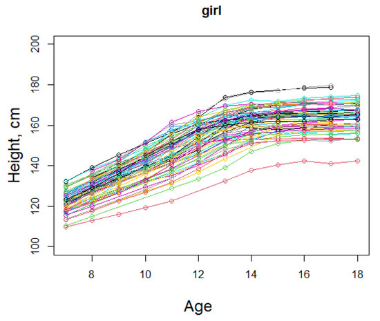
Figure 1. The height of girls aged from 7 to 18.

We use a non-linear mixed-effects model to describe the growth trend. For example, assuming that one parameter is subject-specific, the NLME model is

$$\begin{array}{c}\hfill y_{ij}=\frac{{\beta }_1}{1+exp({\beta }_2+{\alpha }_i-{\beta }_3{t}_{ij})}+{ϵ}_{ij},\end{array}$$

(17)

where $i=1,\dots ,67;j=1,\dots ,n_i$ and ${\alpha }_i$ represents the random effect with distribution $N(0,{\tau }^2)$. Furthermore, we assume the random errors ${ϵ}_{ij}$ are independent from ${\alpha }_i$, and are distributed as $N(0,{\sigma }^2)$. $t_{ij}$ is the age for $ith$ girl at $jth$ time. We first estimate the parameter $\theta =({\beta }_1,{\beta }_2,{\beta }_3,\tau )$.

For simplicity of notation, let $h(x)=\frac{1}{1+e^x}$. Under this model, we can obtain ${\mu }_{ij}=E(y_{ij})=E({\beta }_{1}h({\beta }_2+{\alpha }_i-{\beta }_3{t}_{ij})).$ It is convenient to use the expression ${\alpha }_i=\tau {\xi }_i$, where ${\xi }_i\sim \mathrm{N}(0,1)$. Then, we have

$$\begin{array}{c}\hfill {\mu }_{ij}=E(y_{ij})=E({\beta }_{1}h({\beta }_2+\tau \xi -{\beta }_3{t}_{ij})).\end{array}$$

(18)

In order to estimate parameter $\theta =({\beta }_1,{\beta }_2,{\beta }_3,\tau )$, we use the first-step estimation equation

$$\begin{array}{c}\hfill F(\theta )=\sum _{i=1}^m(\frac{\partial {\mu }_i}{\partial \theta }{)}^{\prime }(y_i-{\mu }_i)=0.\end{array}$$

(19)

The parameter estimate is ${\widehat{\theta }}_1=(169.835,1.048,0.310,1.191)$, which is solved using the Gauss–Seidel iteration method.

The second-step estimation equation is

$$\begin{array}{c}\hfill F(\theta )=\sum _{i=1}^m(\frac{\partial {\mu }_i}{\partial \theta }{)}^{\prime }{\mathsf{\Sigma }}_i^{-1}(y_i-{\mu }_i)=0,\end{array}$$

(20)

where ${\mathsf{\Sigma }}_i=Var(y_i)$, but this value is unknown, so we need an estimate to approximate it. Because the dataset consists of unbalanced data, the estimators of the covariances are obtained component-wise [10]. The estimates are ${\widehat{\theta }}_2=(164.828,1.428,0.427,1.933)$.

Next, we use our method to estimate the parameter ${\sigma }^2$. In this model, $f(x_j,\beta ,{\alpha }_i)=\frac{{\beta }_1}{1+exp({\beta }_2+{\alpha }_i-{\beta }_3{t}_{ij})}$; then, we can obtain the first-step estimator ${\sigma }_1^2=96.352(\sigma =9.816)$ and second-step estimator ${\sigma }_2^2=173.161(\sigma =13.159)$.

6.2. Indomethacin Concentration

Pinheiro and Bates (2000) [17] presented a dataset on the drug indomethacin for six patients. Every patient was injected with intravenous indomethacin before the commencement of the study. The plasma concentration of the indomethacin level (mcg/mL) of the patients was measured 11 times at the following points (hr): t = (0.25, 0.5, 0.75, 1, 1.25, 2, 3, 4, 5, 6, 8). Let $y_{ij},i=1,\dots ,6,j=1,\dots ,11$ represent the plasma concentration for $ith$ patients at $jth$ point. We can plot the concentration change, as shown in Figure 2.

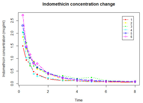
Figure 2. Indomethicin concentration (mcg/mL) of six individuals measured 11 times after injection.

From the plot, we can see that the initial decrease in the plasma concentration of the drug level is dramatic due to the movement of the drug from the body circulation system into the tissue, until an equilibrium is reached. We establish a non-linear mixed-model to describe the change. $y_{ij}={\beta }_{1}exp(-({\beta }_2+{\alpha }_i)t_j)+{ϵ}_{ij}$, where we assume ${\alpha }_i,i=1,\dots ,6$ to be random effects, which are independent and distributed as $N(0,{\tau }^2)$. ${ϵ}_{ij}$ are i.i.d random errors distributed as $N(0,{\sigma }^2)$, and ${\alpha }_i$ and ${ϵ}_{ij}$s are independent of each other. We use our method to estimate the parameter $\theta =({\beta }_1,{\beta }_2,\tau )$. The first-step estimate is ${\widehat{\theta }}_1=(2.910,1.539,0.533)$ and the second-step estimate is ${\widehat{\theta }}_2=(2.804,1.492,0.522)$. The results show that the first-step estimate is comparable to the second-step estimate.

Then, we estimate the parameter ${\sigma }^2$. In this model, $f(x_j,\beta ,{\alpha }_i)={\beta }_{1}exp(-({\beta }_2+{\alpha }_i)t_j)$. Then, we can obtain the first-step estimator ${\sigma }_1^2=0.021$ and second-step estimator ${\sigma }_2^2=0.021$. The two-step estimator returns the same estimate, so the first-step estimates are the ones to be used.

6.3. Orange Trees

We consider the data on the growth of orange trees over time given in Draper and Smith ([18] Exercise 24.N, p.559), described in [4]. The data are presented in Figure 3 and consist of seven measurements of the trunk circumferences (in millimeters) of five trees on seven occasions.

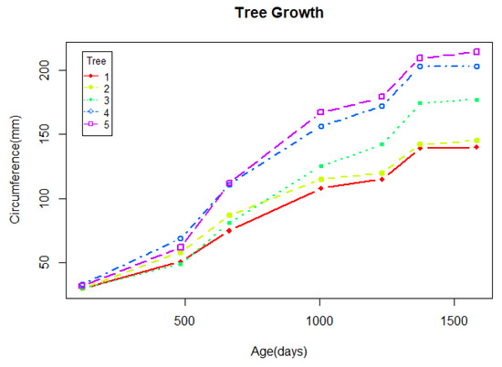
Figure 3. Trunk circumference (in millimeters) of five orange trees.

Each of the five trees was measured at 118, 484, 664, 1004, 1231, 1372, and 1582 days after December 31, 1968, when the study started. Let $y_{ij}$ be the trunk circumferences (in millimeters) for the $ith$ tree at $jth$ time. We consider a non-linear model as follows:

$$\begin{array}{c}\hfill y_{ij}=\frac{{\beta }_1}{1+exp\{-[t_j/365.25-({\beta }_2+{\alpha }_i)]\}}+{ϵ}_{ij},i=1,\dots ,5;j=1,\dots ,7,\end{array}$$

where $t_j$ represents the day corresponding to the $jth$ measurement; ${\alpha }_i,i=1,\dots ,5$ are independent random effects, identically distributed as $N(0,{\tau }^2)$; and ${ϵ}_{ij},i=1,\dots ,5;j=1,\dots ,7$ are the random errors, assumed to be independent and distributed as $N(0,{\sigma }^2)$. ${\alpha }_i$ and ${ϵ}_{ij}$ are independent of each other. We use our method to estimate the parameter $\theta =({\beta }_1,{\beta }_2,\tau )$. The first-step estimate is ${\widehat{\theta }}_1=(204.960,2.158,0.577)$, and the second-step estimate is ${\widehat{\theta }}_2=(204.960,2.159,0.591)$. If the iteration converges, we can obtain the estimate $\widehat{\theta }=(204.961,2.169,0.673)$. The results show that the two-step estimate is similar to the converged estimate. We use the second-step estimate for subsequent work. For ${\sigma }^2$, we can obtain the first-step estimator ${\sigma }_1^2=204.686(\sigma =14.306)$ and second-step estimator ${\sigma }_2^2=204.579(\sigma =14.303)$. It is shown that the two-step estimate is very close.

7. Concluding Remarks

In this paper, we propose a two-step method to estimate the parameters, and we study the asymptotic properties of the estimators. This method is very convenient to use because it depends only on $E(y_{ij})$ and we do not have to know the special distribution of $y_{ij}$. On the other hand, this method can only estimate the parameters related to $E(y_{ij})$. Thus, we need some other method to estimate other parameters. Here, we provide a method to estimate the variance ${\sigma }^2$ using the method of moments.

We found that the second-step estimate is sometimes not more efficient than the first-step estimate, or that it demonstrates little improvement. In such a case, we choose to use the first-step estimate, which is simpler and computationally more attractive.

In this paper, the numerical solution is also an important topic. Hence, we will attempt to improve our numerical solution method in future work; see [19,20,21].

References

- FDA US. Guidance for Industry: Population Pharmacokinetics; FDA: Rockville, MD, USA, 1999. [Google Scholar]
- Jiang, J.; Ge, Z. Mixed models: An overview. In Frontiers of Statistics in Honor of Professor Peter J. Bickel’s 65th Birthday; Fan, J., Koul, H., Eds.; Imperial College Press: London, UK, 2006; pp. 445–466. [Google Scholar]
- Gelman, A.; Carlin, J.; Stern, H.; Rubin, D. Bayesian Data Analysis, 2nd ed.; Chapman & Hall/CRC: Boca Raton, FL, USA, 2004. [Google Scholar]
- Lindstrom, M.; Bates, D. Nonlinear mixed effects models for repeated measures data. Biometrics 1990, 46, 673–687. [Google Scholar] [CrossRef] [PubMed]
- Pinheiro, J.; Bates, D. Approximations to the Log-likelihood function in Nonlinear Mixed Effects Models. J. Comput. Graph. Stat. 1995, 4, 12–35. [Google Scholar]
- Geweke, J. Bayesian Inference in Econmetric Models Using MonteCarlo Integration. Econometrica 1989, 57, 1317–1339. [Google Scholar] [CrossRef]
- Davidian, M.; Gallant, A.R. Smooth Nonparametric Maximum Likelihood Estimation for Population Pharmacokinetics, with Application to Quinidine. J. Pharmacokinet. Biopharm. 1992, 20, 529–556. [Google Scholar] [CrossRef] [PubMed]
- Jiang, J. Linear and Generalized Linear Mixed Models and Their Applications; Springer: New York, NY, USA, 2007. [Google Scholar]
- Jiang, J.; Nguyen, T. Linear and Generalized Linear Mixed Models and Their Applications, 2nd ed.; Springer: New York, NY, USA, 2021. [Google Scholar]
- Jiang, J.; Luan, Y.; Wang, Y.G. Iterative Estimating Equations: Linear Convergence and Asymptotic Properties. Ann. Stat. 2007, 35, 2233–2260. [Google Scholar] [CrossRef]
- Jiang, J. Asymptotic Analysis of Mixed Effects Models. Theory, Applications, and Open Problems; Chapman & Hall/CRC: Boca Raton, FL, USA, 2017. [Google Scholar]
- McCullagh, P. ; Nelder, J A. Generalised Linear Modelling; Chapman and Hall: New York, NY, USA, 1989. [Google Scholar]
- Jiang, J. A nonlinear Gauss–Seidel algorithm for inference about GLMM. Comput. Stat. 2000, 15, 229–241. [Google Scholar] [CrossRef]
- Jiang, J.; Zhang, W. Robust estimation in generalised linear mixed models. Biometrika 2001, 88, 753–765. [Google Scholar] [CrossRef]
- Stuart, H.C.; Reed, R.B. Longitudinal studies of child health and development, Harvard School of Public Health, Series II, No. 1, Description of project. Pediatrics 1929, 24, 875–885. [Google Scholar] [CrossRef]
- Demidenko, E. Mixed Models: Theory and Applications with R; John Wiley & Sons: New York, NY, USA, 2013. [Google Scholar]
- Pinheiro, J.; Bates, D. Mixed-Effects Models in S and S-PLUS; Statistics and Computing Series; Springer: New York, NY, USA, 2000. [Google Scholar]
- Draper, N.R.; Smith, H. Applied Regression Analysis, 3rd ed.; Wiley: New York, NY, USA, 1998. [Google Scholar]
- Qalandarov, A.A.; Khaldjigitov, A.A. Mathematical and numerical modeling of the coupled dynamic thermoelastic problems for isotropic bodies. TWMS J. Pure Appl. Math. 2020, 11, 119–126. [Google Scholar]
- Shokri, A.; Saadat, H. Trigonometrically fitted high-order predictor–corrector method with phase-lag of order infinity for the numerical solution of radial Schrödinger equation. J. Math. Chem. 2014, 52, 1870–1894. [Google Scholar] [CrossRef]
- Shokri, A.; Saadat, H. P-stability, TF and VSDPL technique in Obrechkoff methods for the numerical solution of the Schrodinger equation. Bull. Iran. Math. Soc. 2016, 42, 687–706. [Google Scholar]
Publisher’s Note: MDPI stays neutral with regard to jurisdictional claims in published maps and institutional affiliations. |
© 2022 by the authors. Licensee MDPI, Basel, Switzerland. This article is an open access article distributed under the terms and conditions of the Creative Commons Attribution (CC BY) license (https://creativecommons.org/licenses/by/4.0/).