Enhanced Marine Predators Algorithm for Solving Global Optimization and Feature Selection Problems

Abstract

Feature selection (FS) is applied to reduce data dimensions while retaining much information. Many optimization methods have been applied to enhance the efficiency of FS algorithms. These approaches reduce the processing time and improve the accuracy of the learning models. In this paper, a developed method called MPAO based on the marine predators algorithm (MPA) and the “narrowed exploration” strategy of the Aquila optimizer (AO) is proposed to handle FS, global optimization, and engineering problems. This modification enhances the exploration behavior of the MPA to update and explore the search space. Therefore, the narrowed exploration of the AO increases the searchability of the MPA, thereby improving its ability to obtain optimal or near-optimal results, which effectively helps the original MPA overcome the local optima issues in the problem domain. The performance of the proposed MPAO method is evaluated on solving FS and global optimization problems using some evaluation criteria, including the maximum value (Max), minimum value (Min), and standard deviation (Std) of the fitness function. Furthermore, the results are compared to some meta-heuristic methods over four engineering problems. Experimental results confirm the efficiency of the proposed MPAO method in solving FS, global optimization, and engineering problems.

1. Introduction

The curse of dimensionality is one of the most tackled topics in recent research. Many redundant unuseful noisy features might contaminate the feature space. Hence, the idea of feature selection (FS) has been prominent for many years. The literature classified FS methods into two main categories: filter and wrapper [1]. Filter methods take advantage of the statistical measures of the features. For example, it might eliminate or keep features based on their values. The filter method is fast but less sensitive to the used classifier [2]. Wrapper methods select subsets of the feature space and evaluate the classifier performance. However, they are computationally exhaustive and time consuming if the brute force search method is accommodated [3]. Here, the role of metaheuristic algorithms appears clearly. Metaheuristics algorithms can search the feature space for the best subset that achieves the highest classification accuracy [4].

Metaheuristic algorithms can be classified into four classes: (1) swarm intelligence algorithms, (2) human-based algorithms, (3) chemistry and physics algorithms, and (4) evolution algorithms. Swarm-based algorithms depend on studying the behavior of flocks and how they interact to reach food sources. Examples of such algorithms are the grasshopper optimization algorithm (GOA) [5], Harris hawk optimization [6], snake optimizer (SO) [7], and coot bird optimizer [8]. Human-based algorithms depend on simulating physical and nonphysical human behaviors. Such classes of algorithms include teaching learning-based optimization (TLBO) [9], social-based algorithm (SBA) [10], and imperialist competitive algorithm (ICA) [11]. Chemistry and physics algorithms are derived from chemical or physical laws such as ion motion algorithm [12], lightning search algorithm [13], and vortex search algorithm [14]. Evolution algorithms maintain the evolution process of biological creatures such as genetic algorithm (GA) [15], differential evolution (DE) [16], bacterial foraging optimization (BFO) [17], and memetic algorithm (MA) [18]. However, no free lunch theory [19] mentioned that if one optimization algorithm could solve some optimization problems, it might not be able to solve all problems. That provokes scientists to propose more algorithms or even enhance the established ones.

In 2020, the marine predator algorithm (MPA) was introduced by the authors of  [20]. Various foraging strategies of predators in biological interaction inspired the authors to develop MPA. The mathematical model of MPA mimics the behavior of marine predators’ foraging strategy in nature. MPA accommodates Lévy and Brownian statistical distributions. Lévy strategy searches the space with small steps associated with long jumps. Meanwhile, the Brownian strategy sweeps the search space in controlled and uniform steps. The virtue of the Lévy strategy is its deep and accurate search, while the Brownian strategy ensures visiting distant areas. This cooperation improved the searchability of MPA significantly. The statistical results showed that MPA outperformed the genetic algorithm (GA), cuckoo search (CS), gravitational search algorithm (GSA), particle swarm optimization (PSO), salp swarm algorithm (SSA), and covariance matrix adaptation evolution strategy (CMA-ES). The MPA also has indicated high execution in solving engineering issues. It shows a high convergence rate toward the global optimal and does not require training its parameters. However, applying the metaheuristic algorithm in solving various optimization problems is encouraged according to the “no free lunch” theory. Moreover, a new metaheuristic algorithm named Aquila optimizer (AO) was introduced in [21]. It is inspired by the hunting behavior of one of the most intelligent birds, Aquila, a dark brown bird belonging to the Accipitridae group. The AO was successfully applied to optimize the parameters of PID controllers [22] and multilevel inverters [23].

From the previous revision, we can summarize the novelty and contributions of the study in the following points:

• Improve the exploration phase of the MPA algorithm.
• Apply the “narrowed exploration” strategy of the AO in the MPA algorithm.
• Evaluate the proposed method using different optimization problems.

The rest of this paper is arranged as follows: Section 2 lists the related works. Section 2 describes the materials and methods. Section 4 presents the proposed method. Section 5 contains the experiments results and discussion, whereas the last section concludes the study.

2. Related Work

Although MPA has recently appeared as a metaheuristic algorithm, it suffers from early convergence. This drawback affects its accuracy in classification tasks. The authors in [24] improved this drawback by hybridizing MPA and simulated annealing (SM). SM has widened the MPA search space and improved its efficiency in FS tasks from high-dimensional datasets. Many metaheuristic algorithms successfully balance exploration and exploitation phases by embedding chaos theory. Chaos theory is an alternative method to generate random numbers in the algorithm. The authors in [25] introduced a chaotic MPA for feature selection. The practical results showed that the improved MPA had achieved the optimal number of features in many experiments. One of MPA’s drawbacks is its unidirectional search for prey. This drawback provoked the authors in [26] to embed opposition learning-based concepts [27] to allow the examination in all possible search directions. This improvement saves the MPA from stagnation in the local optima. The proposed method achieved the best convergence rate and selected the optimal feature set compared with other competitive algorithms. Again, the shortage of MPA search ability is addressed in [28]. The authors hybridize MPA with a sine cosine algorithm (SCA). Extensive experiments have been conducted to evaluate the performance of the proposed hybrid approach, and it showed its superiority in all accuracy measures.

The authors in [29] noticed that the prey movement of MPA depends on two simple strategies: levy flight and Brownian motion. The problem search space is too complex to be searched by those simple strategies. This note trapped the native MPA in local optima. They proposed a co-evolutionary cultural mechanism that divides the populations into subpopulations. Each subpopulation respects its search space and shares accumulated experiences with others. In addition, two operators are added to enhance the diversity of the populations and allow better experience exchange to support the exploitation of the native MPA. The proposed approach was tested in the FS task and proved its superiority over competitive algorithms. Moreover, it is used to optimize the parameters of the SVM algorithm.

The two most significant drawbacks of the MPA are the lack of population diversity and the bad convergence performance. In this regard, Gang et al. [30] tackled the weakness of MPA regarding population diversity. However new and successful in many applications, MPA solutions still need to be more accurate. They proposed an enhanced MPA by adding the neighborhood-based learning strategy and adaptive technique to control the population size. Their proposed approach was tested on state-of-the-art datasets for solving optimization problems and real-life applications. Compared with the original MPA, the enhanced version showed superior performance. Gang et al., again in 2021 [31], introduced a solution to the shape optimization problem of developable ball surfaces with hybrid MPA. The differential evolution algorithm combined MPA and a quasi-opposition strategy to help the original MPA jump out of local optima and enrich the population diversity. Their proposed approach effectively solved the shape optimization problem regarding robustness and precision.

As a new metaheuristic algorithm, MPA was applied in solving engineering problems in [32]. However, its convergence was treated by the following steps: (1) The logistic chaos function was used to ensure the quality of population diversity. (2) An adjustment transition strategy was added to maintain both exploration and exploitation. Moreover, the problem of falling into local optima was solved by updating the step information of predators by modifying the sigmoid function. Finally, after adding the golden sine factor, the proposed MPA achieved a better convergence rate, and its proposed solutions were diverse enough to solve engineering problems effectively.

MPA has been introduced to solve engineering and renewable energy problems such as predicting wind power in [33]. Mohamed et al. optimized the parameters of ANFIS (adaptive neuro-fuzzy inference system) using augmented MPA. In their augmented MPA, they added a mutation operator to the original MPA to overcome its sticking in local optima. The experiments revealed the competency of their modified MPA approach over many time-series forecasting algorithms.

Multilevel thresholding is an essential preprocessing step in image segmentation. Selecting the optimal threshold affects the accuracy of the segmented image. An improved MPA has been proposed in [34]; it proposed a strategy to steer the worst solutions toward the best ones and, at the same time, randomly in the search space to improve the convergence rate and prevent sticking in local optima. Another strategy is added to improve the exploration and exploitation capabilities. The experimental results showed the competency of the proposed MPA over other metaheuristic algorithms.

From the previous works, we can conclude that MPA has many drawbacks tackled in the previously mentioned proposed approaches, such as the problem of premature convergence, unidirectional search for prey, and sticking in local optima. The motivation of our research is to improve the weakness of the original MPA with the strength of another metaheuristic algorithm, Aquila optimizer (AO). Aquila optimizer was introduced in 2021 to solve continuous optimization problems. However, a binary version of AO is used for the wrapper approach FS from a medical dataset on COVID-19 [35]. Different shapes of transfer functions are applied to convert AO from its continuous nature into binary nature. The proposed approach proved its competencies in many directions, such as increasing accuracy, balancing exploration and exploitation, reducing the number of selected features, and fast convergence speed. Deep learning techniques inspired many researchers to use them as feature extraction methods and then apply AO for feature selection. In [36], the MobileNetV3 deep learning method extracted the features of some medical images. A binary thresholding version of AO selected the most non-trivial features to detect COVID-19 from X-ray images. The proposed method showed high performance and was suggested to cover many other areas of applications. However, the thresholding binary version of the AO optimizer is applied in intrusion detection in an IoT environment [37]. A deep learning technique based on CNN is used first for feature extraction, and then, the binary AO selects the most important features. This research confirmed that binary AO is competitive in many areas other than medical applications. The strength of the AO algorithm can treat the weakness of some metaheuristic algorithms. The hybrid combination of the Harris hawk algorithm with AO enhanced the searchability of the former. The proposed hybrid approach in [38] proved its competence in solving optimization problems. A hybrid algorithm that combined the exploration of AO and the exploitation of Harris hawk emerged in [39]. The robust search capability of AO is integrated with random opposition-based learning to enhance the Harris hawk optimization algorithm. An intensive study on its performance is introduced to test its exploration, exploitation, and sticking in local optima. The results show its superiority and its competence in solving industrial engineering problems.

3. Material and Methods

This section briefly describes the marine predators algorithm and Aquila optimizer.

3.1. Marine Predators Algorithm (MPA)

The MPA was presented in [20]. The biological ocean predators’ motions inspired it. The main steps of MPA are as follows:

• MPA initialization: As with all population-based algorithms, MPA has an initialization step where all populations are distributed uniformly in the search space as shown in Equation (1).

  $$X_0=u+\mathrm{rand}\left(l-u\right)$$

  (1)

  where u and l are the lower and upper bounds, respectively. $rand$ is a random vector in [0, 1]. The fittest solution $\overrightarrow{X^I}$ is selected to form a matrix called Elite shown in Equation (2). Elite matrix has a dimension $[n,d]$, where n is the search agents and n is the number of the problem dimension.

  $$\mathrm{Elite}={\left[\begin{array}{cccc}{X}_{1,1}^I& X_{1,2}^I& \cdots & X_{1,d}^I\\ X_{2,1}^I& X_{2,2}^I& \cdots & X_{2,d}^I\\ ⋮& ⋮& ⋮& ⋮\\ ⋮& ⋮& ⋮& ⋮\\ ⋮& ⋮& ⋮& ⋮\\ X_{n,1}^I& X_{n,2}^I& \cdots & X_{n,d}^I\end{array}\right]}_{n\times d}$$

  (2)
  Another matrix called Prey is constructed with the exact dimensions of Elite shown in Equation (3).

  $$\mathrm{Prey}={\left[\begin{array}{cccc}{X}_{1,1}& X_{1,2}& \cdots & X_{1,d}\\ X_{2,1}& X_{2,2}& \cdots & X_{2,d}\\ X_{3,1}& X_{3,2}& \cdots & X_{3,d}\\ ⋮& ⋮& ⋮& ⋮\\ ⋮& ⋮& ⋮& ⋮\\ X_{n,1}& X_{n,2}& \cdots & X_{n,d}\end{array}\right]}_{n\times d}$$

  (3)
  The process of MPA is split into three levels based on the difference in velocity ratio between a predator and prey.
• Predator moving faster than prey (exploration phase): When the prey is faster than the predator, the predator’s best strategy is to remain stationary. Exploration is more important in the first third of iterations. The prey position is updated by a $stesize$ calculated as shown in Equation (4).

  $${\overrightarrow{\mathrm{stepsize}}}_i={\overrightarrow{R}}_B\otimes \left({\overrightarrow{\mathrm{Elite}}}_i-{\overrightarrow{R}}_B{\overrightarrow{\otimes Prey}}_i\right),i=1,\dots ,n$$

  (4)

  where $R_B$ is a random numbers vector. The new prey position is updated as shown in Equation (5).

  $${\overrightarrow{\mathrm{Prey}}}_i={\overrightarrow{Prey}}_i+0.5·\overrightarrow{N}\otimes {\overrightarrow{\mathrm{stepsize}}}_i$$

  (5)

  where $\overrightarrow{N}$ is a random vector in [0, 1].
• Predator and prey are moving at the same rate (exploitation vs. exploration):
  When the predator and the prey move at the same speed, they are both on the prowl for prey. This section occurs during the intermediate stage of the optimization process when exploration attempts to be transiently converted to exploitation. It is critical for both exploration and exploitation. As a result, half of the population is used for exploration and the other half is used for exploitation. During this phase, the predator is in charge of exploration, while the prey is in charge of exploitation. The new positions for the first half of the populations (supporting exploitation) are updated as shown in Equation (6).

  $$\begin{array}{cc}\hfill {\overrightarrow{\mathrm{stepsize}}}_i& ={\overrightarrow{R}}_L\otimes \left({\overrightarrow{\mathrm{Elite}}}_i-{\overrightarrow{R}}_L\otimes {\overrightarrow{\mathrm{Prey}}}_i\right)i=1,\dots ,n/2\hfill \\ \hfill {\overrightarrow{\mathrm{Prey}}}_i& ={\overrightarrow{Prey}}_i+0.5·\overrightarrow{N}\otimes {\overrightarrow{\mathrm{stepsize}}}_i\hfill \end{array}$$

  (6)

  where ${\overrightarrow{R}}_L$ is a vector of random numbers based on Levy distribution. The new positions for the second half of the populations (supporting exploration) are updated as shown in Equation (7)

  $$\begin{array}{cc}\hfill {\overrightarrow{\mathrm{stepsize}}}_i& ={\overrightarrow{R}}_B\otimes \left({\overrightarrow{R}}_B\otimes {\overrightarrow{\mathrm{Elite}}}_i-{\overrightarrow{\mathrm{Prey}}}_i\right)i=n/2,\dots ,n\hfill \\ \hfill {\overrightarrow{\mathrm{Prey}}}_i& ={\overrightarrow{\mathrm{Elite}}}_i+0.5.A\otimes {\overrightarrow{\mathrm{stepsize}}}_i\hfill \end{array}$$

  (7)

  where A is a control parameter calculated as shown in Equation (8).

  $$\mathrm{A}={\left(1-\frac{\mathrm{Iter}}{MaxIter}\right)}^{\left(2\frac{\mathrm{Iter}}{\mathrm{MaxIter}}\right)}$$

  (8)
• Prey moving faster than predator (exploitation):
  This scenario occurs during the final stage of the optimization process and is typically associated with a high capacity for exploitation. The prey positions are updated as shown in Equation (9).

  $$\begin{array}{cc}\hfill {\overrightarrow{\mathrm{stepsize}}}_i& ={\overrightarrow{R}}_L\otimes \left({\overrightarrow{R}}_L\otimes {\overrightarrow{\mathrm{Elite}}}_i-{\overrightarrow{\mathrm{Prey}}}_i\right),i=1,\dots ,n\hfill \\ \hfill {\overrightarrow{\mathrm{Prey}}}_i& ={\overrightarrow{\mathrm{Elite}}}_i+0.5.\mathrm{A}\otimes {\overrightarrow{\mathrm{stepsize}}}_i\hfill \end{array}$$

  (9)
  To maintain the search, the Fish Aggregating Devices (FADs) is proposed. The mathematical model of FADs is defined in Equation (10). Algorithm 1 shows the pseudo code of the MPA.

  $$\overline{\mathrm{preyl}{}_l}=\left\{\begin{array}{c}\overline{\mathrm{prey}{}_i}+CF\left[X_{min}+\overrightarrow{R}\otimes \left({\overline{X}}_{max}-{\overline{X}}_{min}\right)\right]\otimes \overrightarrow{U}\hfill \\ \mathrm{if}r\le \mathrm{FADs}\hfill \\ \overrightarrow{\mathrm{prey}{}_l}+[\mathrm{FADs}(1-r)+r]\left(\overline{\mathrm{prey}1}-\overline{\mathrm{prey}{}_{r2}}\right)\hfill \\ \mathrm{if}r>\mathrm{FADs}\hfill \end{array}\right.$$

  (10)

Algorithm 1 MPA pseudo code

1: initialize populations. t = 1.   2: while$(t<=Tmax)$do   3:     Calculate the fitness and form the Elite matrix.   4:     if $t<Tmax/3$ then   5:         Update the prey position based on Equation (5).   6:     else if $Tmax/3<t<2\ast Tmax/3$ then   7:         For the first half of the populations, update prey position based on Equation (6).   8:         For the other half, use Equation (7) to update the position.   9:     else if $t>2\ast Tmax/3$ then 10:         Update prey position using Equation (9). 11:     end if 12:     Apply memory saving and Elite update 13:     Apply FAD effect using Equation (10) 14:     Apply memory saving and Elite update 15:     $t=t+1$ 16: end while 17: return the best position.

3.2. Aquila Optimizer (AO)

AO [21] was introduced in 2021 as an optimization algorithm. The algorithm mimics Aquila hunting behavior and has four main stages: initialization, exploration, exploitation, and finally, reaching the optimal solution. The initialization stage starts by initializing population X with N agents as shown in Equation (11).

$$X_{ij}=r_1\times (U{B}_j-L{B}_j)+L{B}_j,i=1,2,.....,Nj=1,2,...,Dim$$

(11)

where $U{B}_j$ and $L{B}_j$ are the upper and lower bounds of the search space, the number of problem dimensions is $Dim$, and $r_1\in [0,1]$ is the random value.

The next phase of the AO approach is to either explore or exploit until the best solution is identified. According to [21], there are two methods for both exploration and exploitation. The first technique uses the best agent ($X_b$) and the average of all agents ($X_M$) to carry out the exploration. The mathematical formulation of this method is as follows:

$$X_i(t+1)=X_b\left(t\right)\times \left(\frac{1-t}{T}\right)+(X_M\left(t\right)-X_b\left(t\right)\ast rand),$$

(12)

$$X_M\left(t\right)=\frac{1}{N}\sum _{i=1}^{N}X\left(t\right),\forall j=1,2,...,Dim$$

(13)

T declares the max iteration’s number.

The second method, expressed as follows, uses $X_b$ and the Levy flight $Levy\left(D\right)$ distribution to improve the solutions’ ability for exploration.

$$X_i(t+1)=Levy\left(D\right)\times X_b\left(t\right)+X_R\left(t\right)+(y-x)\ast rand,$$

(14)

$$Levy\left(D\right)=s\times \frac{u\times \sigma }{{\left|\upsilon \right|}^{\frac{1}{\beta }}},\sigma =\left(\frac{sine\left(\frac{\pi \beta }{2}\right)\times \Gamma (1+\beta )}{\beta \times 2^{\left(\frac{\beta -1}{2}\right)}\times \Gamma \left(\frac{1+\beta }{2}\right)}\right)$$

(15)

where u and $\upsilon$ are random numbers; while $s=0.01$ and $beta=1.5$ are constants. $X_R$ is a randomly chosen agent in Equation (14). In addition, y and x are used to mimic the spiral shape, and they are written as:

$$y=r\times cos\left(\theta \right),x=sin\left(\theta \right)\times r$$

(16)

$$r=r_1+U\times D_1,\theta =-\omega \times D_1+{\theta }_1,\theta 1=\frac{3\times \pi }{2}$$

(17)

where $\omega =0.0050$ and $U=0.005650$ are random values, and $r_1\in [0,20]$ is a random number.

The first technique is used in [21] in the exploitation phase based on $Xb$ and $XM$ and it is computed as:

$$X_i(t+1)=(X_b\left(t\right)-X_M\left(t\right))\times \alpha -rand+((UB-LB)\times rand+LB)\times \delta ,$$

(18)

The parameters for exploitation adjustment are given by $\alpha$ and $\delta$. A random value is the value rand [0, 1].

The solution is updated using $Levy$, $X_b$, and the quality function $QF$ in the second exploitation phase. That is defined as follows:

$$X_i(t+1)=QF\times X_b\left(t\right)-(G_1\times X\left(t\right)\times rand)-G_2\times Levy\left(D\right)+rand\times G_1,$$

(19)

$$QF\left(t\right)=t^{\frac{2\times rand\left(\right)-1}{{(1-T)}^2}}$$

(20)

In addition, $G_1$ refers to several motions used to track the optimal solution as in Equation (21).

$$G_1=2\times rand\left(\right)-1,G_2=2\times (1-\frac{t}{T})$$

(21)

A random value is denoted by the symbol $rand$. $G_2$, on the other hand, denotes decreasing values from 2 to 0, and it is calculated as:

$$G_2=2\times (1-\frac{t}{T})$$

(22)

4. Proposed Method

This section describes the proposed MPAO method. This method aims to improve the optimization technique of the original MPA using the strategy of the narrowed exploration of the AO. This modification enhances the exploration behavior of the MPA to update the search space and explore more regions in the search domain. Therefore, the narrowed exploration of the AO increases the searchability of the MPA, thereby improving its ability to obtain optimal or near-optimal results. This phase effectively helps the original MPA overcome the local optima issues in the problem domain. The narrowed exploration of the AO is applied based on a random variable $rx$, where $rx\in [0,1]$. If $rx$ is greater than 0.25, the narrowed exploration (Equation (14)) is applied, else the operators of MPA (Equation (7)) are used.

The optimization process of MPAO starts by determining the values of all parameters and creates the initial population for the search space. Then, the fitness function ($f\left(x\right)$) checks the solutions’ quality using Equation (23); if the current solution is better than the old one, the MPAO saves it as the best solution.

$$f\left(x\right)=\gamma C_x+(1-\gamma )\left(\frac{s}{S}\right)$$

(23)

where $\gamma C_x$ denotes the error of the classification phase (in this study, the K-NN is used as a classifier). The second part of the equation defines the selected feature’s ratio (s). S denotes the number of full features. $\gamma$ is a random value in $[0,1]$.

After that, the optimization begins by discovering the search space and evaluating the solutions using the fitness function to determine the initial optimal values.

In the second–third part of the optimization process, the MPAO decides to update the solutions using the MPA or AO based on a random value. This step helps with improving the exploration phase and adds more diversity to the search space. Finally, all obtained values by the fitness function are checked; then, the best one is selected and saved. The above steps can be summarized as follows:

• Declare the experiment variables and their values.
• Generate the X population randomly with a specific size and dimension.
• Start the main loop of the MPAO.
• Apply the fitness function for all solutions.
• Return the best value.

The above steps are iterated until reaching the stop condition. The structure of the MPAO is presented in Figure 1.

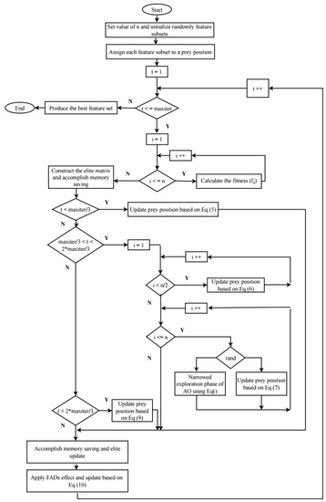
Figure 1. Proposed MPAO architecture.

5. Experiments and Discussion

This section evaluates the proposed MPAO using three experiments: solving global optimization problems, selecting the essential features, and solving real engineering problems. The proposed method is compared with nine optimization methods: PSO [40], GA [41], AO [21], MFO [42], MPA [20], SSA [43], GOA [5], slime mold algorithm (SMA) [44], and whale optimization algorithm (WOA) [45]. Table 1 lists the parameter settings for all of them.

Table 1. Parameter settings.

Algorithm	Parameters Values
GA	$\gamma$ = 0.2, pm = 0.3, pc = 0.8, $\beta$ = 8, mu = 0.02
PSO	w = 1, C1 and C2 = 1, wDamp = 0.990
WOA	b = 1.0, a = [0, 2], l = [−1, 1]
SSA	$C_3$∈ [0, 1], $C_2$ ∈ [0, 1]
MPA	P = 0.50, $\beta$ = 1.50, FADs = 0.20
AO	$\delta$ = 0.1, $\alpha$ = 0.1
SMA	z = 0.030
GOA	$c_{max}=1.00$, $c_{min}=0.000040$
MFO	a = $\in [-2-1]$, b = 1
MPAO	P = 0.50, FADs = 0.20, $\beta$ = 1.50, $\alpha$ = 0.1, $\delta$ = 0.1

In the experiments, there are some performance measures used to evaluate the proposed method, namely: the average, minimum (Min), standard deviation (Std), and maximum (Max) values of the fitness function as in Equations (24)–(26), respectively. In addition, the classification accuracy is as in Equation (27).

$$Max=\underset{1\le i\le N}{max}{f}_b^i$$

(24)

$$Min=\underset{1\le i\le N}{min}{f}_b^i$$

(25)

$$Std=\sqrt{\frac{1}{N}\sum _{i=1}^N{|f_i-\mu |}^2}$$

(26)

where f and $\mu$ denote the value and mean of the objective function, respectively. N denotes the size of the sample.

$$Acc=\frac{TP+TN}{TP+FN+FP+TN}$$

(27)

where $TN$ and $TP$ denote true negative and positive results, respectively. $FN$ and $FP$ denote false negative and positive results.

5.1. Experiment 1: Global Optimization

This experiment discusses the experimental results using the CEC2019 benchmark [46] by comparing the MPAO to some state-of-the-art advanced competitors, including PSO, GA, AO, MFO, SMA, MPA, SSA, GOA, and WOA. Table 2, Table 3, Table 4 and Table 5 report the results of average fitness, Std, Max, and Min over ten test functions of the CEC 2019 benchmark. In all tables, the boldface refers to the best value.

Table 2. Average of the fitness function.

Fitness	MPAO	PSO	GA	AO	MFO	SMA	MPA	SSA	GOA	WOA
F1	$9.8\times {10}^7$	$5.4\times {10}^{12}$	$6.4\times {10}^{10}$	$\mathbf{7}.\mathbf{2}\times {\mathbf{10}}^{\mathbf{4}}$	$3.9\times {10}^{10}$	$1.3\times {10}^8$	$2.0\times {10}^8$	$3.2\times {10}^{10}$	$1.0\times {10}^{12}$	$2.4\times {10}^{11}$
F2	17.3429	17572.6	24.0539	17.4253	17.3762	17.3493	17.3438	17.7506	4835.64	17.5476
F3	12.7024	12.7024	12.7024	12.7025	12.7024	12.7029	12.7024	12.7029	12.7043	12.7024
F4	37.328	2655.65	103.248	3888.51	111.354	43.323	66.652	86.691	6347.84	2244.70
F5	1.1493	2.4856	1.1707	2.3692	1.3942	1.5244	1.2688	1.1931	3.1950	2.3165
F6	5.3995	11.3959	6.9637	11.6460	6.9047	10.0283	5.1793	7.9303	10.5355	10.3370
F7	128.129	369.736	230.85	678.72	455.91	413.32	171.96	414.07	890.94	812.84
F8	4.6566	6.0968	5.4827	6.2123	5.3837	5.7392	4.7533	5.7522	6.9650	6.1076
F9	3.3087	60.8198	3.3120	262.603	3.7325	3.1231	3.3268	3.8415	906.81	177.21
F10	20.012	20.530	20.174	20.626	20.143	20.499	18.800	20.096	20.522	20.499

Table 3. Average of the standard deviation of the fitness function.

Fitness	MPAO	PSO	GA	AO	MFO	SMA	MPA	SSA	GOA	WOA
F1	$2.5\times {10}^7$	$5.5\times {10}^{12}$	$5.9\times {10}^{10}$	$\mathbf{1}.\mathbf{8}\times {\mathbf{10}}^{\mathbf{8}}$	$5.0\times {10}^{10}$	$5.0\times {10}^8$	$2.1\times {10}^8$	$4.1\times {10}^{10}$	$1.1\times {10}^{12}$	$2.2\times {10}^{11}$
F2	0.0000	4545.32	20.7697	0.0456	0.0253	0.0029	0.0036	1.2910	1814.2625	0.1412
F3	$\mathbf{4}.\mathbf{3}\times {\mathbf{10}}^{\mathbf{12}}$	$4.2\times {10}^7$	$5.3\times {10}^7$	$4.9\times {10}^5$	$3.8\times {10}^5$	$7.0\times {10}^4$	$3.4\times {10}^9$	$1.0\times {10}^3$	$1.1\times {10}^3$	$1.5\times {10}^5$
F4	13.812	1755.848	66.809	1123.78	56.374	14.788	13.079	38.264	3601.57	1079.32
F5	0.0681	0.6314	0.0927	0.3748	0.2057	0.1892	0.0825	0.0872	0.4821	0.4346
F6	0.7966	0.9099	1.1223	0.7444	1.2010	1.3071	1.1628	1.3740	1.0611	1.0808
F7	121.125	304.895	186.871	209.602	295.891	247.995	131.941	266.407	219.64	145.75
F8	0.5416	1.0492	0.6554	0.4344	0.9944	0.4929	0.4285	0.5523	0.2950	0.7153
F9	0.7371	65.122	0.5731	173.339	0.6670	0.4946	0.3884	0.9028	540.447	123.834
F10	0.0138	0.1439	0.0570	0.1041	0.1351	0.1073	3.4481	0.1349	0.1660	0.1516

Table 4. Minimum values of the fitness function.

Fitness	MPAO	PSO	GA	AO	MFO	SMA	MPA	SSA	GOA	WOA
F1	$5.9\times {10}^7$	$3.5\times {10}^{11}$	$4.2\times {10}^9$	$5.2\times {10}^4$	$2.4\times {10}^9$	$\mathbf{5}.\mathbf{1}\times {\mathbf{10}}^{\mathbf{4}}$	$2.3\times {10}^7$	$5.9\times {10}^9$	$3.1\times {10}^{11}$	$2.3\times {10}^{10}$
F2	17.343	10314.099	17.343	17.360	17.345	17.345	17.343	17.344	2150.473	17.354
F3	12.702	12.702	12.703	12.703	12.703	12.703	12.703	12.703	12.703	12.703
F4	16.221	501.030	17.183	1846.99	57.768	24.489	44.514	26.620	1674.01	803.47
F5	1.0523	1.6612	1.0569	1.7537	1.1214	1.2652	1.1761	1.0640	2.4857	1.6620
F6	3.6330	9.6109	3.8354	9.9305	4.4174	7.0427	3.3423	5.8103	8.8478	8.6721
F7	−78.041	−121.72	−57.655	306.11	−59.043	158.51	−50.040	−76.690	460.78	634.57
F8	3.7175	3.3291	4.3536	5.6299	2.5838	5.0209	4.1234	4.6728	6.5461	4.2988
F9	2.5474	3.3357	2.5675	62.940	2.7396	2.5927	2.8640	2.9346	284.771	5.946
F10	19.996	20.159	20.048	20.402	20.002	20.310	6.7125	19.978	20.163	20.260

Table 5. Maximum values of the fitness function.

Fitness	MPAO	PSO	GA	AO	MFO	SMA	MPA	SSA	GOA	WOA
F1	$1.4\times {10}^8$	$1.9\times {10}^{13}$	$1.9\times {10}^{11}$	$\mathbf{1}.\mathbf{2}\times {\mathbf{10}}^{\mathbf{5}}$	$2.1\times {10}^{11}$	$2.1\times {10}^9$	$7.3\times {10}^8$	$1.7\times {10}^{11}$	$5.3\times {10}^{12}$	$9.3\times {10}^{11}$
F2	17.343	25684.6	101.158	17.530	17.451	17.355	17.357	22.572	8464.21	17.776
F3	12.702	12.702	12.702	12.703	12.703	12.705	12.702	12.706	12.706	12.702
F4	58.729	7440.74	308.29	5653.4	264.87	74.431	91.710	168.851	16776.6	4751.8
F5	1.2820	4.4236	1.3790	3.1667	2.0734	1.9849	1.4228	1.3566	4.0174	3.2375
F6	6.5206	13.6429	8.5646	12.6687	8.4957	11.8549	7.6363	10.4369	12.5073	12.3857
F7	307.33	866.88	596.19	1062.45	1098.39	908.58	456.60	893.19	1371.84	1067.62
F8	5.5873	7.1162	6.8344	6.9835	6.5186	6.7966	5.6520	6.5570	7.5365	7.4462
F9	5.1445	197.777	4.5874	618.10	5.3925	4.3462	4.2065	6.3094	2167.1	462.86
F10	20.046	20.703	20.257	20.835	20.489	20.696	20.039	20.403	20.746	20.784

Concerning the average of function fitness which is computed for all the counterparts, it is clear from Table 2 that the proposed MPAO is superior in six out of 10 functions (F2–F5 and F7–F8), followed by the MPA, which is better in three functions (F3, F6, and F10). On the other hand, the PSO, GA, MFO, and WOA show the best values in only one out of 10 functions. The SSA and GOA failed to realize the best files over all the functions.

The Std values show the stability in the results obtained by the competitors over the testing functions, which are reported in Table 3. The proposed MPAO shows lower Std values in five out of ten functions (F2, F3, F5, F7, and F10), which reflects the stability of the algorithm in most testing functions. The MFO comes in the second rank, stable over only two functions (F4 and F9), whereas the other competitors did not show stability over all the algorithms.

Table 4 reports the Max values computed from each counterpart’s fitness value of the testing functions. The MPAO reports the Max value in the majority of functions (F2–F8), followed by the MPA that shows the maximal over two functions only (F9–F10). The rest of the competing algorithms cannot provide any maximum value in all the testing functions.

Table 5 presents the Min values of fitness computed for the counterparts over the testing functions. The MPAO shows lower values in five functions (F2–F5 and F9), followed by PSO and MPA, each of which shows lower values in only two functions. Each MFO and SMA obtains the lower values in only one function, namely F8 and F1 means no substantial changes over the experiments. Table 5 demonstrates the Std values, where the MPAO realizes the lower value over seven out of 15 datasets. The PSO is only in three, the MFO in two, and the GA and MPA in one. In contrast, the other counterparts did not realize the best results over any datasets.

5.2. Experiment 2: Feature Selection

This experiment evaluates a set of UCI datasets by the proposed method. These benchmark datasets are collected from distinct fields such as biology, electromagnetic, games, physics, politics, and chemistry. Furthermore, each benchmark shows a different number of instances, features, and categories. The description of each benchmark is provided in Table 6.

Table 6. Description of the UCI datasets.

	Instances	Features	Classes
ionosphere	351	34	2
breastcancer	699	9	2
glass	214	9	7
sonar	208	60	2
lymphography	148	18	2
waveform	5000	40	3
clean1data	476	166	2
SPECT	267	22	2
ecoli	336	7	8
CongressEW	435	16	2
Exactly2	1000	13	2
M-of-n	1000	13	2
Vote	300	16	2
krvskp	3196	36	2
heart	270	13	2

Concerning this subsection, we demonstrate and discuss the experimental results of the comparisons conducted to solve the feature selection issue. These comparisons involved the proposed MPAO, PSO [40], GA [41], AO [21], MFO [42], SMA [44], MPA [20], SSA [43], GOA [5], and WOA [45] with the previously described evaluation metrics. Table 7 demonstrates the experimental results of the average of the fitness function, which were calculated for all compared counterparts over the 15 datasets. From the table, it is clear that the proposed MPAO was superior in 13 out of 15 datasets, whereas the PSO demonstrated the best values in three cases, which is followed by the MPA and SSA, each of which was better in one dataset. These results indicated that the MPAO was accurate and superior in the average measure of the fitness value. In all tables, the boldface refers to the best value. Keeping on with the fitness values, we can analyze the fitness functions’ maximum (Max) and minimum (Min) values. This investigation allows us to determine when the algorithms realize the worst and best value.

Table 7. Results of the average of the fitness value.

	MPAO	PSO	GA	AO	MFO	SMA	MPA	SSA	GOA	WOA
ionosphere	0.1233	0.1452	0.1918	0.2465	0.2657	0.4117	0.1237	0.1664	0.2025	0.1569
breastcancer	0.1088	0.1309	0.1587	0.2234	0.2536	0.4182	0.1164	0.1620	0.2037	0.1800
glass	0.1517	0.1662	0.1664	0.1926	0.2085	0.2801	0.1666	0.9691	1.0155	0.9730
sonar	0.0433	0.0790	0.1203	0.2823	0.2829	0.4832	0.0568	0.2379	0.2759	0.2759
lymphography	0.2656	0.3040	0.3371	0.4227	0.4687	0.6394	0.3051	0.3495	0.3888	0.3888
waveform	0.6363	0.6269	0.6426	0.6660	0.6685	0.9424	0.6345	0.6590	0.6786	0.6701
clean1data	0.1585	0.1916	0.2070	0.2804	0.2505	0.4712	0.1723	0.2296	0.2630	0.2616
SPECT	0.3095	0.3361	0.3500	0.3978	0.4210	0.5200	0.3372	0.3152	0.3377	0.3587
ecoli	0.2452	0.2488	0.2483	0.2499	0.3393	0.4143	0.2476	1.6245	1.5579	1.6245
CongressEW	0.0913	0.1185	0.1417	0.2052	0.2785	0.3823	0.1108	0.2064	0.1981	0.1820
Exactly2	0.4766	0.4849	0.4896	0.4986	0.5410	0.5818	0.4796	0.4865	0.4965	0.4953
M-of-n	0.0000	0.0000	0.0129	0.2142	0.4827	0.5707	0.0000	0.0000	0.1193	0.0298
Vote	0.1395	0.1642	0.1745	0.2511	0.2961	0.3957	0.1511	0.1802	0.1858	0.1755
krvskp	0.1274	0.1134	0.1476	0.3156	0.1708	0.5600	0.1236	0.1578	0.2224	0.1879
heart	0.3317	0.3538	0.3644	0.4737	0.4441	0.5671	0.3496	0.3665	0.4426	0.3850

Table 8 demonstrates the Min values of fitness obtained by the counterparts over all the datasets. The MPAO, PSO, and MPA showed lower values in most datasets, 13, 11, and 8 of the 15 datasets, respectively, as these algorithms could reach the optimal values.

Table 8. Results of the minimum value of the fitness value.

	MPAO	PSO	GA	AO	MFO	SMA	MPA	SSA	GOA	WOA
ionosphere	0.0000	0.0000	0.1066	0.1066	0.2132	0.2132	0.0000	0.1508	0.1846	0.1066
breastcancer	0.0000	0.0000	0.0000	0.0000	0.1508	0.1508	0.0000	0.1508	0.1846	0.1508
glass	0.0911	0.0911	0.0911	0.0911	0.1229	0.1602	0.1166	0.7891	1.0000	0.8009
sonar	0.0000	0.0000	0.0000	0.1961	0.1387	0.1961	0.0000	0.1961	0.2402	0.2402
Lymphography	0.1644	0.1644	0.1644	0.2325	0.3288	0.3288	0.2325	0.2847	0.3288	0.3288
waveform	0.5940	0.5973	0.6073	0.6177	0.6151	0.6876	0.5980	0.6456	0.6603	0.6621
clean1data	0.1296	0.1296	0.0917	0.2050	0.1833	0.2750	0.0917	0.2050	0.2425	0.2050
SPECT	0.2443	0.2443	0.2443	0.2732	0.2993	0.3455	0.2732	0.2993	0.3232	0.3232
ecoli	0.2014	0.2014	0.2014	0.2014	0.2038	0.2518	0.2014	1.5000	1.3002	1.5000
CongressEW	0.0000	0.0000	0.0000	0.0958	0.1916	0.1355	0.0000	0.0958	0.1659	0.1659
Exactly2	0.4336	0.4427	0.4382	0.4382	0.4775	0.4733	0.4382	0.4517	0.4817	0.4940
M-of-n	0.0000	0.0000	0.0000	0.0000	0.2966	0.0000	0.0000	0.0000	0.0000	0.0000
Vote	0.0000	0.1155	0.1155	0.1155	0.2000	0.2000	0.0000	0.1633	0.1633	0.1633
krvskp	0.1001	0.0791	0.1001	0.1119	0.1001	0.2347	0.0867	0.1415	0.2093	0.1697
heart	0.2443	0.2443	0.2732	0.3232	0.3232	0.4232	0.2732	0.3665	0.3863	0.3455

On the other side, Table 9 demonstrates the Max values of the fitness function, which were obtained during the conducted experiments using the counterparts across the 15 datasets of the UCI. The MPAO obtained the Max values over most cases (10 out of 15 datasets), followed by the SSA (only in six cases), MPA (in five cases) and WOA (in four cases). The other algorithms, including GA, AO, MFO, and SMA, could not provide any maximal values over all the experiments.

Table 9. Results of the maximum value of the fitness value.

	MPAO	PSO	GA	AO	MFO	SMA	MPA	SSA	GOA	WOA
ionosphere	0.2132	0.2384	0.2611	0.3693	0.3371	0.8394	0.2132	0.2132	0.2384	0.2132
breastcancer	0.1846	0.2384	0.2384	0.3844	0.3371	0.6124	0.1846	0.1846	0.2132	0.2384
glass	0.2146	0.2442	0.2442	0.2649	0.2788	0.4274	0.2881	1.0903	1.0370	1.0903
sonar	0.1387	0.1961	0.2774	0.4160	0.3922	0.7071	0.1961	0.2774	0.3101	0.3101
lymphography	0.4350	0.4932	0.5452	0.6975	0.6576	0.8383	0.4350	0.4350	0.4350	0.4350
waveform	0.6711	0.6591	0.6741	0.7642	0.7244	1.1398	0.6627	0.6765	0.6997	0.6794
clean1data	0.2050	0.2593	0.2899	0.3780	0.3430	0.5941	0.2750	0.2593	0.3040	0.2899
SPECT	0.3455	0.5037	0.5183	0.5183	0.6229	0.8725	0.4887	0.3232	0.3665	0.3863
ecoli	0.3094	0.3225	0.3225	0.3225	0.5876	0.7949	0.3225	1.6868	1.6868	1.6868
CongressEW	0.1916	0.2142	0.2142	0.3453	0.4175	0.7663	0.1916	0.3318	0.2142	0.2142
Exactly2	0.5177	0.5177	0.5477	0.6000	0.6033	0.7183	0.5215	0.5138	0.5138	0.4980
M-of-n	0.0000	0.0000	0.2449	0.5899	0.6132	0.8319	0.0000	0.0000	0.3578	0.0894
Vote	0.2309	0.2309	0.2582	0.4000	0.5538	0.6110	0.2309	0.2309	0.2309	0.2000
krvskp	0.1621	0.1415	0.2152	0.5318	0.3744	0.7242	0.1459	0.1659	0.2399	0.2001
heart	0.3665	0.4232	0.4405	0.5859	0.5730	0.7727	0.4232	0.3665	0.5183	0.4232

The results’ stability was calculated for each algorithm and analyzed based on the standard deviation (Std) measure. The Std was computed for the independent experiments over each benchmark by setting the fitness as the input value. In this regard, the lower Std refers to better stability for the results, which means no substantial changes over the experiments. Table 10 demonstrates the Std values, where the MPAO realized the lower value over seven out of 15 datasets. The PSO showed the best values in three datasets, the MFO in two, and the GA and MPA in only one. The other counterparts did not realize the best results over any datasets.

Table 10. Results of the standard deviation of the fitness value.

	MPAO	PSO	GA	AO	MFO	SMA	MPA	SSA	GOA	WOA
ionosphere	0.0623	0.0635	0.0455	0.0765	0.0436	0.1248	0.0578	0.0523	0.0661	0.0481
breastcancer	0.0602	0.0786	0.0688	0.0862	0.0414	0.1206	0.0647	0.0470	0.0562	0.0497
glass	0.0264	0.0391	0.0366	0.0446	0.0373	0.0792	0.0389	0.0326	0.0462	0.0253
sonar	0.0643	0.0768	0.0883	0.0649	0.0777	0.1514	0.0775	0.0839	0.0678	0.0858
lymphography	0.0910	0.0927	0.0931	0.1426	0.0901	0.1311	0.0747	0.0758	0.1163	0.0535
waveform	0.0195	0.0181	0.0195	0.0385	0.0296	0.1368	0.0191	0.0189	0.0555	0.0190
clean1data	0.0239	0.0331	0.0478	0.0446	0.0500	0.0755	0.0474	0.0455	0.0544	0.0417
SPECT	0.0346	0.0638	0.0688	0.0677	0.0738	0.1178	0.0509	0.0519	0.0651	0.0482
ecoli	0.0283	0.0321	0.0294	0.0297	0.1097	0.1517	0.0305	0.0379	0.1036	0.0243
CongressEW	0.0599	0.0619	0.0461	0.0792	0.0608	0.1638	0.0622	0.0691	0.1088	0.0463
Exactly2	0.0203	0.0206	0.0271	0.0376	0.0318	0.0713	0.0221	0.0412	0.0407	0.0263
M-of-n	0.0000	0.0000	0.0547	0.2399	0.0804	0.1568	0.0000	0.1100	0.1269	0.1248
Vote	0.0584	0.0332	0.0428	0.0777	0.1006	0.1164	0.0474	0.0675	0.0873	0.0443
krvskp	0.0138	0.0179	0.0305	0.1170	0.0693	0.1245	0.0157	0.0268	0.1164	0.0278
heart	0.0326	0.0460	0.0484	0.0700	0.0624	0.0863	0.0392	0.0390	0.0794	0.0452

The feature numbers resulting across all 15 datasets are reported in Table 11. The recorded results in that table are evidence of the efficacy and superiority of the MPAO algorithm. It obtained the best results in seven out of 15 datasets, showing the minor selected feature number that realizes high performance. It was followed by the SMA and the WOA, which achieved the least features in only three and two datasets, respectively, whereas the remaining algorithms were out of the competition.

Table 11. Ratio of the selected feature for all datasets.

	MPAO	PSO	GA	AO	MFO	SMA	MPA	SSA	GOA	WOA
ionosphere	0.2167	0.3963	0.4551	0.4078	0.4580	0.3775	0.2459	0.3162	0.4510	0.3627
breastcancer	0.2042	0.4350	0.4474	0.3971	0.4580	0.3072	0.2565	0.4706	0.5392	0.4216
glass	0.4667	0.5263	0.5906	0.5767	0.6085	0.4848	0.5185	0.7407	0.5556	0.7407
sonar	0.3167	0.5035	0.4930	0.5258	0.5254	0.4472	0.3913	0.5444	0.5167	0.4000
lymphography	0.3920	0.5088	0.5439	0.5152	0.5132	0.4545	0.4815	0.4630	0.4815	0.5000
waveform	0.6138	0.6917	0.7093	0.7987	0.6757	0.3129	0.7352	0.6667	0.5873	0.8730
clean1data	0.2523	0.4896	0.5060	0.3951	0.5066	0.2584	0.3330	0.4578	0.4759	0.5040
SPECT	0.3427	0.5024	0.5000	0.5475	0.5541	0.4788	0.4255	0.3788	0.4242	0.2273
ecoli	0.6484	0.7895	0.7744	0.8027	0.5238	0.5238	0.7714	0.6667	0.8095	0.7619
CongressEW	0.3462	0.4868	0.4803	0.4205	0.4821	0.3490	0.3850	0.5417	0.4792	0.2083
Exactly2	0.3522	0.5830	0.5020	0.1888	0.5568	0.3897	0.3877	0.3590	0.5641	0.5641
M-of-n	0.5240	0.5668	0.5547	0.6818	0.5531	0.4567	0.5354	0.5897	0.5128	0.5897
Vote	0.3438	0.4605	0.4803	0.5795	0.4881	0.4808	0.3625	0.5156	0.5417	0.5000
krvskp	0.4938	0.5687	0.5673	0.6970	0.6005	0.3025	0.6111	0.5556	0.5926	0.5556
heart	0.5192	0.5628	0.5749	0.6538	0.5824	0.5089	0.5108	0.5385	0.4872	0.5897

The computational time consumed by each algorithm is reported in Table 12. In this context, a smaller value is expected to be the best value. Regardless, this is not evidence of better performance as the quick algorithm is not always the accurate one. The time is observed in Table 8, where the SMA represents the algorithm that showed the lower computation time over 11 datasets, which is followed by the MFO with two datasets. The PSO and GOA showed the best time in only one dataset. Accordingly, the proposed MPAO showed a higher computation time because of the operator hybridization; however, the performance of this algorithm was better than those shown by the remaining algorithms.

Table 12. Computation time by each algorithm.

	MPAO	PSO	GA	AO	MFO	SMA	MPA	SSA	GOA	WOA
ionosphere	44.35	24.54	28.05	49.52	24.64	25.01	49.06	28.51	28.81	28.07
breastcancer	43.77	24.16	27.48	48.51	24.13	24.53	48.35	26.19	26.75	26.19
glass	44.87	25.73	30.63	49.62	26.82	24.84	51.20	25.04	23.50	24.49
sonar	43.04	23.82	27.10	47.72	23.81	24.63	47.35	25.94	26.21	26.04
lymphography	36.31	19.24	22.98	37.26	20.28	17.36	40.87	20.02	19.85	21.84
waveform	272.64	163.37	190.83	332.82	165.56	64.50	312.20	180.09	148.55	192.38
clean1data	52.34	31.37	36.03	61.48	31.73	28.34	57.58	33.20	34.53	34.49
SPECT	41.76	23.72	27.03	45.11	23.66	22.35	46.44	23.95	26.56	23.63
ecoli	29.68	17.78	21.48	35.74	18.48	17.31	36.59	20.35	18.78	20.57
CongressEW	44.47	25.02	28.44	49.36	24.92	24.58	49.38	27.90	28.45	27.61
Exactly2	45.52	28.33	29.87	46.78	27.37	26.21	48.98	28.26	31.09	28.51
M-of-n	49.75	28.13	31.80	56.89	27.82	26.61	55.30	30.10	30.05	30.01
Vote	43.33	24.10	27.49	48.08	24.14	23.83	48.01	27.16	27.15	27.24
krvskp	174.72	96.15	111.78	203.56	99.59	58.54	197.99	101.23	104.37	102.83
heart	43.05	23.91	27.18	47.66	23.89	23.75	47.72	26.88	26.60	26.69

Furthermore, as was previously illustrated, the accuracy assesses the classification quality according to the values of true positives, false positives, true negatives, and false negatives. Herein, the values obtained by this measure are expected to be closer to one, which indicates a higher accuracy. Table 13 reports the values of the compared counterparts. The proposed MPAO achieved better accuracy concerning the classification of the selected feature. It showed the best accuracy values in 13 of the 15 datasets, followed by the PSO in two, whereas MPA and SSA obtained the best accuracy in only one dataset. The remaining algorithms showed acceptable accuracy but did not outperform the proposed algorithm.

Table 13. Results of the accuracy measure for all datasets.

	MPAO	PSO	GA	AO	MFO	SMA	MPA	SSA	GOA	WOA
ionosphere	0.9820	0.9749	0.9611	0.9334	0.9275	0.8149	0.9814	0.9716	0.9583	0.9735
breastcancer	0.9845	0.9767	0.9701	0.9427	0.9340	0.8106	0.9823	0.9735	0.9583	0.9659
glass	0.8189	0.8083	0.8064	0.7053	0.7188	0.5678	0.8113	0.8113	0.7610	0.8050
sonar	0.9940	0.9879	0.9777	0.9161	0.9139	0.7436	0.9908	0.9423	0.9231	0.9231
lymphography	0.9414	0.9331	0.9161	0.8489	0.8147	0.6680	0.9369	0.9009	0.8739	0.9009
waveform	0.8034	0.8055	0.7997	0.7845	0.7848	0.5801	0.8038	0.7920	0.7784	0.7869
clean1data	0.9743	0.9622	0.9549	0.9194	0.9348	0.7723	0.9681	0.9468	0.9300	0.9300
SPECT	0.9058	0.8830	0.8727	0.8372	0.8173	0.7157	0.8860	0.9005	0.8856	0.8706
ecoli	0.8274	0.8170	0.8202	0.8101	0.6587	0.5471	0.8176	0.8254	0.8214	0.8254
CongressEW	0.9881	0.9821	0.9778	0.9516	0.9187	0.8270	0.9839	0.9480	0.9602	0.9664
Exactly2	0.7725	0.7644	0.7596	0.7500	0.7063	0.6564	0.7712	0.7627	0.7533	0.7547
M-of-n	1.0000	1.0000	0.9968	0.8965	0.7606	0.6497	1.0000	1.0000	0.9573	0.9973
Vote	0.9771	0.9719	0.9677	0.9309	0.9022	0.8298	0.9749	0.9667	0.9644	0.9689
krvskp	0.9836	0.9868	0.9773	0.8867	0.9660	0.6709	0.9845	0.9750	0.9504	0.9645
heart	0.8889	0.8727	0.8649	0.7707	0.7989	0.6709	0.8788	0.8657	0.8010	0.8507

For further analysis, Table 14 shows the results of the Wilcoxon rank sum test as a statistical test. This measure tests if there is a significant difference between the proposed method and the other methods at a level equal to 0.05. From Table 14, we can notice that there are significant differences between the MPAO and AO, MFO, SMA, SSA, GOA, and WOA in most datasets, and there are significant differences between the MPAO and PSO, GA, and MPA in 46% of the datasets. These results show the superiority of the proposed MPAO.

Table 14. Results of the Wilcoxon rank sum test for all methods.

	PSO	GA	AO	MFO	SMA	MPA	SSA	GOA	WOA
ionosphere	0.048	0.021	0.000	0.000	0.000	0.030	0.020	0.009	0.024
breastcancer	0.469	0.058	0.003	0.000	0.000	0.537	0.044	0.000	0.001
glass	0.653	0.049	0.003	0.000	0.000	0.045	0.000	0.000	0.000
sonar	0.040	0.435	0.000	0.000	0.000	0.819	0.000	0.000	0.000
Lymphography	0.333	0.005	0.011	0.000	0.000	0.631	0.003	0.000	0.000
waveform	0.621	0.142	0.042	0.026	0.000	0.030	0.016	0.001	0.002
clean1data	0.017	0.001	0.000	0.000	0.000	0.366	0.000	0.000	0.000
SPECT	0.656	0.078	0.000	0.001	0.000	0.187	0.208	0.168	0.000
ecoli	0.030	0.587	0.779	0.107	0.000	0.010	0.000	0.000	0.000
CongressEW	0.144	0.007	0.001	0.000	0.000	0.284	0.000	0.000	0.000
Exactly2	0.882	0.648	0.266	0.000	0.000	0.950	0.008	0.002	0.019
M-of-n	0.090	0.049	0.082	0.000	0.000	0.049	0.098	0.002	0.471
Vote	0.049	0.354	0.034	0.000	0.000	0.048	0.052	0.007	0.069
krvskp	0.118	0.042	0.001	0.013	0.000	0.714	0.000	0.000	0.000
heart	0.035	0.031	0.000	0.000	0.000	0.009	0.009	0.000	0.000

5.3. Experiment 3: Solving Different Real Engineering Problems

This experiment evaluates the proposed MPAO using four well-known engineering issues, including (a) tension/compression spring, (b) rolling element bearing, (c) speed reducer, and (d) gear train design. These issues were handled by the proposed MPAO and some meta-heuristic methods formerly performed in the literature. The following subsection aims to evaluate the effectiveness of the proposed MPAO algorithm by comparing its results with the other methods for solving these optimization issues. In all tables, the boldface refers to the best value.

5.3.1. Tension/Compression Spring Problem

The issue of optimizing tension/compression spring is a portion of the multidisciplinary engineering optimization issue. This issue aims to decrease the spring weight. To solve this issue, it needs three kinds of optimized variables, such as the diameter of the wire (d), the mean coil diameter (D), and the number of active coils (N).

This problem was intensively handled through various optimization algorithms such as: MVO [47], GSA [47], WOA [48], GWO [49], MFO [42], SSA [50] and RO [9]. The comparison results of the tension/ compression spring problem between the proposed MPAO algorithm and the other methods are listed in Table 15. It is obviously observed from Table 15 that the proposed MPAO obtained the minimum cost value with 0.012665, which was ranked in the first place, followed by the GWO algorithm with 0.012666, which was ranked second. At the same time, both SSA and WOA obtained a similar cost value of 0.0126763, followed by MFO and RO algorithms with a slightly lower value. On the contrary, GSA and MVO obtained the highest cost values, with 0.0127022 for GSA and 0.01279 for MVO, which were ranked last. For the tension/compression spring problem, the cost value of the proposed MPAO algorithm is better than other algorithms.

Table 15. Results of the Tension/Compression Spring.

Algorithm	d	D	N	Optimal Cost
MPAO	0.0516890	0.3567090	11.289455	0.012665
MVO [47]	0.0525100	0.3760000	10.335100	0.012790
GSA [47]	0.0502760	0.3236800	13.525410	0.012702
WOA [48]	0.0512070	0.3452150	12.004032	0.012676
GWO [49]	0.0516900	0.3567370	11.288850	0.012666
MFO [42]	0.05199500	0.364109	10.868400	0.012670
SSA [50]	0.0512070	0.3452150	12.004032	0.012676
RO [9]	0.0513700	0.3490960	11.762790	0.012679

5.3.2. Rolling Element Bearing Problem

Another basic portion of the multidisciplinary engineering design issues is called rolling element bearing, which aims to maximize the dynamic type of the load-carrying capability of the bearing of the rolling part. To solve this issue, it needs ten kinds of decision variables. In these kinds of designs, problem restrictions are implemented based on manufacturing conditions and kinematics. A comparison between the proposed MPAO and the CHHO [51], HHO [51], SCA [52], MFO [42], MVO [53], TLBO [9], and PVS [54] algorithms for solving that problem is illustrated in Table 16. Concerning the results of the optimal costs displayed in Table 16, the proposed MPAO showed the best value for that problem with 85539.192. The MVO algorithm ranked second with 84491.266 cost value, which is followed by the HHO, MFO, CHHO, and SCA. On the other hand, the TLBO and PVS algorithms showed the lowest value for that problem, with 81859.74 for TLBO and 81859.741 for PVS. The problem results indicate the superiority of the proposed MPAO method in solving the rolling element bearing design problem.

Table 16. Results of the rolling element bearing.

Algorithm	r1	r2	r3	r4	r5	r6	r7	r8	r9	r10	Opt. Cost
MPAO	125.723	21.423	11.001	0.5150	0.5150	0.5000	0.6999	0.3000	0.1000	0.6144	85,539.19159
CHHO [51]	125.723	21.423	11.001	0.5150	0.5150	0.4944	0.6986	0.3000	0.0335	0.6005	83,455.82500
HHO [51]	125.000	21.075	11.076	0.5150	0.5150	0.4055	0.6060	0.3000	0.0844	0.6000	84,072.58400
SCA [52]	125.000	21.033	10.966	0.5150	0.5500	0.5000	0.7000	0.3000	0.0278	0.6291	83,431.11000
MFO [42]	125.000	21.033	10.966	0.5150	0.5150	0.5000	0.6758	0.3002	0.0240	0.6100	84,002.52400
MVO [53]	125.600	21.600	10.973	0.5150	0.5150	0.5000	0.6878	0.3013	0.0362	0.6106	84,491.26600
TLBO [9]	125.719	21.426	11.000	0.5150	0.5150	0.4243	0.6395	0.3000	0.0689	0.7995	81,859.74000
PVS [54]	125.719	21.426	11.000	0.5150	0.5150	0.4004	0.6802	0.3000	0.0800	0.7000	81,859.74100

5.3.3. Speed Reducer Problem

Speed reducer is also an important engineering issue. The actual aim of this issue is to reduce the speed reducer weight with the following limitations: bending stress of the gear teeth, the stress of the surface, the shafts stresses, and the shafts’ transverse deflections. The speed reducer problem has some variables that need to be optimized, as shown in Figure 2. In this subsection, these variables are extensively addressed through different bio-inspired optimization methods such as CHHO [51], HHO [51], MDE [55], PSO-DE [56], PSO [57], MBA [58], SSA [57], and ISCA [57]. Table 17 displays the assessment of the speed reducer design problem between the proposed MPAO and the other methods. From the results shown in Table 17, it can be observed that the proposed MPAO algorithm is competitive as it obtained the optimal weight compared to other methods with 2994.4725. In addition, CHHO can be considered equally competitive in line with the proposed MPAO algorithm as it ranked second with 2994.4737, which is followed by MBA with 2994.4824, PSO-DE with 2996.3481, MDE with 2996.3566, and ISCA with 2997.1295. On the other hand, the SSA, PSO, and HHO came in the last rank as they obtained the highest cost values. These results indicate that the proposed MPAO algorithm outperforms other methods in obtaining the optimal cost value for the speed reducer problem.

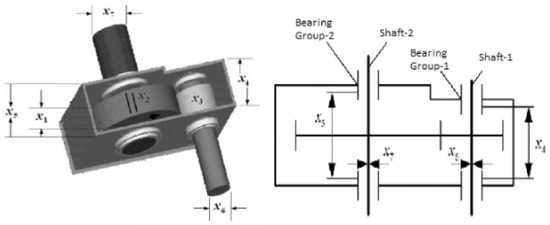
Figure 2. Speed reducer problem.

Table 17. Results of the speed reducer problem.

Algorithm	$\mathit{X}1$	$\mathit{X}2$	$\mathit{X}3$	$\mathit{X}4$	$\mathit{X}5$	$\mathit{X}6$	$\mathit{X}7$	Opt. Weight
MPAO	3.500	0.700	17.000	7.300	7.715322	3.350216	5.286655	2994.4725
CHHO [51]	3.500	0.700	17.000	7.300	7.715	3.350215	5.286655	2994.4737
HHO [51]	3.560	0.700	17.000	8.019	8.019	3.494800	5.286700	3060.3720
MDE [55]	3.500	0.700	17.000	7.300	7.800	3.350221	5.286685	2996.3566
PSO-DE [56]	3.500	0.700	17.000	7.300	7.800	3.350214	5.286683	2996.3481
PSO [57]	3.581	0.700	17.828	7.984	7.821	3.153980	5.187300	3005.3248
MBA [58]	3.500	0.700	17.000	7.300	7.716	3.350218	5.286654	2994.4824
SSA [57]	3.500	0.700	17.000	7.800	7.850	3.352470	5.286700	3002.5678
ISCA [57]	3.500	0.700	17.000	7.300	7.800	3.351290	5.286980	2997.1295

5.3.4. Gear Train Design Problem

Gear train is another kind of engineering optimization issue, which have four types of variables as shown in Figure 3. This kind of engineering issue aims to reduce the teeth ratio and the scaler value of the gear. Therefore, the decision parameter consists of the number of teeth on each gear.

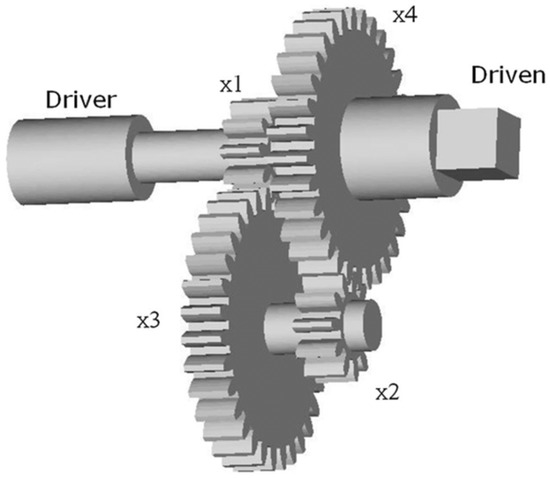
Figure 3. Gear train design problem.

To test the effect of the proposed MPAO algorithm in handling the problem of gear design, we compared to six optimization methods, including: CHHO [51], HHO [51], IMPFA [59], GeneAS [60], Kannan and Kramer [60], and Sandgren [60]. The test results of the proposed MPAO and other methods are listed in Table 18. The test result of the proposed MPAO algorithm is the best optimal value with 2.701E-12, which is followed by the IMPFA algorithm with 1.392E-10. Kannan and Kramer, GeneAS, and CHHO provided close results with 0.144121 for Kannan and Kramer, 0.144242 for GeneAS, and 0.1434 for CHHO. At the same time, HHO and Sandgren do not perform well, as they provide the lowest optimal value. The comparative results reveal that the proposed MPAO method is more precisely competent for handling the gear train design problem.

Table 18. Results of the gear train design problem.

Algorithm	$\mathit{X}1$	$\mathit{X}2$	$\mathit{X}3$	$\mathit{X}4$	Opt. Cost
MPAO	42.92	16.45	18.78	49.03	2.700 $\times {10}^{12}$
CHHO [51]	41.00	47.00	16.00	17.00	0.1434000
HHO [51]	56.00	58.00	22.00	21.00	0.14563000
IMPFA [59]	30.80	23.92	12.00	12.00	1.3915$\times {10}^{10}$
GeneAS [60]	50.00	33.00	14.00	17.00	0.14424200
Kannan and Kramer [60]	41.00	33.00	15.00	13.00	0.14412100
Sandgren [60]	60.00	45.00	22.00	18.00	0.14666700

To sum up, the outcomes of the previous experiments and the statistical analyses show that the proposed algorithm outperformed all others in obtaining the optimal outcomes and demonstrated its efficiency in most cases in solving FS, global optimization, and engineering problems. Evaluating the efficacy of MPAO relies on different performance metrics, including Min, Max, and Std of the fitness value, besides the classification accuracy, number of features, computation time, and Wilcoxon rank sum test. The MPAO showed some advantages, such as fast convergence, maintaining the search space with good exploration behavior, and escaping from the local optima in most cases. However, it showed a limitation in requiring a higher computation time, which needs to be improved in future study. In general, the better performance of the proposed MPAO can be due to the exploration’s improvement and exploitative capabilities, along with the utilization of AO parameters.

6. Conclusions

This study suggested an improved marine predators algorithm (MPA) efficient optimization technique for handling global optimization, feature selection (FS), and real-world engineering problems. The proposed algorithm in this paper used the strategy of the narrowed exploration of the Aquila optimizer (AO) to update the search space and explore more regions in the search domain to enhance the exploration behavior of the MPA. Therefore, the narrowed exploration of the AO increased the searchability of the MPA, thereby improving its ability to obtain the optimal or near-optimal results and thus helping the original MPA to overcome the local optima issues in the search domain effectively. The MPAO was evaluated for solving three problems: global optimization, feature selection, and real engineering cases. At first, the MPAO was evaluated on ten benchmark global optimization functions and outperformed the other algorithms in 60% of the functions. Concerning the FS experiment, a set of UCI datasets and four evaluation criteria were considered to prove the effectiveness of the suggested MPAO compared to nine metaheuristic optimization algorithms. Moreover, four engineering optimization issues were also considered to demonstrate the superiority of the suggested MPAO. The findings showed that the performance measures proved the superiority of the suggested MPAO compared to other methods in terms of Max, Min, and Std of the fitness function and accuracy over all considered FS issues. It outperformed the compared method in 87% of the datasets in terms of classification accuracy. The MPAO provided better results than the compared methods regarding real engineering problems. In the future, the proposed method will be used to solve more real-world problems, such as wind speed estimation, business optimization issues, and large-scale optimization problems.

References

- Kohavi, R.; John, G.H. Wrappers for feature subset selection. Artif. Intell. 1997, 97, 273–324. [Google Scholar] [CrossRef]
- Liu, H.; Motoda, H. Feature Extraction, Construction and Selection: A Data Mining Perspective; Springer Science & Business Media: Berlin/Heidelberg, Germany, 1998; Volume 453. [Google Scholar]
- Luukka, P. Feature selection using fuzzy entropy measures with similarity classifier. Expert Syst. Appl. 2011, 38, 4600–4607. [Google Scholar] [CrossRef]
- Talbi, E.G. Metaheuristics: From Design to Implementation; John Wiley & Sons: Hoboken, NJ, USA, 2009. [Google Scholar]
- Saremi, S.; Mirjalili, S.; Lewis, A. Grasshopper optimisation algorithm: Theory and application. Adv. Eng. Softw. 2017, 105, 30–47. [Google Scholar] [CrossRef]
- Hussien, A.G.; Amin, M. A self-adaptive Harris Hawks optimization algorithm with opposition-based learning and chaotic local search strategy for global optimization and feature selection. Int. J. Mach. Learn. Cybern. 2022, 13, 309–336. [Google Scholar] [CrossRef]
- Hashim, F.A.; Hussien, A.G. Snake Optimizer: A novel meta-heuristic optimization algorithm. Knowl.-Based Syst. 2022, 242, 108320. [Google Scholar] [CrossRef]
- Mostafa, R.R.; Hussien, A.G.; Khan, M.A.; Kadry, S.; Hashim, F.A. Enhanced coot optimization algorithm for dimensionality reduction. In Proceedings of the 2022 Fifth International Conference of Women in Data Science at Prince Sultan University (WiDS PSU), Riyadh, Saudi Arabia, 28–29 March 2022; pp. 43–48. [Google Scholar]
- Rao, R.V.; Savsani, V.J.; Vakharia, D. Teaching–learning-based optimization: A novel method for constrained mechanical design optimization problems. Comput.-Aided Des. 2011, 43, 303–315. [Google Scholar] [CrossRef]
- Ramezani, F.; Lotfi, S. Social-based algorithm (SBA). Appl. Soft Comput. 2013, 13, 2837–2856. [Google Scholar] [CrossRef]
- Atashpaz-Gargari, E.; Lucas, C. Imperialist competitive algorithm: An algorithm for optimization inspired by imperialistic competition. In Proceedings of the 2007 IEEE Congress on Evolutionary Computation, Singapore, 25–28 September 2007; pp. 4661–4667. [Google Scholar]
- Javidy, B.; Hatamlou, A.; Mirjalili, S. Ions motion algorithm for solving optimization problems. Appl. Soft Comput. 2015, 32, 72–79. [Google Scholar] [CrossRef]
- Abualigah, L.; Elaziz, M.A.; Hussien, A.G.; Alsalibi, B.; Jalali, S.M.J.; Gandomi, A.H. Lightning search algorithm: A comprehensive survey. Appl. Intell. 2021, 51, 2353–2376. [Google Scholar] [CrossRef]
- Doğan, B.; Ölmez, T. A new metaheuristic for numerical function optimization: Vortex Search algorithm. Inf. Sci. 2015, 293, 125–145. [Google Scholar] [CrossRef]
- Holland, J.H. Adaptation in Natural and Artificial Systems: An Introductory Analysis with Applications to Biology, Control, and Artificial Intelligence; MIT Press: Cambridge, MA, USA, 1992. [Google Scholar]
- Rocca, P.; Oliveri, G.; Massa, A. Differential evolution as applied to electromagnetics. IEEE Antennas Propag. Mag. 2011, 53, 38–49. [Google Scholar] [CrossRef]
- Passino, K.M. Biomimicry of bacterial foraging for distributed optimization and control. IEEE Control Syst. Mag. 2002, 22, 52–67. [Google Scholar]
- Moscato, P.; Mendes, A.; Berretta, R. Benchmarking a memetic algorithm for ordering microarray data. Biosystems 2007, 88, 56–75. [Google Scholar] [CrossRef] [PubMed]
- Wolpert, D.H.; Macready, W.G. No free lunch theorems for optimization. IEEE Trans. Evol. Comput. 1997, 1, 67–82. [Google Scholar] [CrossRef]
- Faramarzi, A.; Heidarinejad, M.; Mirjalili, S.; Gandomi, A.H. Marine Predators Algorithm: A nature-inspired metaheuristic. Expert Syst. Appl. 2020, 152, 113377. [Google Scholar] [CrossRef]
- Abualigah, L.; Yousri, D.; Abd Elaziz, M.; Ewees, A.A.; Al-qaness, M.A.; Gandomi, A.H. Aquila Optimizer: A novel meta-heuristic optimization Algorithm. Comput. Ind. Eng. 2021, 157, 107250. [Google Scholar] [CrossRef]
- Aribowo, W.; Supari, B.S.; Suprianto, B. Optimization of PID parameters for controlling DC motor based on the aquila optimizer algorithm. Int. J. Power Electron. Drive Syst. (IJPEDS) 2022, 13, 808–2814. [Google Scholar] [CrossRef]
- Hussan, M.R.; Sarwar, M.I.; Sarwar, A.; Tariq, M.; Ahmad, S.; Shah Noor Mohamed, A.; Khan, I.A.; Ali Khan, M.M. Aquila Optimization Based Harmonic Elimination in a Modified H-Bridge Inverter. Sustainability 2022, 14, 929. [Google Scholar] [CrossRef]
- Khaire, U.M.; Dhanalakshmi, R.; Balakrishnan, K. Hybrid Marine Predator Algorithm with Simulated Annealing for Feature Selection. In Machine Learning and Deep Learning in Medical Data Analytics and Healthcare Applications; CRC Press: Boca Raton, FL, USA, 2022; pp. 131–150. [Google Scholar]
- Alrasheedi, A.F.; Alnowibet, K.A.; Saxena, A.; Sallam, K.M.; Mohamed, A.W. Chaos Embed Marine Predator (CMPA) Algorithm for Feature Selection. Mathematics 2022, 10, 1411. [Google Scholar] [CrossRef]
- Balakrishnan, K.; Dhanalakshmi, R.; Mahadeo Khaire, U. Analysing stable feature selection through an augmented marine predator algorithm based on opposition-based learning. Expert Syst. 2022, 39, e12816. [Google Scholar] [CrossRef]
- Tizhoosh, H.R. Opposition-based learning: A new scheme for machine intelligence. In Proceedings of the International Conference on Computational Intelligence for Modelling, Control and Automation and International Conference on Intelligent Agents, Web Technologies and Internet Commerce (CIMCA-IAWTIC’06), Vienna, Austria, 28–30 November 2005; Volume 1, pp. 695–701. [Google Scholar]
- Abd Elaziz, M.; Ewees, A.A.; Yousri, D.; Abualigah, L.; Al-qaness, M.A. Modified marine predators algorithm for feature selection: Case study metabolomics. Knowl. Inf. Syst. 2022, 64, 261–287. [Google Scholar] [CrossRef]
- Jia, H.; Sun, K.; Li, Y.; Cao, N. Improved marine predators algorithm for feature selection and SVM optimization. KSII Trans. Internet Inf. Syst. (TIIS) 2022, 16, 1128–1145. [Google Scholar]
- Hu, G.; Zhu, X.; Wang, X.; Wei, G. Multi-strategy boosted marine predators algorithm for optimizing approximate developable surface. Knowl.-Based Syst. 2022, 254, 109615. [Google Scholar] [CrossRef]
- Hu, G.; Zhu, X.; Wei, G.; Chang, C.T. An improved marine predators algorithm for shape optimization of developable Ball surfaces. Eng. Appl. Artif. Intell. 2021, 105, 104417. [Google Scholar] [CrossRef]
- Han, M.; Du, Z.; Zhu, H.; Li, Y.; Yuan, Q.; Zhu, H. Golden-Sine dynamic marine predator algorithm for addressing engineering design optimization. Expert Syst. Appl. 2022, 210, 118460. [Google Scholar] [CrossRef]
- Al-qaness, M.A.; Ewees, A.A.; Fan, H.; Abualigah, L.; Abd Elaziz, M. Boosted ANFIS model using augmented marine predator algorithm with mutation operators for wind power forecasting. Appl. Energy 2022, 314, 118851. [Google Scholar] [CrossRef]
- Abdel-Basset, M.; Mohamed, R.; Abouhawwash, M. Hybrid marine predators algorithm for image segmentation: Analysis and validations. Artif. Intell. Rev. 2022, 55, 3315–3367. [Google Scholar] [CrossRef]
- Nadimi-Shahraki, M.H.; Taghian, S.; Mirjalili, S.; Abualigah, L. Binary Aquila Optimizer for Selecting Effective Features from Medical Data: A COVID-19 Case Study. Mathematics 2022, 10, 1929. [Google Scholar] [CrossRef]
- Abd Elaziz, M.; Dahou, A.; Alsaleh, N.A.; Elsheikh, A.H.; Saba, A.I.; Ahmadein, M. Boosting COVID-19 image classification using MobileNetV3 and aquila optimizer algorithm. Entropy 2021, 23, 1383. [Google Scholar] [CrossRef]
- Fatani, A.; Dahou, A.; Al-Qaness, M.A.; Lu, S.; Elaziz, M.A. Advanced feature extraction and selection approach using deep learning and Aquila optimizer for IoT intrusion detection system. Sensors 2021, 22, 140. [Google Scholar] [CrossRef]
- Zhang, Y.J.; Zhao, J.; Gao, Z.M. Hybridized improvement of the chaotic Harris Hawk optimization algorithm and Aquila Optimizer. In Proceedings of the International Conference on Electronic Information Engineering and Computer Communication (EIECC 2021), SPIE, Nanchang, China, 17–19 December 2021; Volume 12172, pp. 327–332. [Google Scholar]
- Wang, S.; Jia, H.; Abualigah, L.; Liu, Q.; Zheng, R. An improved hybrid aquila optimizer and harris hawks algorithm for solving industrial engineering optimization problems. Processes 2021, 9, 1551. [Google Scholar] [CrossRef]
- Kennedy, J.; Eberhart, R. Particle swarm optimization. In Proceedings of the ICNN’95-International Conference on Neural Networks, Western, Australia, 27 November–1 December 1995; Volume 4, pp. 1942–1948. [Google Scholar]
- Mitchell, M. An Introduction to Genetic Algorithms; MIT Press: Cambridge, MA, USA, 1998. [Google Scholar]
- Mirjalili, S. Moth-flame optimization algorithm: A novel nature-inspired heuristic paradigm. Knowl.-Based Syst. 2015, 89, 228–249. [Google Scholar] [CrossRef]
- Mirjalili, S.; Gandomi, A.H.; Mirjalili, S.Z.; Saremi, S.; Faris, H.; Mirjalili, S.M. Salp Swarm Algorithm: A bio-inspired optimizer for engineering design problems. Adv. Eng. Softw. 2017, 114, 163–191. [Google Scholar] [CrossRef]
- Li, S.; Chen, H.; Wang, M.; Heidari, A.A.; Mirjalili, S. Slime mould algorithm: A new method for stochastic optimization. Future Gener. Comput. Syst. 2020, 111, 300–323. [Google Scholar] [CrossRef]
- Mirjalili, S.; Lewis, A. The whale optimization algorithm. Adv. Eng. Softw. 2016, 95, 51–67. [Google Scholar] [CrossRef]
- Price, K.; Awad, N.; Ali, M.; Suganthan, P. The 100-Digit Challenge: Problem Definitions and Evaluation Criteria for the 100-Digit Challenge Special Session and Competition on Single Objective Numerical Optimization; Nanyang Technological University: Singapore, 2018. [Google Scholar]
- Wang, Y.; Li, H.X.; Huang, T.; Li, L. Differential evolution based on covariance matrix learning and bimodal distribution parameter setting. Appl. Soft Comput. 2014, 18, 232–247. [Google Scholar] [CrossRef]
- Gandomi, A.H.; Yang, X.S.; Alavi, A.H. Cuckoo search algorithm: A metaheuristic approach to solve structural optimization problems. Eng. Comput. 2013, 29, 17–35. [Google Scholar] [CrossRef]
- Mirjalili, S.; Mirjalili, S.M.; Lewis, A. Grey wolf optimizer. Adv. Eng. Softw. 2014, 69, 46–61. [Google Scholar] [CrossRef]
- Xing, Z.; Jia, H. Multilevel color image segmentation based on GLCM and improved salp swarm algorithm. IEEE Access 2019, 7, 37672–37690. [Google Scholar] [CrossRef]
- Dhawale, D.; Kamboj, V.K.; Anand, P. An improved chaotic harris hawks optimizer for solving numerical and engineering optimization problems. Eng. Comput. 2021, 1–46. [Google Scholar] [CrossRef]
- Kamboj, V.K.; Bhadoria, A.; Gupta, N. A novel hybrid GWO-PS algorithm for standard benchmark optimization problems. INAE Lett. 2018, 3, 217–241. [Google Scholar] [CrossRef]
- Mirjalili, S.; Mirjalili, S.M.; Hatamlou, A. Multi-verse optimizer: A nature-inspired algorithm for global optimization. Neural Comput. Appl. 2016, 27, 495–513. [Google Scholar] [CrossRef]
- Savsani, P.; Savsani, V. Passing vehicle search (PVS): A novel metaheuristic algorithm. Appl. Math. Model. 2016, 40, 3951–3978. [Google Scholar] [CrossRef]
- Zhao, W.; Zhang, Z.; Wang, L. Manta ray foraging optimization: An effective bio-inspired optimizer for engineering applications. Eng. Appl. Artif. Intell. 2020, 87, 103300. [Google Scholar] [CrossRef]
- Niu, B.; Li, L. A novel PSO-DE-based hybrid algorithm for global optimization. International Conference on Intelligent Computing; Springer: Berlin/Heidelberg, Germany, 2008; pp. 156–163. [Google Scholar]
- Gupta, S.; Deep, K.; Moayedi, H.; Foong, L.K.; Assad, A. Sine cosine grey wolf optimizer to solve engineering design problems. Eng. Comput. 2021, 37, 3123–3149. [Google Scholar] [CrossRef]
- Sadollah, A.; Bahreininejad, A.; Eskandar, H.; Hamdi, M. Mine blast algorithm: A new population based algorithm for solving constrained engineering optimization problems. Appl. Soft Comput. 2013, 13, 2592–2612. [Google Scholar] [CrossRef]
- Tang, C.; Zhou, Y.; Luo, Q.; Tang, Z. An enhanced pathfinder algorithm for engineering optimization problems. Eng. Comput. 2022, 38, 1481–1503. [Google Scholar] [CrossRef]
- Deb, K.; Goyal, M. A combined genetic adaptive search (GeneAS) for engineering design. Comput. Sci. Inform. 1996, 26, 30–45. [Google Scholar]
Publisher’s Note: MDPI stays neutral with regard to jurisdictional claims in published maps and institutional affiliations. |
© 2022 by the authors. Licensee MDPI, Basel, Switzerland. This article is an open access article distributed under the terms and conditions of the Creative Commons Attribution (CC BY) license (https://creativecommons.org/licenses/by/4.0/).