Existence and Uniqueness of a Curve with Both Minimal Length and Minimal Area

Abstract

Consider the family of generalized parabolas $\{y=-a{x}^r+c|a,r,c,x>0,r\mathrm{is}\mathrm{a}\mathrm{fixed}\mathrm{constant}\}$ that pass through a given point in the first quadrant (and hence, depend on one parameter only). Find the parameter values for which the piece of the corresponding parabola in the first quadrant either encloses a minimum area, or has a minimum length. We find a sufficient condition under which given the fixed point, the area minimizing curve and the length minimizing curve coincide. The problem led us to a certain implicit function and we explored its asymptotic behavior and convexity.

1. Introduction

Optimization problems with geometrical constraints are well studied and can be solved in different approaches, e.g., by giving an algorithmic approximation, a numerical solution or an analytic solution. One often needs to prove analytically that the solution exists, and then uniqueness comes into question. Although such problems in the plane are easy to define and understand, the solution is often non-trivial and requires a great deal of effort to achieve. Our problem is inspired by several other problems in the plane. Ref. [1] presents a method to obtain a minimal covering of a thin convex domain, based on minimizing the area of the respective Minkowski sum. Ref. [2] defines an algorithm which approximates the minimal area encasing rectangle for an arbitrary closed curve, it first determines the minimal perimeter and then selects the area of the minimal rectangle which contains the polygon. Ref. [3] describes how to reconstruct a curve that is partially hidden or corrupted by minimizing the functional $\int \sqrt{1+K^2}ds$, depending both on the length and curvature K. It turns out that minimization of curves by length and curvature can lead to character recognition, prototype formation, and object recognition, and is potentially useful in other applications such as registration and tracking, for more details see [4]. Refs. [5,6] described an algorithm for computing the minimum enclosing circle or ellipse of a set of planar curves, in the case of a circle the expected running time is linear in the number of input curves. Ref. [7] provides us with uniqueness results for minimal volume enclosing ellipsoids in d dimensions.

The problem of finding the minimum perimeter bounding shape has also been considered before. Ref. [8] discussed the computation of minimum perimeter triangle enclosing a convex polygon. Ref. [9] gave a polynomial-time algorithm for the problem of finding a minimum-perimeter k-gon that encloses a given n-gon. Given n points in the plane, Ref. [10] showed way to compute various enclosing isosceles triangles where different parameters such as area or perimeter are optimized. A problem in the plane which involves both area and length has been formulated by Santaló and solved in [11], which determines analytically the planar convex sets which have maximum and minimum area or perimeter when the circumradius and the inradius are given.

These and other similar problems have risen some questions. What if we consider minimizing the enclosing shapes’ area and perimeter simultaneously? What other enclosing shapes can we consider which possess some property of existence and uniqueness?

Our problem is inspired by tunnel construction. Suppose that we are tasked with building a road tunnel that passes through a mountain and must accommodate the size of some truck. We might want to optimize some variables such us the amount of soil that must be dug or the surface area of the tunnel’s ceiling. It is expected that it is possible to completely optimize the tunnel with respect to only one of these variables. The question that rises is whether it is possible for the tunnel that minimizes the amount of soil that must be dug to be the same as the tunnel with minimal ceiling surface area. If so, then what sort of tunnels would have to be considered? What would the truck’s measurements be? Suppose the possible outlines of the tunnels are given by a family of curves. We model the truck by a rectangle with width $2k$ and height t. We place the rectangle on the x-axis and pass the y-axis through its center. Since the tunnels are probably symmetric, we can assume our family consists of symmetric curves and shift our focus to the first quadrant. The top right corner of the rectangle is the point $(k,t)$ and since we are interested in optimal solutions we impose that the curves must pass through that point. We assume that the curves intersect the $x,y$-axes and that they enclose the rectangle. Minimizing the area bounded between the curves and the $x,y$-axes corresponds to minimizing the amount of soil that must be dug, and minimizing the arc length between the intersection points with the $x,y$-axes corresponds to minimizing the surface area of the tunnel’s ceiling. We chose to study the family

$$\{y=-a{x}^r+c|a,r,c,x>0,r\mathrm{is}\mathrm{a}\mathrm{fixed}\mathrm{constant}\}.$$

We found this family to be an adequate exploration starting point, since it surprisingly posses nice properties which lead to a rigorous analytical proof of the solution. For $0<r<1$ the family does not resemble tunnels since the curves would be concave, but for $r>1$ there is a clear resemblance, as can be seen in Figure 1.

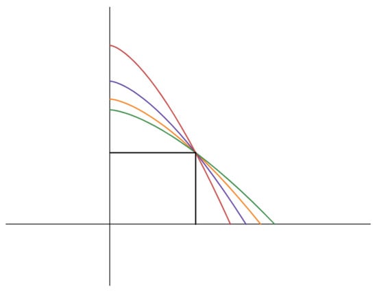
Figure 1. An illustration of the problem’s setup, where the rectangle’s width is $k=2.4$, the height is $t=2$ and the degree of the family $r=1.5$. Each curve defines the area and curve length.

Given the rectangle’s width, we show that there exists a height such the curve which minimizes the area and the curve which minimizes the length coincide (see Figure 2 for an example).

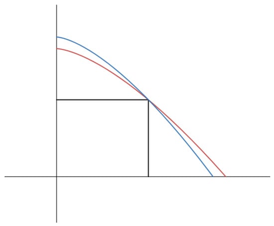
Figure 2. With the same parameters as in Figure fig:family, the curve in blue with $a\approx 0.44$ minimizes the length and the curve in red with $a=\frac{10}{3}$ minimizes the area. Usually these two curves do not coincide.

2. Preliminaries

First we give a formulation of the desired definitions and theorems. Let $k,t,r>0$$k,t,r\in {\mathbb{R}}^{+}$ be constants.

Definition 1.

Let A be the family of curves in ${\mathbb{R}}^2$ defined by:

$$A=\{y_{a,c}\left(x\right)=-a{x}^r+c|a,c,x,r>0\}$$

Definition 2.

Denote by B the family of curves in A which pass through a given point $(k,t)$ with $c>t$ (see Figure 1).

The constraint in Definition 2 makes the family of curves B depend on one parameter only. The algebraic relation between a and c is

$$-a{k}^r+c=t\iff c=t+a{k}^r\iff a=\frac{c-t}{k^r}.$$

(1)

Definition 3.

We define $p>0$ to be the x-coordinate of the point of intersection of a curve in B with the x-axis.

The algebraic expression for p can be easily obtained:

$$-a{p}^r+c=0⟹p={\left(\frac{c}{a}\right)}^{1/r}={\left(\frac{t+a{k}^r}{a}\right)}^{1/r}=k{\left(\frac{c}{c-t}\right)}^{1/r}.$$

(2)

Remark 1.

The variable p could be represented as a function of a or c. When we write p and do not follow it with parentheses, it should be understood by context whether we mean it as a function of a or c.

Remark 2.

When we say “find the curve” we mean find the variables a and c which determine it. It is enough to find an expression for either a or c.

Recall the following theorems which will later be used:

Theorem 1

(Leibniz Integral Rule; [12], p. 307, Thm. 23.11). Let $f\left(x,y\right)$ be defined on the rectangle $[a,b]\times [\alpha ,\beta ]$. If f and $\frac{\partial f}{\partial y}$ are continuous and the functions $a\left(y\right),b\left(y\right)$ are differentiable on $[\alpha ,\beta ]$, then $\frac{d}{dy}{\int }_{a\left(y\right)}^{b\left(y\right)}f\left(x,y\right)dx$ exists and is expressible as:

$$\frac{d}{dy}{\int }_{a\left(y\right)}^{b\left(y\right)}f\left(x,y\right)dx={\int }_{a\left(y\right)}^{b\left(y\right)}\frac{\partial f}{\partial y}\left(x,y\right)dx+f\left(b\left(y\right),y\right)b^{\prime }\left(y\right)-f\left(a\left(y\right),y\right)a^{\prime }\left(y\right).$$

Theorem 2

([13], p.18, Thm. 11). Let $f(x,y)$ and $\frac{\partial f}{\partial y}$$f_y$ be continuous on $(a,b]\times [c,d]$. Suppose that the improper integral:

$$F\left(y\right)={\int }_a^{b}f\left(x,y\right)dx$$

converges for some $y_0\in [c,d]$ and:

$$G\left(y\right)={\int }_a^b\frac{\partial f}{\partial y}\left(x,y\right)dx$$

converges uniformly on $[c,d]$. Then F converges uniformly on $[c,d]$ and it is continuously differentiable on $[c,d]$; specifically,

$$F^{\prime }\left(y\right)=G\left(y\right).$$

Theorem 3

(Generalized Binomial Theorem). If $r\in \mathbb{R}$ and $\left|x\right|<\left|y\right|$, then:

$${(x+y)}^r=\sum _{k=0}^{\infty }\left(\genfrac{}{}{0pt}{}{r}{k}\right)x^k{y}^{r-k},$$

where $\left(\genfrac{}{}{0pt}{}{r}{k}\right)$ follows the same recurrence relation as the regular binomial coefficient, i.e., $\left(\genfrac{}{}{0pt}{}{r}{0}\right)=1$ and $\left(\genfrac{}{}{0pt}{}{r}{k+1}\right)=\left(\genfrac{}{}{0pt}{}{r}{k}\right)\frac{r-k}{k+1}.$

Theorem 4

([13], p.15, Thm. 10). Let $J=[\alpha ,\beta ]$. If $f:(a,b]\times J\to \mathbb{R}$ is continuous and the improper integral

$$F\left(t\right)={\int }_a^{b}f(x,t)dx=\underset{c\to a+}{lim}{\int }_c^{b}f(x,t)dx$$

is uniformly convergent for $t\in J$, then $F:J\to \mathbb{R}$ is continuous on J.

3. Minimizing the Area

In this section, we focus on finding the curve in B which minimizes the area in the first quadrant bounded between the curves in B and the $x,y$-axes. The results here are necessary for later sections where we minimize both area and length. It is apparent that when minimizing the area it is convenient to leave the dependency on c and represent a as a function of c.

Lemma 1.

The desired area is obtained by

$$A\left(c\right)=\frac{rcp}{r+1}$$

where p in the intersection of the curve with the x-axis.

Proof. 

$$\begin{array}{cc}\hfill A\left(c\right)& ={\int }_0^p\left(-a{x}^r+c\right)dx=\frac{-a{p}^{r+1}}{r+1}+cp=\frac{-a{p}^{r+1}+cp\left(r+1\right)}{r+1}=\hfill \\ & =\frac{p\left(-a{p}^r+c\left(r+1\right)\right)}{r+1}\stackrel{\left(2\right)}{=}\frac{p\left(-a{\left(\frac{c}{a}\right)}^{\frac{r}{r}}+c\left(r+1\right)\right)}{r+1}=\frac{rcp}{r+1}\hfill \end{array}$$

□

We get a one dimensional optimization problem, which leads to the following Lemma.

Lemma 2.

The derivative of $A\left(c\right)$ is

$$A^{\prime }\left(c\right)=\frac{k{c}^{1/r}\left(rc-rt-t\right)}{\left(r+1\right){\left(c-t\right)}^{1/r+1}}.$$

Proof. 

Since $p\left(c\right)=k{\left(\frac{c}{c-t}\right)}^{1/r}$, then

$$\frac{dp}{dc}=\frac{d}{dc}k{\left(\frac{c}{c-t}\right)}^{1/r}=-\frac{kt{c}^{1/r-1}}{r{\left(c-t\right)}^{1/r+1}}.$$

(3)

Afterwards:

$$\begin{array}{cc}\hfill A^{\prime }\left(c\right)& \stackrel{\left(1\right)}{=}\frac{d}{dc}\left(\frac{rcp}{r+1}\right)=\frac{r}{r+1}\left(p+c\frac{dp}{dc}\right)\stackrel{\left(3\right)}{=}\hfill \\ \hfill & =\frac{r}{r+1}\left(k{\left(\frac{c}{c-t}\right)}^{1/r}-\frac{kt{c}^{1/r}}{r{\left(c-t\right)}^{1/r+1}}\right)=\frac{k{c}^{1/r}\left(rc-rt-t\right)}{\left(r+1\right){\left(c-t\right)}^{1/r+1}}.\hfill \end{array}$$

□

Theorem 5.

There exists a unique curve which minimizes $A\left(c\right)$.

Proof. 

From Lemma 2, we obtain that $A^{\prime }\left(c\right)=0\iff c=c_0=\frac{\left(r+1\right)t}{r}$.

In addition, for all $c\in \left(0,c_0\right),A^{\prime }\left(c\right)<0$ and for all $c\in \left(c_0,\infty \right),A^{\prime }\left(c\right)>0$. Therefore, $A\left(c\right)$ has its global minimum at $c_0$ and it is only attained there. □

Corollary 1.

The curve $y\in B$ which minimizes the area is given by: $y=-a{x}^r+c$, where $c=\frac{\left(r+1\right)t}{r}$, and by (1) we get $a=\frac{t}{r{k}^r}$.

4. Minimizing the Length

Definition 4.

Define $L:{\mathbb{R}}^{+}\to {\mathbb{R}}^{+}$ to be the function that receives the parameter a of a curve in B and returns the length of the curve from its intersection with the y-axis to its intersection with the x-axis.

Recall that the formula for the length of a curve $y=f\left(x\right)$ in the Cartesian plane from $x=a$ to $x=b$ is:

$${\int }_a^b\sqrt{1+{\left(\frac{dy}{dx}\right)}^2}dx$$

(4)

In our case, we get:

$$\frac{dy}{dx}=\frac{d}{dx}(-a{x}^r+c)=-ar{x}^{r-1}$$

(5)

Using (4) and (5), our expression for $L\left(a\right)$ is:

$$L\left(a\right)={\int }_0^p\sqrt{1+{(-ar{x}^{r-1})}^2}dx={\int }_0^p\sqrt{1+{\left(ar{x}^{r-1}\right)}^2}dx$$

(6)

Figure 3 shows a typical graph of $L\left(a\right)$, giving us insight into its properties.

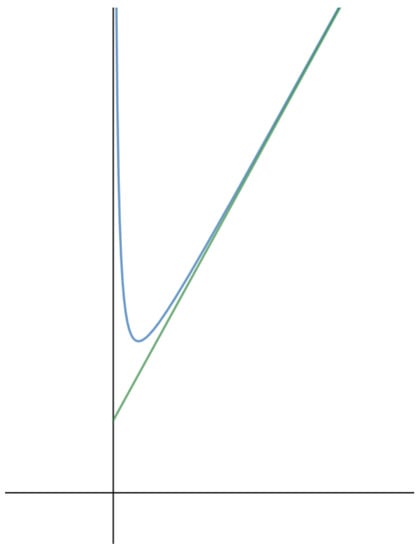
Figure 3. A typical graph of $L\left(a\right)$, along with $t+a{k}^r$ which appears to be asymptotic to it. $L\left(a\right)$ appears to be continuous, strictly convex and to approach $+\infty$ as $a\to 0^{+}$ and as $a\to +\infty$.

In a similar way to the area formulation, we first show that there exists a unique curve which minimizes the length.

Lemma 3.

$L\left(a\right)\to +\infty$ as $a\to 0^{+}$

Proof. 

Using the criteria for infinite limits comparison:

$$\begin{array}{cc}\hfill & \underset{a\to 0^{+}}{lim}L\left(a\right)\stackrel{\left(6\right)}{=}\underset{a\to 0^{+}}{lim}{\int }_0^p\sqrt{1+{\left(ar{x}^{r-1}\right)}^2}dx\ge \underset{a\to 0^{+}}{lim}{\int }_0^p\sqrt{1}dx=\hfill \\ \hfill =& \underset{a\to 0^{+}}{lim}p\stackrel{\left(2\right)}{=}\underset{a\to 0^{+}}{lim}{\left(\frac{t+a{k}^r}{a}\right)}^{1/r}=+\infty \hfill \end{array}$$

$$⟹\underset{a\to 0^{+}}{lim}L\left(a\right)=+\infty$$

□

Lemma 4.

$L\left(a\right)\to +\infty$ as $a\to +\infty$

Proof. 

Using the criteria for infinite limits comparison:

$$\begin{array}{cc}\hfill \underset{a\to +\infty }{lim}L\left(a\right)& \stackrel{\left(6\right)}{=}\underset{a\to +\infty }{lim}{\int }_0^p\sqrt{1+{\left(ar{x}^{r-1}\right)}^2}dx\ge \underset{a\to +\infty }{lim}{\int }_0^{p}ar{x}^{r-1}dx=\hfill \\ \hfill & =\underset{a\to +\infty }{lim}a{p}^r\stackrel{\left(2\right)}{=}\underset{a\to +\infty }{lim}c\stackrel{\left(1\right)}{=}\underset{a\to +\infty }{lim}t+a{k}^r=+\infty \hfill \end{array}$$

$$⟹\underset{a\to \infty }{lim}L\left(a\right)=+\infty$$

□

For $r\ge 1$ our integral in the formula for $L\left(a\right)$ is a proper integral, but for $0<r<1$ our integral is improper, so we often need to separate our proofs into two cases, as in the following lemma.

Lemma 5.

$L\left(a\right)$ is differentiable on $\left(0,\infty \right)$.

Proof. 

We consider 2 separate cases:

Case 1: Assume $r\ge 1$

$$L\left(a\right)={\int }_0^p\sqrt{1+{\left(ar{x}^{r-1}\right)}^2}dx$$

Denote

$$\begin{array}{c}\hfill z(a,x)=\sqrt{1+{\left(ar{x}^{r-1}\right)}^2},\end{array}$$

(7)

$z(a,x)$ and $\frac{\partial z}{\partial a}=\frac{{\left(ar{x}^{r-1}\right)}^2}{a\sqrt{1+{\left(ar{x}^{r-1}\right)}^2}}$ are continuous. In addition, our bounds, 0 and $p={\left(\frac{t+a{k}^r}{a}\right)}^{1/r}$ are differentiable with respect to a, so by Theorem 1, $L^{\prime }\left(a\right)$ exists.

Case 2: Assume $0<r<1$. We write:

$${\int }_0^{p}z\left(a,x\right)dx={\int }_0^{k}z\left(a,x\right)dx+{\int }_k^{p}z\left(a,x\right)dx$$

The integral ${\int }_k^{p}z\left(a,x\right)dx$ is differentiable by Theorem 1. To prove ${\int }_0^{k}z\left(a,x\right)dx$ is differentiable, we recall Theorem 2. Let $a_0\in (0,\infty )$. Choose an interval $[c,d]$ such that $[c,d]\subset (0,\infty )$ and $c<a_0<d$. The integral:

$${\int }_0^k\sqrt{1+{\left(ar{x}^{r-1}\right)}^2}dx$$

converges for all $a\in [c,d]$ by the limit comparison test with $x^{r-1}$ which converges since $r-1>0$. In addition, ${\int }_0^k\frac{\partial z}{\partial a}\left(a,x\right)dx$ converges uniformly by the Weierstrass M-test, since:

$$\left|\frac{\partial z}{\partial a}\right|=\frac{{\left(ar{x}^{r-1}\right)}^2}{a\sqrt{1+{\left(ar{x}^{r-1}\right)}^2}}\le \frac{d^2}{c^2}r{x}^{r-1}$$

and ${\int }_0^k\frac{d^2}{c^2}r{x}^{r-1}dx$ converges. As a result, by Theorem 2, ${\int }_0^{k}z\left(a,x\right)dx$ is differentiable with respect to a on $[c,d]$, and in particular at $a=a_0$. Since $a_0$ was arbitrary we can conclude that ${\int }_0^{k}z\left(a,x\right)dx$ is differentiable on $(0,\infty )$, and $L\left(a\right)$ is differentiable on $(0,\infty )$ as a sum of two differentiable functions. □

Lemma 6.

$L\left(a\right)$ is continuous on $(0,\infty )$.

Proof. 

By Lemma 5, $L\left(a\right)$ is differentiable and thus it is continuous on $(0,\infty )$. □

Lemma 7.

$L^{″}\left(a\right)>0$ for all $a\in (0,\infty )$

Proof. 

In the proof of Lemma 5 we saw that Theorem 1 can be applied:

$$L\left(a\right)={\int }_0^{p}z\left(a,x\right)dx⟹L^{\prime }\left(a\right)={\int }_0^p\frac{\partial z}{\partial a}\left(a,x\right)dx+\frac{dp}{da}·z\left(a,p\right).$$

It is easy to check that

$$\frac{{\partial }^{2}z}{\partial a^2}=\frac{{\left(r{x}^{r-1}\right)}^2}{{\left(1+{\left(ar{x}^{r-1}\right)}^2\right)}^{\frac{3}{2}}}$$

(8)

is also continuous, thus we can apply Theorem 1 again:

$$L^{″}\left(a\right)={\int }_0^p\frac{{\partial }^{2}z}{\partial a^2}\left(a,x\right)dx+\frac{dp}{da}·\frac{\partial z}{\partial a}\left(a,p\right)+\frac{d^{2}p}{d{a}^2}·z\left(a,p\right)+\frac{d}{da}\left(z\left(a,p\right)\right)·\frac{dp}{da}$$

Denote

$$U\left(a\right)=\frac{dp}{da}·\frac{\partial z}{\partial a}\left(a,p\right)+\frac{d^{2}p}{d{a}^2}·z\left(a,p\right)+\frac{d}{da}\left(z\left(a,p\right)\right)·\frac{dp}{da}=\frac{d^{2}p}{d{a}^2}z\left(a,p\right)+\frac{dp}{da}\left(\frac{d}{da}z\left(a,p\right)+\frac{\partial z}{\partial a}\left(a,p\right)\right)$$

Looking at (8), we see that for all $a>0$, $\frac{{\partial }^{2}z}{\partial a^2}>0$ and we know that $p>0$ so we can bound $L^{″}\left(a\right)$ from below with $U\left(a\right)$. We now prove that for all $a>0$, $U\left(a\right)>0$. We start by finding all the derivatives in the expression. Using the relation $p\left(a\right)={\left(\frac{t+a{k}^r}{a}\right)}^{\frac{1}{r}}$ and expression (7), we obtain:

$$z\left(a,p\right)=\sqrt{1+{\left(ar{p}^{r-1}\right)}^2}$$

$$\frac{dp}{da}=\frac{-tp}{ra\left(t+a{k}^r\right)}$$

$$\frac{\partial z}{\partial a}\left(a,p\right)=\frac{{\left(ar{p}^{r-1}\right)}^2}{a\sqrt{1+{\left(ar{p}^{r-1}\right)}^2}}$$

$$\frac{\partial z}{\partial x}\left(a,p\right)=\frac{\left(r-1\right){\left(ar{p}^{r-1}\right)}^2}{p\sqrt{1+{\left(ar{p}^{r-1}\right)}^2}}$$

$$\frac{d^{2}p}{d{a}^2}=\frac{tp\left(2ra{k}^r+t+rt\right)}{{\left((t+a{k}^r)ar\right)}^2}$$

In addition, using the chain rule:

$$\frac{d}{da}\left(z(a,p)\right)=\frac{\partial z}{\partial a}\left(a,p\right)+\frac{\partial z}{\partial x}\left(a,p\right)·\frac{dp}{da}$$

Substituting all these expressions and simplifying we get:

$$U\left(a\right)=\frac{tp\left(t+rt+2ra{k}^r\right)}{{\left((t+a{k}^r)ar\right)}^2\sqrt{1+{\left(ar{p}^{\left(r-1\right)}\right)}^2}}>0.$$

□

Theorem 6.

There exists a unique curve which minimizes $L\left(a\right)$.

Proof. 

Using Lemma 3, by the limit definition, there exists a number $\gamma \in (0,1)$ such that for all $a\in (0,\gamma )$, $L\left(a\right)>L\left(1\right)$. Similarly, using Lemma 4, there exists $\delta \in (1,\infty )$ such that for all $a\in (\delta ,\infty )$, $L\left(a\right)>L\left(1\right)$. Using Lemma 6 and Weierstrass extreme value theorem, $L\left(a\right)$ attains a minimum value on $[\gamma ,\delta ]$, at some point $(\beta ,m)$. Note that $m\le L\left(1\right)$ because $1\in [\gamma ,\delta ]$. Now, looking at the whole interval $(0,\infty )$:

• if $a\in (0,\gamma )$, then $L\left(a\right)>L\left(1\right)\ge m$
• if $a\in [\gamma ,\delta ]$, then $L\left(a\right)\ge m$
• if $a\in (\delta ,\infty )$, then $L\left(a\right)>L\left(1\right)\ge m$

Hence L has a global minimum. Lemma 7 implies that L is strictly convex and strictly convex functions have at most one global minimum. □

As to actually finding the a which minimizes $L\left(a\right)$, we solve the equation $L^{\prime }\left(a\right)=0$. Usually, it is not easy to find a closed form expression for $L^{\prime }\left(a\right)$. However, in the worst case, we can express it with an infinite sum and get a good approximation by taking a finite number of terms from the start. After approximating $L^{\prime }\left(a\right)$, we can solve for its root numerically. When choosing a numerical method, we have to take into consideration that $L^{\prime }\left(a\right)$ is only defined for $a>0$. We explore the following cases:

• $r=1$
• $r=2$
• $r>1$
• $0<r<1$

After analyzing each case, these are the result we have obtained, respectively:

• We have a closed form for $L\left(a\right)$, $L^{\prime }\left(a\right)$ and the root.
• We have a closed form for $L\left(a\right)$ and $L^{\prime }\left(a\right)$.
• We have a closed form for $L^{\prime }\left(a\right)$ for $r\in P_1=\{1+\frac{1}{2g}|g\in \mathbb{N}\}=\{1.5,1.25,1\frac{1}{6},1.125,$$1.1,\dots \}$ and an expression for $L^{\prime }\left(a\right)$ containing an infinite sum for $r\notin P_1$.
• We have a closed form for $L^{\prime }\left(a\right)$ for $r\in P_2=\{1-\frac{1}{2g}|g\in \mathbb{N}\}=\{0.5,0.75,\frac{5}{6},0.875,0.9,$$\dots \}$ and an expression for $L^{\prime }\left(a\right)$ containing an infinite sum for $r\notin P_2$.

4.1. The Case r = 1

For $r=1$, our curves are just straight lines from the points $(0,c)$ to the points $(p,0)$, as illustrated in Figure 4.

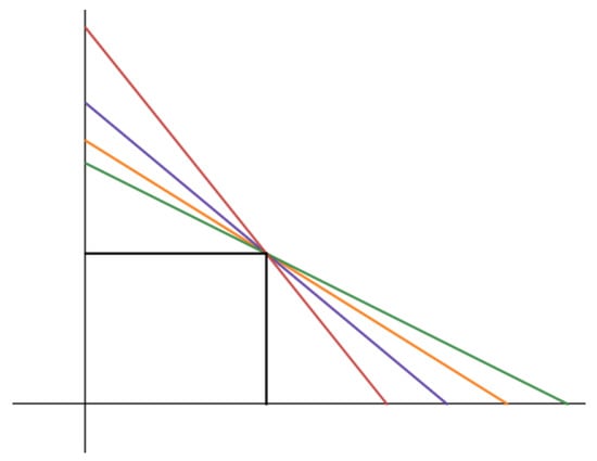
Figure 4. An example of four feasible curves when $r=1$.

Using the Pythagorean Theorem, our expression for the length is:

$$L\left(a\right)=\sqrt{c^2+p^2}=\sqrt{c^2+\frac{c^2}{a^2}}=c\sqrt{1+\frac{1}{a^2}}=\left(t+ak\right)\sqrt{1+\frac{1}{a^2}}$$

$$L^{\prime }\left(a\right)=k\sqrt{1+\frac{1}{a^2}}+\frac{-2\left(t+ak\right)}{2a^3\sqrt{1+\frac{1}{a^2}}}=\frac{k\left(1+\frac{1}{a^2}\right)a^3-t-ak}{a^3\sqrt{1+\frac{1}{a^2}}}=\frac{k{a}^3-t}{a^3\sqrt{1+\frac{1}{a^2}}}$$

Setting $L^{\prime }\left(a\right)=0$ we get:

$$a=a_0=\sqrt[3]{\frac{t}{k}}$$

For all $a\in \left(0,a_0\right)$, $L^{\prime }\left(a\right)<0$ and for all $a\in \left(a_0,\infty \right)$, $L^{\prime }\left(a\right)>0$ so the minimum is at $a_0$.

4.2. The Case r = 2

For $r=2$ we get:

$$L\left(a\right)={\int }_0^p\sqrt{1+{\left(ar{x}^{r-1}\right)}^2}={\int }_0^p\sqrt{1+{\left(2ax\right)}^2}$$

Making a change of variables:

$$tan\left(\theta \right)=2ax⟹sec\left(\theta \right)=\sqrt{1+{tan}^2\left(\theta \right)}=\sqrt{1+{\left(2ax\right)}^2}$$

$${sec}^2\left(\theta \right)d\theta =2adx⟹dx=\frac{{sec}^2\left(\theta \right)d\theta }{2a}$$

We first find the indefinite integral. Changing x to $\theta$ we get:

$$\int \frac{1}{2a}\sqrt{1+{tan}^2\left(\theta \right)}{sec}^2\left(\theta \right)d\theta =\frac{1}{2a}\int \sqrt{{sec}^2\left(\theta \right)}{sec}^2\left(\theta \right)d\theta =$$

$$=\frac{1}{2a}\int {sec}^3\left(\theta \right)d\theta =\frac{1}{2a}\left(\frac{1}{2}sec\left(\theta \right)tan\left(\theta \right)+\frac{1}{2}ln\left(tan\left(\theta \right)+sec(\theta \right))\right)$$

$$=\frac{1}{2a}\left(\frac{1}{2}2ax\sqrt{1+{\left(2ax\right)}^2}+\frac{1}{2}ln\left(2ax+\sqrt{1+{\left(2ax\right)}^2}\right)\right)+\mathrm{Const}.=$$

$$=\frac{1}{2}x\sqrt{1+{\left(2ax\right)}^2}+\frac{1}{4a}ln\left(2ax+\sqrt{1+{\left(2ax\right)}^2}\right)+\mathrm{Const}.$$

Substituting our bounds we get:

$$L\left(a\right)=\frac{p}{2}\sqrt{1+{\left(2ap\right)}^2}+\frac{1}{4a}ln\left(2ap+\sqrt{1+{\left(2ap\right)}^2}\right)$$

It is possible to differentiate $L\left(a\right)$. Note that p is a function of a, so the chain rule will have to be used.

4.3. The Case r ≠ 1

For $r\ne 1$, we will not express $L\left(a\right)$, but rather immediately express $L^{\prime }\left(a\right)$. We develop an expression for $L^{\prime }\left(a\right)$ based on Leibniz integral rule.

$$L^{\prime }\left(a\right)=\frac{d}{da}{\int }_0^p\sqrt{1+{\left(ar{x}^{r-1}\right)}^2}dx={\int }_0^p\frac{\partial }{\partial a}\sqrt{1+{\left(ar{x}^{r-1}\right)}^2}dx+\frac{dp}{da}\sqrt{1+{\left(ar{p}^{r-1}\right)}^2}$$

We find $\frac{dp}{da}$ and the partial derivative separately:

$$\frac{dp}{da}=\frac{d}{da}{\left(\frac{t+a{k}^r}{a}\right)}^{1/r}=\frac{-t{\left(t+a{k}^r\right)}^{1/r-1}}{r{a}^{1/r+1}}=\frac{-tp}{ra\left(t+a{k}^r\right)}$$

$$\frac{\partial }{\partial a}\sqrt{1+{\left(ar{x}^{r-1}\right)}^2}=\frac{2a{\left(r{x}^{r-1}\right)}^2}{2\sqrt{1+a^2{\left(r{x}^{r-1}\right)}^2}}=\frac{{\left(ar{x}^{r-1}\right)}^2}{a\sqrt{1+{\left(ar{x}^{r-1}\right)}^2}}$$

Now we are left with finding:

$$I={\int }_0^p\frac{{\left(ar{x}^{r-1}\right)}^2}{a\sqrt{1+{\left(ar{x}^{r-1}\right)}^2}}dx=\frac{1}{a}{\int }_0^p\frac{{\left(ar{x}^{r-1}\right)}^2}{\sqrt{1+{\left(ar{x}^{r-1}\right)}^2}}dx$$

Substitute:

$$v=ar{x}^{r-1}⟹x={\left(\frac{v}{ar}\right)}^{\frac{1}{r-1}}⟹dx=\frac{v^{\frac{1}{r-1}-1}}{\left(r-1\right){\left(ar\right)}^{\frac{1}{r-1}}}dv$$

$$⟹I=\frac{1}{a\left(r-1\right){\left(ar\right)}^{\frac{1}{r-1}}}{\int }_{v\left(0^{+}\right)}^{v\left(p\right)}\frac{v^{\frac{r}{r-1}}}{\sqrt{1+v^2}}dv$$

Substitute:

$$y=\sqrt{1+v^2}\iff y^2=1+v^2\iff v^2=y^2-1\iff v^{\frac{1}{r-1}}={\left(y^2-1\right)}^{\frac{1}{2\left(r-1\right)}}$$

$$⟹2ydy=2vdv⟹dv=\frac{\sqrt{1+v^2}}{v}dy.$$

which leads to

$$\begin{array}{c}\hfill I=\frac{1}{a\left(r-1\right){\left(ar\right)}^{\frac{1}{r-1}}}{\int }_{y\left(v\left(0^{+}\right)\right)}^{y\left(v\left(p\right)\right)}{\left(y^2-1\right)}^{\frac{1}{2\left(r-1\right)}}dy\end{array}$$

(9)

Our new bounds of integration depend on the range of r and this is the reason why $r>1$ and $0<r<1$ will be treated as separate cases. Before continuing our analysis, we will make some general observations. To see what powers we are dealing with inside the integral, we define:

$$g=\frac{1}{2\left(r-1\right)}\iff r=1+\frac{1}{2g}$$

If $r>1$, then $g>0$ as a ratio between 2 positive numbers.

If $0<r<1$, then $g<-\frac{1}{2}$ because:

$$\begin{array}{c}\hfill r>0⟹1+\frac{1}{2g}>0⟹\frac{1}{g}>-2⟹g<-\frac{1}{2}\end{array}$$

(10)

This relation between g and r can be nicely seen if we graph the function $g\left(r\right)$ (see Figure 5).

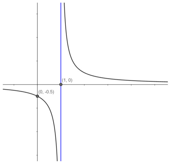
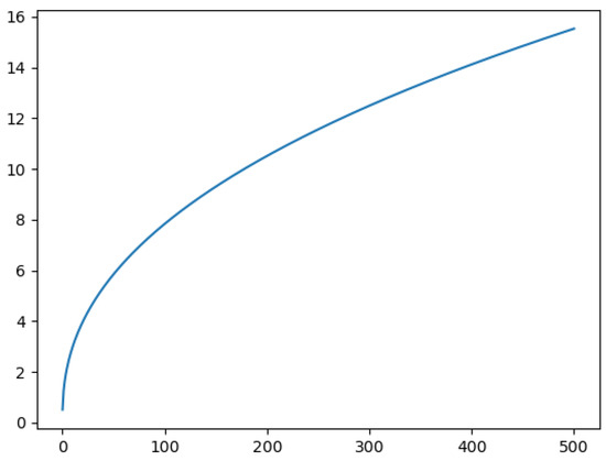
Figure 5. A plot of the function $g\left(r\right)=\frac{1}{2(r-1)}$.

4.4. The Case r > 1

For $r>1$ we get $v\left(0^{+}\right)=arp{\left(0\right)}^{r-1}=0$ and $v\left(p\right)=ar{p}^{r-1}$

$$⟹y\left(v\left(0^{+}\right)\right)=\sqrt{1+0^2}=1,y\left(v\left(p\right)\right)=\sqrt{1+{\left(ar{p}^{r-1}\right)}^2}$$

$$⟹I=\frac{1}{a(r-1){\left(ar\right)}^{\frac{1}{r-1}}}{\int }_1^{\sqrt{1+{\left(ar{p}^{r-1}\right)}^2}}{(y^2-1)}^{g}dy$$

Denote $b=\sqrt{1+{\left(ar{p}^{r-1}\right)}^2}>1$ and $J={\int }_1^b{(y^2-1)}^{g}dy.$ For $g=\frac{1}{2}$ we can find J using trigonometric substitution, but in that case $r=2$ so it does not give us any progress because we have already covered that case. For $g\in \mathbb{N}$ we must have $r\in \{1+\frac{1}{2g}|g\in \mathbb{N}\}=\{1.5,1.25,1\frac{1}{6},1.125,1.1,\dots \}$ in which case we can use the Binomial Theorem to find J. For a general $r\in (1,\infty )$ we can use Theorem 3:

$$⟹J={\int }_1^b{(y^2-1)}^{g}dy={\int }_1^b\left(\sum _{n=0}^{\infty }\left(\genfrac{}{}{0pt}{}{g}{n}\right){(-1)}^n{y}^{2(g-n)}\right)dy=$$

$$=\sum _{n=0}^{\infty }\left(\left(\genfrac{}{}{0pt}{}{g}{n}\right){(-1)}^n{\int }_1^b{y}^{2(g-n)}dy\right)$$

The interchange of the sum and integral signs is justified because we expanded ${(y^2-1)}^g$ into a power series.

$${\int }_1^b{y}^{2(g-n)}=\left\{\begin{array}{cc}ln\left(b\right)\hfill & 2(g-n)=-1\hfill \\ \frac{b^{2(g-n)+1}-1}{2(g-n)+1}\hfill & 2(g-n)\ne -1\hfill \end{array}\right.$$

4.5. The Case 0 < r < 1

For $0<r<1$, the upper bound $y\left(v\right(p\left)\right)$ is the same as for the case of $r>1$. However, since $v=ar{x}^{r-1}$ the lower bound is now:

$$y\left(v\left(0^{+}\right)\right)=\underset{v\to 0^{+}}{lim}\sqrt{1+{\left(ar{v}^{r-1}\right)}^2}=+\infty$$

Referring to Equation (9):

$$I=\frac{1}{a(r-1){\left(ar\right)}^{\frac{1}{r-1}}}{\int }_{\infty }^{\sqrt{1+{\left(ar{p}^{r-1}\right)}^2}}{(y^2-1)}^{g}dy$$

$$⟹J={\int }_{\infty }^b{(y^2-1)}^{g}dy$$

J is an improper integral. We prove that J converges by using the limit comparison test for integrals:

$$\underset{y\to +\infty }{lim}\frac{{(y^2-1)}^g}{{\left(y^2\right)}^g}=1$$

In addition:

$${\int }_{\infty }^b{\left(y^2\right)}^{g}dy=-{\int }_b^{\infty }\frac{1}{y^{-2g}}dy$$

which converges if $-2g>1\iff g<-\frac{1}{2}$ which is true by expression (10). To have $g\in {\mathbb{Z}}^{-}$ we must have $r\in \{1+\frac{1}{2g}|g\in {\mathbb{Z}}^{-}\}=\{0.5,0.75,\frac{5}{6},0.875,0.9,\dots \}$. Then we can write:

$$J={\int }_{\infty }^b{(y^2-1)}^{g}dy={\int }_{\infty }^b\frac{1}{{(y-1)}^{-g}{(y+1)}^{-g}}dy$$

It is possible to continue by using partial fractions decomposition, though we will not cover a general formula for that case. For a general $r\in (0,1)$ we can use Theorem 3 again, as we did in the previous subsection:

$$J=\sum _{n=0}^{\infty }\left(\left(\genfrac{}{}{0pt}{}{g}{n}\right){(-1)}^n{\int }_{\infty }^b{y}^{2(g-n)}dy\right)=\sum _{n=0}^{\infty }\left(\genfrac{}{}{0pt}{}{g}{n}\right){(-1)}^n\frac{b^{2(g-n)+1}}{2(g-n)+1}$$

5. Minimizing Both Area and Length

In Theorem 5, we proved that the curve $y_1\in B$ which minimizes the area is given with the parameter $a=\frac{t}{r{k}^r}$. Denote that expression for a as $a_S(k,t,r)$. In Theorem 6, we proved that there exists a unique curve $y_2\in B$ which minimizes the length and described a method to calculate the parameter a of that curve. Denote that a as $a_L(k,t,r)$. Our question is whether it is possible for $y_1$ and $y_2$ to be identical. The answer is yes, and we explain under which condition it happens. The curves are identical if and only if their parameter a is equal. So we get the equation:

$$a_S(k,t,r)=a_L(k,t,r)\iff a_L=\frac{t}{r{k}^r}\iff t-r{k}^r{a}_L=0$$

We will explore the function $M(k,t,r):=t-r{k}^r{a}_L$. The implicit equation $M(k,t,r)=0$ defines a relation between our starting parameters $k,t,r$.

Theorem 7.

For all $k,r>0$, there exists $t>0$ such that $M(k,t,r)=0$.

A special case is $r=1$, for which to minimize the area we must have $a=\frac{t}{k}$ and to minimize the length we must have $a=\sqrt[3]{\frac{t}{k}}$. If we equate the expressions for a:

$$a=\sqrt[3]{\frac{t}{k}}=\frac{t}{k}⟹\frac{t}{k}=1⟹t=k$$

Before proving Theorem 7, we prove some lemmas first. It turns out that for all fixed $k,r>0$, the function $M\left(t\right)$ possesses the same properties (see Figure 6). Let $k,r>0$ be fixed values, and we can exclude $r=1$ which has already been discussed.

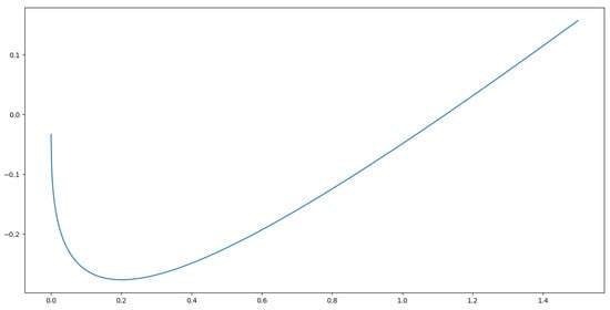
Figure 6. A graph of $M\left(t\right)$ with $k=1$ and $r=2$. $M\left(t\right)$ appears to be continuous, strictly convex, negative at a right neighbourhood of $t=0$, and seems to approach $+\infty$ as $t\to +\infty$.

Lemma 8.

For all $v>0$:

$$a_L\left(t\right)\le \frac{L\left(v\right)-t}{k^r}$$

Proof. 

In the proof of Lemma 4, we saw that $L\left(a\right)\ge t+a{k}^r$. Note that $L\left(v\right)\ge m$, where m is the minimum of L, which is guaranteed to exist by Theorem 6. In addition, $t+a{k}^r\ge L\left(v\right)\iff a\ge \frac{L\left(v\right)-t}{k^r}$. As a result, we can conclude that minimum is attained on the interval $(0,\frac{L\left(v\right)-t}{k^r})$, therefore $a_L\left(t\right)\le \frac{L\left(v\right)-t}{k^r}$. □

Lemma 9.

For all $v>0$:

$$L\left(v\right)\le p\left(v\right)+t+v{k}^r$$

Proof. 

$$\begin{array}{c}L\left(v\right)={\int }_0^{p\left(v\right)}\sqrt{1+{\left(vr{x}^{r-1}\right)}^2}dx\le {\int }_0^{p\left(v\right)}\sqrt{{\left(1+vr{x}^{r-1}\right)}^2}=\hfill \\ \hspace{1em}\hspace{1em}\hspace{1em}\hspace{1em}\hspace{1em}\hspace{1em}\hspace{1em}\hspace{1em}\hspace{1em}\hspace{1em}\hspace{1em}\hspace{1em} ={\left.x+v{x}^r\right|}_0^{p\left(v\right)}=p\left(v\right)+v\left(\frac{t}{v}+k^r\right)=p\left(v\right)+t+v{k}^r\hfill \end{array}$$

□

Lemma 10.

$a_L\left(t\right)\to 0$ as $a\to +\infty$

Proof. 

Using Lemmas 8 and 9, we obtain the following bounds:

$$0\le \frac{a_L\left(t\right)}{t}\le \frac{L\left(v\right)-t}{t{k}^r}\le \frac{p\left(v\right)+v{k}^r}{t{k}^r}=\frac{1}{t{k}^r}{\left(\frac{t}{v}+k^r\right)}^{\frac{1}{r}}+\frac{v}{t}$$

If we pick $v=t^{1-\frac{r}{2}}$ then:

$$\underset{t\to +\infty }{lim}\frac{v}{t}=\underset{t\to +\infty }{lim}\frac{t^{1-\frac{r}{2}}}{t}=\underset{t\to +\infty }{lim}\frac{1}{t^{\frac{r}{2}}}=0$$

and:

$$\underset{t\to +\infty }{lim}\frac{1}{t{k}^r}{\left(\frac{t}{v}+k^r\right)}^{\frac{1}{r}}=\underset{t\to +\infty }{lim}\frac{1}{t{k}^r}{\left(\frac{t}{t^{1-\frac{r}{2}}}+k^r\right)}^{\frac{1}{r}}=0$$

therefore, we found $v>0$ such that:

$$\underset{t\to +\infty }{lim}\frac{p\left(v\right)+v{k}^r}{t{k}^r}=0$$

and by the squeeze theorem we conclude that ${lim}_{t\to +\infty }\frac{a_L\left(t\right)}{t}=0$. □

Lemma 11.

$M\left(t\right)\to +\infty$ as $t\to +\infty$

Proof. 

Using Lemma 10:

$$\underset{t\to +\infty }{lim}M\left(t\right)=\underset{t\to +\infty }{lim}t-r{k}^r{a}_L\left(t\right)=\underset{t\to +\infty }{lim}t\left(1-r{k}^r\frac{a_L\left(t\right)}{t}\right)=+\infty$$

□

Lemma 12.

For all $v>0$:

$$a_L\left(t\right)\ge \frac{t}{{\left(L\left(v\right)\right)}^r-k^r}$$

Proof. 

The lemma can be proved similarly to how we proved Lemma 8, using the fact that $L\left(a\right)\ge {\left(\frac{t+a{k}^r}{a}\right)}^{\frac{1}{r}}$ which we saw in the proof of Lemma 3. □

Lemma 13.

There exists a right neighbourhood of $t=0$ in which $M\left(t\right)<0$.

Proof. 

Using Lemma 12, we can bound $M\left(t\right)$ from above as such:

$$M\left(t\right)=t-r{k}^r{a}_L\left(t\right)\le t-r{k}^r\frac{t}{{\left(L\left(v\right)\right)}^r-k^r}=t\left(\frac{{\left(L\left(v\right)\right)}^r-k^r-r{k}^r}{{\left(L\left(v\right)\right)}^r-k^r}\right).$$

We prove that there exists a right neighbourhood of $t=0$ such that this upper bound is negative. As a consequence, $M\left(t\right)$ will be negative at that same neighbourhood. First, notice that the denominator is always positive since:

$$L\left(v\right)={\int }_0^{p\left(v\right)}\sqrt{1+{\left(vr{x}^{r-1}\right)}^2}dx\ge {\left(\frac{t+v{k}^r}{v}\right)}^{\frac{1}{r}}\Rightarrow {\left(L\left(v\right)\right)}^r-k^r=\frac{t}{v}>0$$

We prove that there exists a right neighbourhood of $t=0$ such that the numerator is negative. We split into two cases:

• Case 1. Assume $r>\frac{1}{2}$, since

  $$p\left(v\right)={\left(\frac{t}{v}+k^r\right)}^{\frac{1}{r}}\ge k,$$

  then

  $$L\left(v\right)={\int }_0^{p\left(v\right)}\sqrt{1+{\left(vr{x}^{r-1}\right)}^2}dx\ge {\int }_0^{p\left(v\right)}dx\ge k$$
  In addition:

  $$\begin{array}{cc}\hfill L\left(v\right)& ={\int }_0^{p\left(v\right)}\sqrt{1+{\left(vr{x}^{r-1}\right)}^2}dx\le {\int }_0^{p\left(v\right)}\left(1+v^2{r}^2{x}^{2r-2}\right)dx\hfill \\ & ={\left.x+\frac{v^2{r}^2}{2r-1}{x}^{2r-1}\right|}_0^{p\left(v\right)}={\left(\frac{t}{v}+k^r\right)}^{\frac{1}{r}}+\frac{v^2{r}^2{\left(\frac{t}{v}+k^r\right)}^{\frac{2r-1}{r}}}{2r-1}.\hfill \end{array}$$
  Note that the substitution at $x=0$ is justified because $r>\frac{1}{2}\Rightarrow 2r-1>0$. If we let $v=\sqrt{t}$, we get:

  $$\underset{t\to 0^{+}}{lim}\left({\left(\frac{t}{v}+k^r\right)}^{\frac{1}{r}}+\frac{v^2{r}^2{\left(\frac{t}{v}+k^r\right)}^{\frac{2r-1}{r}}}{2r-1}\right)=k$$
  Hence, using the squeeze theorem we conclude that ${lim}_{t\to 0^{+}}L\left(v\right)=k$. It follows that ${lim}_{t\to 0^{+}}\left({\left(L\left(v\right)\right)}^r-k^r-r{k}^r\right)=-r{k}^r<0$. The last limit implies that the numerator is negative at some right neighbourhood of $t=0$.
• Case 2. Assume $0<r\le \frac{1}{2}$. Let $v=\sqrt{t}$ again. We prove again that ${lim}_{t\to 0^{+}}L\left(v\right)=k$. We write:

  $$\begin{array}{cc}\hfill L\left(v\right)& =L\left(\sqrt{t}\right)={\int }_0^{{\left(\sqrt{t}+k^r\right)}^{\frac{1}{r}}}\sqrt{1+t{\left(r{x}^{r-1}\right)}^2}dx\hfill \\ \hfill & ={\int }_0^k\sqrt{1+t{\left(r{x}^{r-1}\right)}^2}dx+{\int }_k^{{\left(\sqrt{t}+k^r\right)}^{\frac{1}{r}}}\sqrt{1+t{\left(r{x}^{r-1}\right)}^2}dx\hfill \end{array}$$
  Note that:

  $$\begin{array}{c}\left|{\int }_k^{{\left(\sqrt{t}+k^r\right)}^{\frac{1}{r}}}\sqrt{1+t{\left(r{x}^{r-1}\right)}^2}dx\right|\le \hfill \\ \hspace{1em}\hspace{1em}\hspace{1em}\hspace{1em}\hspace{1em}\hspace{1em}\hspace{1em}\hspace{1em}\hspace{1em}\hspace{1em}\le \left({\left(\sqrt{t}+k^r\right)}^{\frac{1}{r}}-k\right)\sqrt{1+t{r}^2{\left(\sqrt{t}+k^r\right)}^{\frac{2\left(r-1\right)}{r}}}\underset{t\to 0^{+}}{\to }0\hfill \end{array}$$
  For the other integral, we use Theorem 4. Denote

  $$F\left(t\right)={\int }_0^k\sqrt{1+t{\left(r{x}^{r-1}\right)}^2}dx$$

  and $J=[0,1]$. We are indeed dealing with an improper integral here since $0<r\le \frac{1}{2}$. Our integrand is continuous for all $(x,t)\in (0,k]\times [0,1]$. In addition, the improper integral converges uniformly by the Weierstrass M-test, since:

  $$\sqrt{1+t{\left(r{x}^{r-1}\right)}^2}\le \sqrt{1+r^2{x}^{2r-2}}$$

  and ${\int }_0^k\sqrt{1+r^2{x}^{2r-2}}dx$ converges by the limit comparison test with $x^{r-1}$ which converges since $r-1>-1$. As a result, due to Theorem 4, $F\left(t\right)$ is continuous on $[0,1]$, and in particular, ${lim}_{t\to 0^{+}}F\left(t\right)=F\left(0\right)=k\Rightarrow {lim}_{t\to 0^{+}}L\left(v\right)=k$.

□

Lemma 14.

$M\left(t\right)$ is continuous on $(0,\infty )$.

Proof. 

Since $M\left(t\right)=t-r{k}^r{a}_L\left(t\right)$, it is suffice to prove that $a_L\left(t\right)$ is continuous. In Theorem 6, we proved that for all $k,t,r$, the equation $L^{\prime }\left(a\right)=0$ only has one root. $a_L\left(t\right)$ was defined as the single root of the equation $L^{\prime }\left(a\right)=0$. Now, since $k,r$ are constants, but t is not, we can look at the equation $L^{\prime }(a,t)=0$ as an implicit equation. If we denote $Q(a,t)=L^{\prime }(a,t)$ then by Lemma 7, $Q_a^{\prime }\ne 0$. Now, it is also easy to tell, from the proof of Lemma 7, that $Q_a^{\prime }$ is continuous. Similarly, it is straight forward to find an expression for $Q_t^{\prime }$, which proves it is continuous:

$$Q_t^{\prime }=\frac{-p\left(t+ra{k}^r\right)}{{\left(t+a{k}^r\right)}^{2}a{r}^2\sqrt{1+{\left(ar{p}^{\left(r-1\right)}\right)}^2}}$$

Given $t_0\in (0,\infty )$, all of the conditions of the implicit function theorem are satisfied at the point $(a,t)=(a_L\left(t_0\right),t_0)$, which assures us that $a_L\left(t\right)$ is continuous at $t_0$. As a result, $M\left(t\right)$ is continuous for all for all $t\in (0,\infty )$. □

Proof of Theorem 7.

Lemmas 11, 13 and 14 and the intermediate value theorem imply that the equation $M\left(t\right)=0$ has a solution. □

So we already proved the existence of the desired solution which minimizes the area and the length simultaneously. The following theorem provides a sufficient condition for the solution to be unique.

Theorem 8.

Given $k,r>0$, if $a_L(k,t,r)$ is strictly concave as a function of t on $(0,\infty )$, then there is a single $t>0$ such that $M(k,t,r)=0$.

Proof. 

Assume there exist $t_1<t_2$ such that $M\left(t_1\right)=M\left(t_2\right)=0$. $a_L\left(t\right)$ being strictly concave implies that $M\left(t\right)$ is strictly convex. This, along with the fact that $M\left(t_1\right)=M\left(t_2\right)=0$ implies that $M\left(t\right)$ has a global minimum at $t_3\in (t_1,t_2)$ with $M\left(t_3\right)<0$. Lemma 13 implies there exists $t_4<t_1$ such that $M\left(t_4\right)<0$. Then, Lemma 14 together with intermediate value theorem imply there exist $t_5\in (t_4,t_1),t_6\in (t_1,t_3)$ with $M\left(t_5\right)=M\left(t_6\right)$. This again implies that $M\left(t\right)$ has a global minimum on $(t_5,t_6)$, which contradicts the fact that strictly convex functions have at most one global minimum. □

Remark 3.

We have already seen that for $r=1$ we get $a_L\left(t\right)=\sqrt[3]{\frac{t}{k}}$ which is strictly concave as a function of t. In addition, a typical graph of $a_L\left(t\right)$ (see Figure 7) for other values of r also appears to be strictly concave.

Figure 7. A graph of $a_L\left(t\right)$ with $k=1$ and $r=2$, which appears to be strictly concave.

This leads us to the following conjecture.

Conjecture. 

For all $k,r>0$, $a_L(k,t,r)$ is strictly concave as a function of t on $(0,\infty )$.

6. Conclusions and Open Questions

In this manuscript, we proposed a natural optimization problem. Fixing $r>0$, we considered the family of curves of the form $y=-a{x}^r+c$ in the first quadrant passing through a fixed point. We proved that the area minimizer is unique and gave a closed form expression for it and proved the uniqueness of the length minimizer. A result we obtained is that if we tune the height of the fixed point, then we can find a specific height that the two minimizers coincide. We gave a sufficient condition for the uniqueness of that specific height. There remains the open question regarding the concavity of $a_L\left(t\right)$ (we gave a proof for the case $r=1$), or alternatively proving or disproving the uniqueness by a different method. Future work might also consist of exploration of different families of curves or proofs for more general statements about the problem.

References

- Gul, S.; Cohen, R. Efficient Covering of Thin Convex Domains Using Congruent Discs. Mathematics 2021, 9, 3056. [Google Scholar] [CrossRef]
- Freeman, H.; Shapira, R. Determining the Minimum-Area Encasing Rectangle for an Arbitrary Closed Curve. Commun. ACM 1975, 18, 409–413. [Google Scholar] [CrossRef]
- Boscain, U.; Charlot, G.; Rossi, F. Existence of planar curves minimizing length and curvature. Proc. Steklov Inst. Math. 2010, 270, 43–56. [Google Scholar] [CrossRef]
- Sebastian, T.; Klein, P.; Kimia, B. On aligning curves. IEEE Trans. Pattern Anal. Mach. Intell. 2003, 25, 116–125. [Google Scholar] [CrossRef]
- Barequet, G.; Gershon, E.; Kim, M.S. Computing the Minimum Enclosing Circle of a Set of Planar Curves. Comput. Aided Des. Appl. 2005, 2, 301–308. [Google Scholar]
- Albocher, D.; Elber, G. On the computation of the minimal ellipse enclosing a set of planar curves. In Proceedings of the 2009 IEEE International Conference on Shape Modeling and Applications, Beijing, China, 26–28 June 2009; pp. 185–192. [Google Scholar] [CrossRef]
- Schröcker, H.P. Uniqueness results for minimal enclosing ellipsoids. Comput. Aided Geom. Des. 2008, 25, 756–762. [Google Scholar] [CrossRef]
- Bhattacharya, B.; Mukhopadhyay, A. On the Minimum Perimeter Triangle Enclosing a Convex Polygon. In Proceedings of the Discrete and Computational Geometry; Akiyama, J., Kano, M., Eds.; Springer: Berlin/Heidelberg, Germany, 2003; pp. 84–96. [Google Scholar]
- Mitchell, J.S.; Polishchuk, V. Minimum-perimeter enclosures. Inf. Process. Lett. 2008, 107, 120–124. [Google Scholar] [CrossRef]
- Bose, P.; Mora, M.; Seara, C.; Sethia, S. On Computing Enclosing Isosceles Triangles and Related Problems. Int. J. Comput. Geom. Appl. 2011, 21, 25–45. [Google Scholar] [CrossRef]
- Böröczky, K., Jr.; Hernández Cifre, M.A.; Salinas, G. Optimizing area and perimeter of convex sets for fixed circumradius and inradius. Mon. Math. 2003, 138, 95–110. [Google Scholar] [CrossRef]
- Bartle, R.G.; Bartle, R.G. The Elements of Real Analysis; Wiley: New York, NY, USA, 1964; Volume 2. [Google Scholar]
- Trench, W.F. Functions Defined by Improper Integrals, Supplement for Introduction to Real Analysis. 2013. Available online: https://digitalcommons.trinity.edu/mono/7/ (accessed on 1 August 2021).
Publisher’s Note: MDPI stays neutral with regard to jurisdictional claims in published maps and institutional affiliations. |
© 2022 by the authors. Licensee MDPI, Basel, Switzerland. This article is an open access article distributed under the terms and conditions of the Creative Commons Attribution (CC BY) license (https://creativecommons.org/licenses/by/4.0/).