Two-Sample Hypothesis Test for Functional Data

Abstract

In this paper, we develop and study a novel testing procedure that has more a powerful ability to detect mean difference for functional data. In general, it includes two stages: first, splitting the sample into two parts and selecting principle components adaptively based on the first half-sample; then, constructing a test statistic based on another half-sample. An extensive simulation study is presented, which shows that the proposed test works very well in comparison with several other methods in a variety of alternative settings.

1. Introduction

In the recent literature, there has been an increasing interest in functional data analysis, with its extensive application in biometrics, chemometrics, econometrics, and medical research, as well as other fields. Functional data have intrinsically infinite dimensions and thus, classical methods for multivariate observations are not applicable. Therefore, it is necessary to develop special techniques for this type of data. There has intensive methodological and theoretical development in function data analysis; see [1,2,3,4,5] and so on.

In functional data analysis, a functional data set or curve can be modeled as independent realizations of an underlying stochastic process:

$$x_i\left(t\right)=\mu \left(t\right)+{\alpha }_i\left(t\right)+{ϵ}_i\left(t\right),i=1,2,\cdots ,n,$$

(1)

where $\mu \left(t\right)$ is the mean function of the stochastic process, ${\alpha }_i\left(t\right)$ is the ith individual function variation from $\mu \left(t\right)$, and ${ϵ}_i\left(t\right)$ is the ith measurement error process. In general, we assume ${\alpha }_i\left(t\right)$ and ${ϵ}_i\left(t\right)$ are independent, and i.i.d. sample from $\alpha \left(t\right)$ and $ϵ\left(t\right)$, respectively, where, $\alpha \left(t\right)\sim \mathrm{SP}(0,\gamma )$, $ϵ\left(t\right)\sim \mathrm{SP}(0,{\gamma }_{ϵ})$, and SP denotes a stochastic process with mean function $\mu \left(t\right)$ and covariance function $\gamma (s,t)$.

The mean function $\mu \left(t\right)$ reflects the underlying trend and can be used as an important index for population response, such as in drug and biomedical purposes, among other. One important statistical inference other than estimation is related to testing of various hypotheses about the mean function. Therefore, we focus on the problem of testing the equality of mean functions in two random samples independently drawn from two functional random variables. There have been some approaches proposed so far to address this problem. For instance, Ref. [6] proposed an adaptive Neyman test, but in the case when the sampling information is in a “discrete” format. Ref. [7] discussed two methods: multivariate analysis-based and bootstrap-based testing.

However, these methods have only been applied in narrow fields and not available for a global testing result. Refs. [8,9] proposed an $L^2$-norm based statistic to test the equality of mean functions. Ref. [10] proposed and studied a so-called Globalized Pointwise F-test, abbreviated as GPF test. The GPF test is in general comparable with the $L^2$-norm-based test and the F-type test adopted for the one-way ANOVA problem. Then, Ref. [11] proposed the $F_{\max }$-test; via some simulation studies, it was found that in terms of both level accuracy and power, the $F_{\max }$-test outperforms the Globalized Pointwise F (GPF) test of [10] when the functional data are highly or moderately correlated, and its performance is comparable with the latter otherwise. Ref. [5] proposed a statistic based on the functional principal component emi-distances. Furthermore, they gave a normalized version of the functional principal components that has a chi-square limit distribution. The statistic is scale-invariant. However, this method require pre-specifying a threshold to choose the leading principal components (PCs), where PCs are ranked based on eigenvalues. They chose the number of PCs, for example, d, based on the percentage of variance explained for the functional covariates. This method has two drawbacks: one is that it can only detect mean differences in this d-dimensional subspace; the other is that different thresholds often lead to different tests, whose power depends on the particular simple alternative hypothesis.

In this paper, we develop and study a novel testing procedure that overcomes the drawback that many tests can only detect mean difference in the d-dimensional subspace. Furthermore, the novel testing procedure is very powerful in the cases when there are differences in middle part and latter part of two function sequences. Additionally, we derived the asymptotic distribution of the new test statistics under the alternative hypothesis, which is the key difficulty in the current approach. In general, the novel testing procedure includes two stages: first, split the sample into two parts and select PCs adaptively based on the first half-sample; then, construct the test statistic based on another half-sample. Sample splitting is often used in high-dimension regression problems because most computationally efficient selection algorithms cannot guard against inclusion of noise variables. Asymptotically valid p-values are not available. Ref. [12] adopted this technology to reduce the number of variables to a manageable size using the first split sample and apply classical variable selection techniques with the remaining variables, using the data from the second split.

In our procedure, we mainly adopt two methods to select PCs in the first stage: the adaptive Neyman test [6] and the adaptive ordered Neyman test. At the same time, we also consider selecting PCs based on pre-specifying a threshold; however, this threshold is an association–projection index that combines both the variation and the projection along each direction. The purpose of splitting the sample is two-fold: (1) to decrease the random noise effect in the first stage; (2) to derive the asymptotic distribution of the test statistic. From simulation results, we can see that our testing procedure asymptotically achieves the pre-specified significance level, and enjoys certain optimality in terms of its power, even when the population is a non-Gaussian process.

This paper is organized as follows. In Section 2, we introduce the test problem and briefly review the existing global two-sample test methods. Section 3 proposes our testing procedure. Simulation studies are given in Section 4. A real-data example is analyzed in Section 5. Section 6 concludes the present work. The derivations are given in Appendix A.

2. The Testing Problem for Functional Data

2.1. Preliminary

Let $\mathrm{SP}$($\mu ,\Gamma$) denote a stochastic process with mean function $\mu \left(t\right),t\in T$ and covariance function $\Gamma (s,t),s,t\in T$, where $T\in [0,1]$. Suppose we have the following two independent function samples:

$$X_1\left(t\right),\cdots ,X_{n_1}\left(t\right)\sim \mathrm{SP}({\mu }_1,{\Gamma }_1(s,t)),$$

(2)

$$Y_1\left(t\right),\cdots ,Y_{n_2}\left(t\right)\sim \mathrm{SP}({\mu }_2,{\Gamma }_2(s,t)),$$

(3)

where ${\Gamma }_1(s,t)$ denotes the covariance function of the function data $X\left(t\right)$ and ${\Gamma }_2(s,t)$ denotes the covariance function of the function data $Y\left(t\right)$. However, we do not know if ${\Gamma }_1(s,t)$ and ${\Gamma }_2(s,t)$ are equal. We want to test whether the two mean functions are equal:

$$H_0:{\mu }_1\left(t\right)={\mu }_2\left(t\right)\mathrm{vs}.{\mathit{H}}_1:{\mu }_1\left(t\right)\ne {\mu }_2\left(t\right).$$

(4)

Let $\overline{X}\left(t\right),\overline{Y}\left(t\right)$ denote the sample mean functions of the two samples, respectively. First, we have

$${\widehat{\mu }}_1\left(t\right)=\overline{X}\left(t\right),{\widehat{\mu }}_2\left(t\right)=\overline{Y}\left(t\right),$$

(5)

and

$$\sqrt{n}({\widehat{\mu }}_1\left(t\right)-{\widehat{\mu }}_2\left(t\right))\sim \mathrm{SP}\left(\sqrt{n}({\mu }_1\left(t\right)-{\mu }_2\left(t\right)),{\Gamma }_{12}(s,t)\right),$$

(6)

where ${\Gamma }_{12}(s,t)=\frac{{\Gamma }_1(s,t)}{n_1/n}+\frac{{\Gamma }_2(s,t)}{n_2/n},n=n_1+n_2$. ${\Gamma }_{12}(s,t)$ can be written as ${\Gamma }_{12}(s,t)={\displaystyle \sum _{k=1}^{\infty }}{\lambda }_k{\phi }_k\left(s\right){\phi }_k\left(t\right)$, where ${\lambda }_1\ge {\lambda }_2\cdots \ge 0$ are the eigenvalues and ${\phi }_k\left(t\right),k=1,\cdots ,\infty$ are eigenfunctions satisfying ${\int }_T{\phi }_k{\left(t\right)}^{2}dt=1$ and ${\int }_T{\phi }_k\left(t\right){\phi }_l\left(t\right)dt=0,k\ne l$.

It is easy to see that ${\widehat{\Gamma }}_1(s,t)=\frac{1}{n_1}{\displaystyle \sum _{i=1}^{n_1}}(X_i\left(t\right)-{\widehat{\mu }}_1\left(t\right))(X_i\left(s\right)-{\widehat{\mu }}_1\left(s\right))$, ${\widehat{\Gamma }}_2(s,t)=\frac{1}{n_2}{\displaystyle \sum _{i=1}^{n_2}}$$(Y_i\left(t\right)-{\widehat{\mu }}_2\left(t\right))(Y_i\left(s\right)-{\widehat{\mu }}_2\left(s\right))$ and ${\widehat{\Gamma }}_{12}(s,t)=\frac{{\widehat{\Gamma }}_1(s,t)}{n_1/n}+\frac{{\widehat{\Gamma }}_2(s,t)}{n_2/n}$.

${\widehat{\Gamma }}_{12}(s,t)$ can also be written in as an eigen-decomposition

$${\widehat{\Gamma }}_{12}(s,t)={\displaystyle \sum _{k=1}^{\infty }}{\widehat{\lambda }}_k{\widehat{\phi }}_k\left(s\right){\widehat{\phi }}_k\left(t\right),$$

(7)

where the nonincreasing sequence $({\widehat{\lambda }}_k:k\ge 1)$ is the sample eigenvalues and $({\widehat{\phi }}_k:k\ge 1)$ are the corresponding eigenfunctions forming an orthonormal basis of $L_2[0,1]$.

To simplify notation, we use the symbol $\Gamma$ for both the kernel and the operator. Now, the functional Mahalanobis semi-distance between ${\widehat{\mu }}_1\left(t\right)$ and ${\widehat{\mu }}_2\left(t\right)$ is defined as:

$$d_{FM}^2({\widehat{\mu }}_1,{\widehat{\mu }}_2)=⟨{\widehat{\Gamma }}_{12,p_n}^{-\frac{1}{2}}\sqrt{n}({\widehat{\mu }}_1-{\widehat{\mu }}_2),{\widehat{\Gamma }}_{12,p_n}^{-\frac{1}{2}}\sqrt{n}({\widehat{\mu }}_1-{\widehat{\mu }}_2)⟩.$$

(8)

Plugging (6) into (7), we have

$$d_{FM}^2({\widehat{\mu }}_1,{\widehat{\mu }}_2)={\displaystyle \sum _{k=1}^{p_n}}\frac{n{⟨{\widehat{\mu }}_1-{\widehat{\mu }}_2,{\widehat{\phi }}_k⟩}^2}{{\widehat{\lambda }}_k}.$$

(9)

2.2. Existing Global Testing Methods

Although there is significant literature discussing the equality of means for two functional data sets, they can be roughly grouped into a few broad categories, as follows.

(1)

$L_2$-norm-based test

The test is based on the $L_2$-norm of the difference between ${\widehat{\mu }}_1\left(t\right)$ and ${\widehat{\mu }}_2\left(t\right)$:

$$T_L=n{\parallel {\widehat{\mu }}_1\left(t\right)-{\widehat{\mu }}_2\left(t\right)\parallel }^2=n\int {({\widehat{\mu }}_1\left(t\right)-{\widehat{\mu }}_2\left(t\right))}^{2}dt.$$

(10)

Ref. [8] proved that $T_L=n\int {({\widehat{\mu }}_1\left(t\right)-{\widehat{\mu }}_2\left(t\right))}^{2}dt\stackrel{d}{=}{\displaystyle \sum _{k=1}^{\infty }}{\lambda }_k{A}_k+o_p\left(1\right)$, $A_k\sim {\chi }_1^2\left(\frac{n{u}_k^2}{{\lambda }_k}\right)$, where $X\stackrel{d}{=}Y$ denotes that X and Y have the same distribution, and $u_k={\int }_0^1({\mu }_1\left(t\right)-{\mu }_2\left(t\right)){\phi }_k\left(t\right)dt,k=1,2,\cdots .$ Furthermore, they use the two-cumulant matched ${\chi }^2$ approximation method and obtained an approximate distribution of $T_L$, which is, $\alpha {\chi }_d^2+\beta$, where

$$\alpha =\frac{{\displaystyle \sum _{k=1}^{\infty }}{\widehat{\lambda }}_k^3}{{\displaystyle \sum _{k=1}^{\infty }}{\widehat{\lambda }}_k^2},d=\frac{{\left\{{\displaystyle \sum _{k=1}^{\infty }}{\widehat{\lambda }}_k^2\right\}}^3}{{\left\{{\displaystyle \sum _{k=1}^{\infty }}{\widehat{\lambda }}_k^3\right\}}^2},\beta ={\displaystyle \sum _{k=1}^{\infty }}{\widehat{\lambda }}_k-\frac{{\left\{{\displaystyle \sum _{k=1}^{\infty }}{\widehat{\lambda }}_k^2\right\}}^2}{{\displaystyle \sum _{k=1}^{\infty }}{\widehat{\lambda }}_k^3}.$$

Then, they have $P(T_L>K)\approx P({\chi }_d^2>(K-\beta )/\alpha ).$

(2)

Projection-based Test

Ref. [5] considered projecting the observed mean difference onto the space spanned by ${\widehat{\phi }}_1,\cdots ,{\widehat{\phi }}_d$, where d is determined based on the percentage of eigenvalues, constructed the following test statistic:

$$T_H={\displaystyle \sum _{k=1}^d}{⟨\sqrt{n}({\widehat{\mu }}_1-{\widehat{\mu }}_2),{\widehat{\phi }}_k⟩}^2.$$

(11)

Given d, the asymptotic distribution of $T_H$ under the null hypothesis is the distribution of ${\displaystyle \sum _{k=1}^d}{\lambda }_k{Z}_k^2$, where $Z_k,k=1,\cdots ,d$ are independent standard normal random variables. Alternately, they proposed a normalized version of $T_H$ which is given by

$$N{T}_H={\displaystyle \sum _{k=1}^d}{⟨\sqrt{n}({\widehat{\mu }}_1-{\widehat{\mu }}_2),{\widehat{\phi }}_k⟩}^2/{\widehat{\lambda }}_k,$$

(12)

Then, under the null hypothesis, $N{T}_H$ has an asymptotic ${\chi }_d^2$ distribution.

(3)

F-test

Finally, we describe the testing procedure proposed by [13]. Although they proposed a functional F test in a functional linear regression setting, the method can be specified for our two sample test as follows.

The F-test statistic for our setting is

$$T_F=\frac{RS{S}_0-RS{S}_1}{RS{S}_1/(n-1)},$$

(13)

where

$$\begin{array}{ccc}\hfill RS{S}_1& =& {\displaystyle \sum _{i=1}^{n_1}}{\int }_0^1{(X_i\left(t\right)-\overline{X}\left(t\right))}^{2}dt+{\displaystyle \sum _{i=1}^{n_2}}{\int }_0^1{(Y_i\left(t\right)-\overline{Y}\left(t\right))}^{2}dt,\hfill \\ \hfill RS{S}_0& =& {\displaystyle \sum _{i=1}^{n_1}}{\int }_0^1{(X_i\left(t\right)-\overline{Z}\left(t\right))}^{2}dt+{\displaystyle \sum _{i=1}^{n_2}}{\int }_0^1{(Y_i\left(t\right)-\overline{Z}\left(t\right))}^{2}dt,\hfill \\ \hfill \overline{Z}\left(t\right)& =& \frac{n_1\overline{X}\left(t\right)+n_2\overline{Y}\left(t\right)}{n_1+n_2}.\hfill \end{array}$$

Ref. [13] also presented the distribution of the F-test as $\frac{{\displaystyle \sum _{k=1}^{\infty }}{\lambda }_k{\chi }_1^2}{{\displaystyle \sum _{k=1}^{\infty }}{\lambda }_k{\chi }_{n-2}^2}.$ In practice, they also applied the idea of [14] approximation to derive approximate distribution of F-statistic, that is, $({\chi }_{f_1}^2/f_1)/({\chi }_{f_2}^2/f_2)$, which is an ordinary F distribution with degrees of freedom $f_1$ and $f_2$, where $f_1={\left({\displaystyle \sum _{k=1}^{\infty }}{\widehat{\lambda }}_k\right)}^2/{\displaystyle \sum _{k=1}^{\infty }}{\widehat{\lambda }}_k^2$, $f_2=(n-2){\left({\displaystyle \sum _{k=1}^{\infty }}{\widehat{\lambda }}_k\right)}^2/{\displaystyle \sum _{k=1}^{\infty }}{\widehat{\lambda }}_k^2$.

3. Our Testing Procedure

In order to determine the number of PCs $p_n$ adaptively and find significant parts to construct a more powerful test statistic, we propose a two-stage procedure via a data-splitting technique. With the help of this technique, we can derive the distribution of the test statistic.

First, we assume that the sample size is even for simplicity and randomly split samples into two groups: $(X^{\left(1\right)},Y^{\left(1\right)})$ and $(X^{\left(2\right)},Y^{\left(2\right)})$. In the first stage, we choose $p_n$ based on the adaptively truncated Hotelling $T^2$ order statistic via the first group sample $(X^{\left(1\right)},Y^{\left(1\right)})$. In the second stage, we construct the test statistic via the second group sample $(X^{\left(2\right)},Y^{\left(2\right)})$ and $p_n$.

Next, we show three methods of choosing $p_n$ in a general case.

Denote ${\widehat{V}}_k^{\left(1\right)}={⟨\sqrt{n/2}({\widehat{\mu }}_1^{\left(1\right)}-{\widehat{\mu }}_2^{\left(1\right)}),{\widehat{\phi }}_k^{\left(1\right)}⟩}^2/{\widehat{\lambda }}_k^{\left(1\right)},k=1,\cdots ,d,\cdots .$ In practice, since many of the trailing eigenvalues are close to zero and ${\widehat{V}}_k$ will be very large for a large k. Hence, we generally give the cutoff $d_n$ a high threshold, for example, $d_n=max\{k:{\widehat{\lambda }}_k/{\displaystyle \sum _{t=1}^k}{\widehat{\lambda }}_t>0.001\}$. For most inference problems, there is no optimal test, but the adaptive Neyman tests have been shown to work well against a broad range of alternatives. Therefore, we choose $p_n$ adaptively based on the following adaptive Neyman test methods. One method is maximizing normalized (8) (in the Appendix A we have proven ${\widehat{V}}_k$ has an approximate ${\chi }_1^2$ distribution), that is,

$$p_{1n}={\mathrm{argmax}}_{1\le d\le d_n}\frac{{\displaystyle \sum _{k=1}^d}{\widehat{V}}_k^{\left(1\right)}-d}{\sqrt{2d}}.$$

Considering some possible nonsignificant ${\widehat{V}}_k^{\left(1\right)}$ terms, we propose another method that maximizes the sun of normalized order statistic $V_{\left(k\right)}$, that is,

$$p_{2n}={\mathrm{argmax}}_{1\le d\le d_n}\frac{{\displaystyle \sum _{k=1}^d}{\widehat{V}}_{\left(k\right)}^{\left(1\right)}-E\left({\displaystyle \sum _{k=1}^d}{\widehat{V}}_{\left(k\right)}^{\left(1\right)}\right)}{\sqrt{\mathrm{var}\left({\displaystyle \sum _{k=1}^d}{\widehat{V}}_{\left(k\right)}^{\left(1\right)}\right)}},$$

where ${\widehat{V}}_{\left(k\right)}^{\left(1\right)}$ is the k-th order statistic of ${\widehat{V}}_k^{\left(1\right)},k=1,\cdots ,d$ in decreasing order. Unfortunately, there is no closed form since it involves order statistics. However, empirical approximations of this maximum value can be conducted by very fast Monte Carlo approximations. The third method is a hard threshold truncation method, but we truncate at the d-th term based on the percentage of ${\widehat{V}}_k$, which combines both the variation and the projection along each direction. In our simulation, we set a truncation threshold as [5] projection-based test for comparison.

Remark 1.

$p_{1n}$ and $p_{2n}$ are chosen adaptively based on the first group data. For the convenience of follow-up theoretical analysis, we denote them as $p_n$ uniformly.

After we derive $p_n$ in the first stage, we construct the following statistic based on the second group sample as follows:

$$T_{1A}={\displaystyle \sum _{k=1}^{p_n}}{\widehat{V}}_k^{\left(2\right)},$$

$$T_{2A}={\displaystyle \sum _{k=1}^{p_n}}{\widehat{V}}_{\left(k\right)}^{\left(2\right)},$$

$$N{T}_{1A}=\frac{{\displaystyle \sum _{k=1}^{p_n}}{\widehat{V}}_k^{\left(2\right)}-p_n}{\sqrt{2p_n}},$$

$$N{T}_{2A}=\frac{{\displaystyle \sum _{k=1}^{p_n}}{\widehat{V}}_{\left(k\right)}^{\left(2\right)}-E\left({\displaystyle \sum _{k=1}^{p_n}}{\widehat{V}}_{\left(k\right)}^2\right)}{\sqrt{\mathrm{var}\left({\displaystyle \sum _{k=1}^{p_n}}{\widehat{V}}_{\left(k\right)}^2\right)}},$$

where

$${\widehat{V}}_k^{\left(2\right)}={⟨\sqrt{n/2}({\widehat{\mu }}_1^{\left(2\right)}-{\widehat{\mu }}_2^{\left(2\right)}),{\widehat{\phi }}_k^{\left(2\right)}⟩}^2/{\widehat{\lambda }}_k^{\left(2\right)}$$

To derive the asymptotic distribution of $T_{1A}$, $T_{2A}$, $N{T}_{1A}$, and $N{T}_{2A}$, we make the following assumptions:

Assumption 1.

There exist constants $a>1$ and C such that ${\lambda }_k-{\lambda }_{k+1}\ge C{k}^{-a-1}$ for $k\ge 1$ and $C^{-1}{k}^{-a}\le {\lambda }_k\le C{k}^{-a}.$

Assumption 2.

${\int }_{l}E{X}^4<\infty ,{\int }_{l}E{Y}^4<\infty .$

Assumption 3.

$\tau =\underset{n\to \infty }{lim}\frac{n_1}{n},0<\tau <1.$

Assumption 4.

$p_n^{2a+3}{m}^{-1}=o_p\left(1\right)$, where $m=min(n_1,n_2).$

Assumptions 1 and 2 are regular in functional principle component analysis (FPCA). Assumption 1 implies that ${\lambda }_k\ge C{k}^{-a}$. Because the covariance functions are bounded, one has $a>1$. Assumption 1 essentially assumes that all the eigenvalues are positive, but decay exponentially. Assumption 3 requires that the two sample sizes $n_1,n_2$ tend to ∞ proportionally. Assumption 4 specifies the growing rate of $p_n$. In related literature e.g., [15], to guarantee estimation consistency, $p_n$ is usually assumed to satisfy $p_n^{a+1}{n}^{-1}=o_p\left(1\right)$.

Theorem 1.

Under $H_0$, $\sqrt{n}(\overline{X}-\overline{Y})\stackrel{d}{⟶}G$, where G is a Gaussian process with mean zero and covariance function Γ, where $\Gamma (s,t)=\frac{{\Gamma }_1(s,t)}{\tau }+\frac{{\Gamma }_2(s,t)}{1-\tau }.$

The proof of Theorem 1 follows the trivial central limit of the stochastic process and we omit it.

Remark 2.

We can write G as $G={\displaystyle \sum _{j=1}^{\infty }}{\eta }_j\sqrt{{\lambda }_j}{\phi }_j$, where ${\eta }_j,j\ge 1$ are i.i.d centered real Gaussian random variables with variance 1.

Theorem 2.

Under Assumptions 1–4, there exist some increasing sequences ${\left(p_n\right)}_n$ such that under $H_0$

$$\underset{p_n\to \infty }{lim}P(N{T}_{1A}\le x)=\Phi \left(x\right),$$

(14)

where $\Phi \left(x\right)$ denotes the cumulative distribution function (cdf) of standard normal distribution.

Theorem 3.

Under Assumptions 1–4, the test statistic $T_{2A}$ is approximately equivalent to ${\displaystyle \sum _{k=1}^{p_n}}{\chi }_{\left(k\right)}^2$ (1) under $H_0$, where ${\chi }_{\left(1\right)}^2\left(1\right),\cdots ,{\chi }_{\left(p_n\right)}^2\left(1\right)$ are order statistics (in a decreasing order) of $p_n$${\chi }^2\left(1\right)$ random variables.

Remark 3.

The asymptotic null distribution of $T_{2A}$ is affected not only by the values of ${\widehat{V}}_k^{\left(2\right)}$, but also by the order of them. In practice, empirical approximations of quantiles and tail probability of the null distribution of $T_{2A}$ can be deduced by very fast Monte Carlo approximations.

Theorem 4.

Under Assumptions 1–4 and $H_0$,

$$\underset{(m,p_n)\to \infty }{lim}P(N{T}_{2A}\le x)=\Phi \left(x\right),$$

(15)

where $\Phi \left(x\right)$ denotes the cdf of the standard normal distribution.

To obtain the asymptotic distribution of $N{T}_{1A}$ under the alternative in (3), we choose the local alternative, as defined in the following assumption:

Assumption 5.

$$H_{1n}:{\mu }_1\left(t\right)-{\mu }_2\left(t\right)=n^{-\frac{1}{2}}u\left(t\right),$$

(16)

where $u\left(t\right)$ is any fixed real function such that $0<\Vert u\Vert <\infty .$

Then, we have the following asymptotic power of $N{T}_{1A}$:

Theorem 5.

Under Assumptions 1–6, the asymptotic distribution of the $N{T}_{1A}$ is given by

$$\underset{(m,p_n)\to \infty }{lim}P(N{T}_{1A}>z_{1-\alpha })=\Phi (-z_{1-\alpha }+\parallel {\Gamma }_{12}^{-1}u\left(t\right){\parallel }^2),$$

where P denotes that the distribution have been obtained under the alternative, and $z_{1-\alpha }$ is the upper $(1-\alpha )100\%$ point of the standard normal distribution.

Theorem 6.

Under Assumptions 1–5, the distribution of the $T_{2A}$ is approximately equivalent to a noncentral ${\chi }^2$ distribution ${\chi }_{p_n}^{2*}\left({\zeta }_0\right)$, where

$${\zeta }_0={\displaystyle \sum _{k=1}^{p_n}}{V}_{\left(k\right)}^2,$$

and $V_k^2=\frac{{⟨\sqrt{n/2}({\mu }_1-{\mu }_2),{\phi }_k^{\left(2\right)}⟩}^2}{{\lambda }_k^{\left(2\right)}}=\frac{{⟨u\left(t\right),{\phi }_k^{\left(2\right)}⟩}^2}{{\lambda }_k^{\left(2\right)}}.$

4. Simulations

In this section, we report some Monte Carlo simulation results to compare the finite samples performance of the classical and proposed methods on the two sample mean testing problem under different settings, including a fixed simple alternative and sparse signals with varying locations.

4.1. Fixed Simple Alternative

In this subsection, we first look at a simple setting where the alternatives are fixed. We generate curves from two populations that are generated by 40 Fourier bases as

$$X\left(t\right)={\displaystyle \sum _{k=1}^{40}}({\theta }_k^{1/2}{z}_{1k}+{\mu }_{1k}){\varphi }_k\left(t\right),Y\left(t\right)={\displaystyle \sum _{k=1}^{40}}({\theta }_k^{1/2}{z}_{2k}+{\mu }_{2k}){\varphi }_k\left(t\right).$$

Here, $z_{1k},z_{2k}$ are independent standard normal random variables. In each case, we take ${\varphi }_k\left(t\right)=\sqrt{2}\sin \left((k-0.5)\pi t\right),t\in [0,1]$ for $k=1,2,\cdots$ and generate the data on a discrete grid of 100 equispaced points in [0, 1]. We took ${\theta }_k=1/{\left(\pi (k-0.5)\right)}^2$. We choose ${\mu }_{1k}s$ and ${\mu }_{2k}s$ depending on the property that we want to illustrate (see below). We compare power and size under three different methods: Ref. [8] $L_2$-norm based test ($T_L$); Ref. [13]’s F-test $T_F$; Ref. [5]’s projection-based test ($T_H$) with fixed truncation and our two methods. We choose the commonly used threshold $99\%$ to determine the truncated term in [5]’s projection-based test ($T_H$). The results are based on 1000 Monte Carlo replications. In all scenarios, we set the nominal size $\alpha =0.05$.

To cover as many different scenes as possible, we set five different settings referring to the mean difference: (1) the mean differences arise early in the sequence ${\mu }_{1k}s$ and ${\mu }_{2k}s$, that is, $({\mu }_{11},{\mu }_{12},{\mu }_{13},{\mu }_{14},{\mu }_{15},{\mu }_{16})=(0.5,-0.5,1.5,-0.5,1.5,-0.5)$ and ${\mu }_{1k}=0$ for $k>6$, ${\mu }_{2k}={\mu }_{1k}+\delta$ for $k\le 6$, ${\mu }_{2k}=0$ for $k>6$; (2) the mean differences arise in the middle of the sequence ${\mu }_{1k}s$ and ${\mu }_{2k}s$, that is, $({\mu }_{1,11},{\mu }_{1,12},{\mu }_{1,13},{\mu }_{1,14},{\mu }_{1,15},{\mu }_{1,16})=(0.5,-0.5,1.5,-0.5,1.5,-0.5)$ and ${\mu }_{1k}=0$ for other k, ${\mu }_{2k}={\mu }_{1k}+\delta$ for $11\le k\le 16$, ${\mu }_{2k}=0$ for other k; (3) the mean differences arise in the latter part of the sequence ${\mu }_{1k}s$ and ${\mu }_{2k}s$, that is, $({\mu }_{1,21},{\mu }_{1,22},{\mu }_{1,23},{\mu }_{1,24},{\mu }_{1,25},{\mu }_{1,26})=(0.5,-0.5,1.5,-0.5,1.5,-0.5)$ and ${\mu }_{1k}=0$ for other k, ${\mu }_{2k}={\mu }_{1k}+\delta$ for $21\le k\le 26$, ${\mu }_{2k}=0$ for other k; (4) the mean differences are scattered in the first, middle and latter part, that is, $({\mu }_{1,11},{\mu }_{1,12},{\mu }_{1,13},{\mu }_{1,21},{\mu }_{1,22},{\mu }_{1,23})=(0.5,-0.5,1.5,-0.5,1.5,-0.5)$ and ${\mu }_{1k}=0$ for other k, ${\mu }_{2k}={\mu }_{1k}+\delta$ for $k\in \{1,2,11,12,21,22\}$, ${\mu }_{2k}=0$ for other k; (5) the tiny differences appear in all the principal components. In this case, we set ${\mu }_{1k}$ as independent $N(0,1)$ random variables, and ${\mu }_{2k}={\mu }_{1k}+\delta ,1\le k\le 40$.

From Table 1, Table 2, Table 3, Table 4 and Table 5, we can see that these are obvious different performances in different settings. From Table 1, we can see that when the mean difference lies in early part in the sequence, Ref. [5]’s projection-based test ($T_H$) has most powerful performance. This should not be surprising, because their method just chooses projection space spanned by the first few eigenfunctions, where the mean difference lies. From Table 2 we observe that when mean difference lies in the middle part in the sequence, our method has very high power compared to $T_H$, $T_F$ and $T_L$. Particularly, we notice that Ref. [5]’s projection-based test ($T_H$) has a dramatic power loss. From Table 3, we can see that when the mean difference lies in the latter part of the sequence, our method still has the best performance. At the same time, we can find that $T_F$ and $T_L$ have higher power then $T_H$ in this case. This illustrates that $T_F$ and $T_L$ are sensitive to divergence degree and $T_H$ is more sensitive to location of mean difference. Furthermore, we notice that the power of $T_L$ and $T_F$ outperform our method only on large sample sizes and large discrepancies between the null hypothesis and alternative hypothesis. This is understandable, because our method also depends on mean difference projection on space spanned by the eigenfunction, excluding last few eigenfunctions. Table 4 and Table 5 illustrate more general cases. Table 4 demonstrates that when there are tiny differences in all directions, our method is still the most powerful, while $T_L$ and $T_F$ are useless. Table 5 demonstrates the performance of each method when there are differences in the early part, middle part, and latter part. From the simulation results, we can see that in this general case, our method has the most satisfactory performance.

Table 1. Size and power of five methods in Setting 1 (mean difference lies in early part ${\mu }_2[1:6]={\mu }_1[1:6]+\delta$).

${\mathit{n}}_2={\mathit{n}}_1$	$\mathit{\delta }$	${\mathit{T}}_{\mathit{L}}$	${\mathit{T}}_{\mathit{F}}$	${\mathit{T}}_{\mathit{H}}$	${\mathit{NT}}_{1\mathit{A}}$	${\mathit{NT}}_{2\mathit{A}}$
$n_1=120$	0.00	0.067	0.065	0.068	0.045	0.055
	0.10	0.151	0.105	0.461	0.357	0.365
	0.20	0.245	0.258	0.786	0.483	0.471
	0.30	0.405	0.413	0.998	0.872	0.805
$n_1=220$	0.00	0.045	0.053	0.066	0.051	0.065
	0.10	0.265	0.253	0.643	0.482	0.471
	0.20	0.385	0.393	0.881	0.564	0.585
	0.30	0.553	0.512	0.999	0.976	0.918

Table 2. Size and power of five methods in Setting 2 (mean difference lies in middle part ${\mu }_2[11:16]={\mu }_1[11:16]+\delta$).

${\mathit{n}}_2={\mathit{n}}_1$	$\mathit{\delta }$	${\mathit{T}}_{\mathit{L}}$	${\mathit{T}}_{\mathit{F}}$	${\mathit{T}}_{\mathit{H}}$	${\mathit{NT}}_{1\mathit{A}}$	${\mathit{NT}}_{2\mathit{A}}$
$n_1=120$	0.00	0.052	0.063	0.055	0.067	0.066
	0.10	0.352	0.355	0.384	0.876	0.923
	0.20	0.445	0.466	0.448	0.998	0.999
	0.30	0.581	0.592	0.544	0.999	0.999
$n_1=220$	0.00	0.034	0.045	0.066	0.068	0.063
	0.10	0.442	0.461	0.583	0.975	0.923
	0.20	0.565	0.543	0.654	0.999	0.999
	0.30	0.675	0.691	0.685	0.999	0.999

Table 3. Size and power of five methods in Setting 3 (mean difference lies in latter part ${\mu }_2[21:26]={\mu }_1[21:26]+\delta$).

${\mathit{n}}_2={\mathit{n}}_1$	$\mathit{\delta }$	${\mathit{T}}_{\mathit{L}}$	${\mathit{T}}_{\mathit{F}}$	${\mathit{T}}_{\mathit{H}}$	${\mathit{NT}}_{1\mathit{A}}$	${\mathit{NT}}_{2\mathit{A}}$
$n_1=120$	0.00	0.035	0.052	0.054	0.055	0.042
	0.10	0.342	0.355	0.372	0.486	0.497
	0.20	0.565	0.552	0.593	0.744	0.795
	0.30	0.725	0.753	0.765	0.996	0.985
$n_1=220$	0.00	0.065	0.061	0.045	0.052	0.055
	0.10	0.431	0.425	0.456	0.527	0.588
	0.20	0.628	0.635	0.681	0.823	0.885
	0.30	0.864	0.875	0.824	0.999	0.999

Table 4. Size and power of five methods in Setting 4 (mean difference lies in separable part ${\mu }_2[1:2]={\mu }_1[1:2]+\delta$, ${\mu }_2[11:12]={\mu }_1[11:12]+\delta$, ${\mu }_2[21:22]={\mu }_1[21:22]+\delta$).

${\mathit{n}}_2={\mathit{n}}_1$	$\mathit{\delta }$	${\mathit{T}}_{\mathit{L}}$	${\mathit{T}}_{\mathit{F}}$	${\mathit{T}}_{\mathit{H}}$	${\mathit{NT}}_{1\mathit{A}}$	${\mathit{NT}}_{2\mathit{A}}$
$n_1=120$	0.00	0.045	0.053	0.067	0.068	0.062
	0.10	0.162	0.165	0.326	0.463	0.554
	0.20	0.205	0.272	0.466	0.963	0.955
	0.30	0.361	0.32	0.565	0.999	0.999
$n_1=220$	0.00	0.045	0.038	0.067	0.045	0.068
	0.10	0.192	0.215	0.393	0.497	0.605
	0.20	0.282	0.314	0.516	0.999	0.999
	0.30	0.461	0.465	0.689	1.000	1.000

Table 5. Size and power of five methods in Setting 5 (difference averaged in total vector ${\mu }_2={\mu }_1+\delta {\mathbf{1}}_{40}$).

${\mathit{n}}_2={\mathit{n}}_1$	$\mathit{\delta }$	${\mathit{T}}_{\mathit{L}}$	${\mathit{T}}_{\mathit{F}}$	${\mathit{T}}_{\mathit{H}}$	${\mathit{NT}}_{1\mathit{A}}$	${\mathit{NT}}_{2\mathit{A}}$
$n_1=120$	0.00	0.045	0.052	0.068	0.065	0.053
	0.10	0.182	0.179	0.366	0.794	0.836
	0.20	0.372	0.364	0.854	0.999	0.999
	0.30	0.577	0.564	0.896	1.000	1.000
$n_1=220$	0.00	0.036	0.045	0.062	0.063	0.065
	0.10	0.212	0.249	0.905	0.826	0.887
	0.20	0.413	0.424	0.935	0.999	0.999
	0.30	0.625	0.636	0.943	1.000	1.000

We also conducted simulation studies under other similar scenarios. As they demonstrated similar patterns to those discussed above, we omit them here to save space.

It is worth noting that the proposed method has a first stage with randomly split data. There could be a potential limitation with large randomness. In order to understand the robustness for this splitting, we perform some supporting simulation studies, again considering multi-fold cross validation (CV), including two-fold CV, five-fold CV, and ten-fold CV. For convenience, we use the same data setting of Table 5. The results are shown in Table 6. From Table 6, we can see that in most cases, the hypothesis is robust for this splitting.

Table 6. Size and power of $N{T}_{2A}$ in Setting 5 (difference averaged in total vector ${\mu }_2={\mu }_1+\delta {\mathbf{1}}_{40}$).

$\mathit{\delta }$
${\mathit{n}}_{\mathbf{2}}={\mathit{n}}_{\mathbf{1}}=\mathbf{120}$	0.00	0.1	0.2	0.3
two-fold CV	0.058	0.468	0.786	0.947
five-fold CV	0.056	0.459	0.772	0.943
ten-fold CV	0.053	0.465	0.765	0.978

4.2. Sparse Signals with Varying Locations

In this section, we demonstrate the performance of different tests under signals with varying locations. We set ${\mu }_{1k}(1\le k\le 40)$ as independent $U(0,1)$ random variables, and ${\mu }_{2k}={\mu }_{1k}+\delta$, where k is six random locations out of 40. In Setting 1, the signal of difference appears randomly in six of the first twenty principal components; we denote $M(20,6)$. In Setting 2, the signal of difference appears in six of forty principal components; we denote $M(40,6)$. The simulation results are illustrated in Table 7 and Table 8. From the simulation results, we can see that in these cases, our method also have the most satisfactory performance.

Table 7. Size and power of five methods under randomized signal in Setting 1 $M(20,6)$.

${\mathit{n}}_2={\mathit{n}}_1$	$\mathit{\delta }$	${\mathit{T}}_{\mathit{L}}$	${\mathit{T}}_{\mathit{F}}$	${\mathit{T}}_{\mathit{H}}$	${\mathit{NT}}_{1\mathit{A}}$	${\mathit{NT}}_{2\mathit{A}}$
$n_1=120$	0.00	0.034	0.035	0.046	0.057	0.065
	0.10	0.262	0.275	0.366	0.594	0.606
	0.20	0.375	0.384	0.589	0.926	0.935
	0.30	0.534	0.548	0.825	0.999	0.999
$n_1=220$	0.00	0.067	0.056	0.063	0.066	0.068
	0.10	0.309	0.315	0.417	0.628	0.733
	0.20	0.423	0.439	0.615	0.986	0.995
	0.30	0.674	0.695	0.923	0.999	0.999

Table 8. Size and power of five methods under randomized signal in Setting 2 $M(40,6)$.

${\mathit{n}}_2={\mathit{n}}_1$	$\mathit{\delta }$	${\mathit{T}}_{\mathit{L}}$	${\mathit{T}}_{\mathit{F}}$	${\mathit{T}}_{\mathit{H}}$	${\mathit{NT}}_{1\mathit{A}}$	${\mathit{NT}}_{2\mathit{A}}$
$n_1=120$	0.000	0.063	0.038	0.067	0.065	0.063
	0.1	0.275	0.286	0.447	0.457	0.478
	0.2	0.355	0.372	0.743	0.785	0.799
	0.3	0.426	0.465	0.878	0.943	0.966
$n_1=220$	0.00	0.042	0.053	0.064	0.066	0.065
	0.1	0.323	0.376	0.524	0.539	0.567
	0.2	0.465	0.486	0.874	0.923	0.995
	0.3	0.549	0.563	0.925	0.999	0.999

We also compare our method with the full-sample adaptive methods, including the adaptive Neyman–Pearson test ($T_A$) and the ordered adaptive test $T_{OA}$. In the full sample, the distribution of adaptive Neyman–Pearson test ($T_A$) and ordered adaptive test $T_{OA}$ is notable, that is,

$$T_A=\underset{1\le d\le p_n}{max}\frac{{\displaystyle \sum _{k=1}^d}{\widehat{V}}_k^{\left(1\right)}-d}{\sqrt{2d}},$$

$$T_{OA}=\underset{1\le d\le p_n}{max}\frac{{\displaystyle \sum _{k=1}^d}{\widehat{V}}_{\left(k\right)}^{\left(1\right)}-E\left({\displaystyle \sum _{k=1}^d}{\widehat{V}}_{\left(k\right)}^{\left(1\right)}\right)}{\sqrt{\mathrm{var}\left({\displaystyle \sum _{k=1}^d}{\widehat{V}}_{\left(k\right)}^{\left(1\right)}\right)}}.$$

We use permutation method to calculate size and power. Table 9 illustrates the simulation results, where Time1 is the time of running once $T_A$ and $T_{OA}$ and Time2 is the time to run $N{T}_{1A}$ and $N{T}_{2A}$ once. The unit is seconds. From Table 9, we can see that our splitting sample methods have a slight power loss compared to the adaptive Neyman–Pearson test $T_A$ and the ordered adaptive test $T_{OA}$. However, we can save significant time in real computing.

Table 9. Size and power of seven methods under randomized signal in Setting 2 $M(40,6)$.

${\mathit{n}}_2={\mathit{n}}_1$	$\mathit{\delta }$	${\mathit{T}}_{\mathit{L}}$	${\mathit{T}}_{\mathit{F}}$	${\mathit{T}}_{\mathit{H}}$	${\mathit{T}}_{\mathit{A}}$	${\mathit{T}}_{\mathbf{OA}}$	${\mathit{NT}}_{1\mathit{A}}$	${\mathit{NT}}_{2\mathit{A}}$	Time1	Time2
120	0.00	0.045	0.052	0.045	0.063	0.065	0.064	0.061	41.4575	1.1953
	0.10	0.221	0.236	0.252	0.315	0.403	0.224	0.367	41.6208	1.1964
	0.20	0.415	0.454	0.621	0.883	0.966	0.749	0.851	37.4070	1.0789
	0.30	0.626	0.684	0.827	0.994	0.975	0.891	0.896	36.4592	1.0681
180	0.00	0.051	0.062	0.054	0.057	0.054	0.063	0.067	34.6782	1.4470
	0.10	0.293	0.296	0.305	0.483	0.491	0.317	0.428	41.6208	1.1964
	0.20	0.495	0.521	0.715	0.936	0.995	0.836	0.922	37.4070	1.0789
	0.30	0.721	0.784	0.935	0.999	0.999	9.966	0.975	36.4592	1.0681

5. Application

In this section, we apply our proposed hypothesis testing procedures to a real PM 2.5 dataset in Beijing, Tianjin, and Shijiazhuang between January 2017 and December 2019. The dataset was downloaded from the website http://www.tianqihoubao.com/aqi/, accessed on 10 June 2021. The data readings were taken every day, so the total data size is 1085 for every city. Beijing is surrounded by Tianjin and Shijiazhuang. Therefore, we want to know more about the average PM 2.5 difference in these three areas. The following Figure 1 and Figure 2 show the mean PM 2.5 ($\mathsf{\mu }$g/m${}^3$) in Beijing, Tianjin, and Hebei Province in different time periods. There are some missing days in some cycles. Note that Figure 1 shows negative values at the beginning for a measure that is always greater than zero because of B-spline approximation.

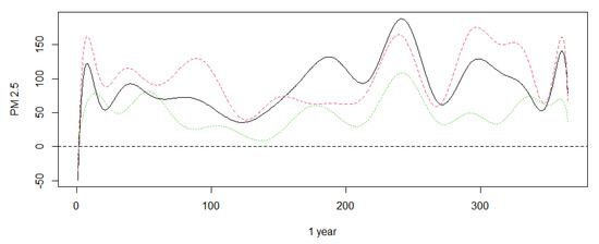
Figure 1. The mean PM 2.5 (μg/m${}^3$) of Beijing, Tianjin, and Shijiazhuang from December 2019 to January 2019. The black line stands for Beijing. The red dasehed line stands for Tianjin. The green dotted line stands for Shijiazhuang.

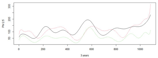
Figure 2. The mean PM 2.5 (μg/m${}^3$) of Beijing, Tianjin, and Shijiazhuang from December 2019 to January 2017. The black line stands for Beijing. The red asehed line stands for Tianjin. The green dotted line stands for Shijiazhuang.

It is obvious that PM 2.5 changes over individual periods. Here, we test whether there is a significant difference in PM 2.5 among the three cities using the method we proposed. First, the sample is divided into two data sets: the training sample is the dataset in 2017; the test sample is the dataset in 2018–2019. The principle components are adaptively based on the training sample. Then, the test statistic is constructed via the test sample and the principle components are selected by the training sample. To test whether there is significant difference in PM 2.5 between the three cities, we carry out permutations 1000 times within each group to calculate the rejection proportions; then, we obtain the p-value of the test. The results are shown in Table 10.

Table 10. p-value of two tests.

	Beijing vs. Tianjin		Beijing vs. Shijiazhuang		Tianjin vs. Shijiazhuang
Test	$N{T}_{1A}$	$N{T}_{2A}$	$N{T}_{1A}$	$N{T}_{2A}$	$N{T}_{1A}$	$N{T}_{2A}$
p-value	0.035	0.034	0.025	0.032	0.039	0.045

From Table 10, we can see that all p-values are less than 0.05. The tests are statistically significant and suggest that the average PM 2.5 in these three areas are different from each other at a 0.05 level of significance.

6. Conclusions and Discussions

In this paper, we consider the problem of testing the equality of mean functions in two random samples independently drawn from two functional random variables. We develop and study a novel testing procedure that has a more powerful ability to detect mean difference. In general, it includes two stages: first, splitting the sample into two parts and selecting principle components adaptively based on the first half-sample; then, constructing the test statistic based on another half-sample. An extensive simulation study is presented, which shows that the proposed test works very well in comparison with several other methods in a variety of settings. Our future project is to detect differences in the covariance functions of independent sample curves. There have been some approaches proposed so far to address this problem, for instance, the factor-based test proposed by [4] and the regularized M-test introduced by [16].

References

- Besse, P.; Ramsay, J. Principal components analysis of sampled functions. Psychometrika 1986, 51, 285–311. [Google Scholar] [CrossRef]
- Rice, J.A.; Silverman, B.W. Estimating the mean and covariance structure nonparametrically when the data are curves. J. R. Stat. Soc. Ser. B (Stat. Methodol.) 1991, 53, 233–243. [Google Scholar] [CrossRef]
- Ramsay, J.O.; Silverman, B.W. Functional Data Analysis; Springer Press: Berlin/Heidelberg, Germany, 2005. [Google Scholar]
- Ferraty, F.; Vieu, P.; Viguier-Pla, S. Factor-based comparison of groups of curves. Comput. Stat. Data Anal. 2007, 51, 4903–4910. [Google Scholar] [CrossRef]
- Horváth, L.; Kokoszka, P. Inference for Functional Data with Applications; Springer Press: Berlin/Heidelberg, Germany, 2012. [Google Scholar]
- Fan, J.Q.; Lin, S.K. Test of significance when data are curves. J. Am. Stat. Assoc. 1998, 93, 1007–1021. [Google Scholar] [CrossRef]
- Faraway, J.J. Regression analysis for a functional response. Technometrics 1997, 39, 254–261. [Google Scholar] [CrossRef]
- Zhang, C.Q.; Peng, H.; Zhang, J.T. Two samples tests for functional data. Commun. Stat.-Methods 2010, 39, 559–578. [Google Scholar] [CrossRef]
- Zhang, J.T. Statistical inferences for linear models with functional responses. Stat. Sin. 2011, 21, 1431–1451. [Google Scholar] [CrossRef]
- Zhang, J.T.; Liang, X. One-way ANOVA for functional data via globalizing the pointwise F-test. Scand. J. Stat. 2014, 45, 51–71. [Google Scholar] [CrossRef]
- Zhang, J.T.; Cheng, M.Y.; Wu, H.T.; Zhou, B. A new test for functional one-way ANOVA with applications to ischemic heart screening. Comput. Stat. Data Anal. 2019, 132, 3–17. [Google Scholar] [CrossRef]
- Wasserman, L.; Roeder, K. High dimensional variable selection. Ann. Stat. 2009, 37, 2178–2201. [Google Scholar] [CrossRef] [PubMed]
- Shen, Q.; Faraway, J.L. An F test for linear models with functional responses. Stat. Sin. 2004, 14, 1239–1257. [Google Scholar]
- Satterthwaites, F.E. Synthesis of variance. Psychometrika. 1941, 6, 309–3167. [Google Scholar] [CrossRef]
- Hall, P.; Hosseini-Nasab, M. On properties of functional principal components analysis. J. R. Stat. Soc. Ser. B (Stat. Methodol.) 2006, 68, 109–126. [Google Scholar] [CrossRef]
- Kraus, D.; Panaretos, V.M. Dispersion operators and resistant second-order functional data analysis. Biometrika 2012, 99, 813–832. [Google Scholar] [CrossRef]
- Kong, D.; Xue, K.; Yao, F.; Zhang, H.H. Partially functional linear regression in high dimensions (supplementary material). Biometrika 2016, 103, 147–159. [Google Scholar] [CrossRef]
- Shang, Y.L. A central limit theorem for randomly indexed m-dependent random variables. Filomat 2012, 26, 713–717. [Google Scholar] [CrossRef]
- Su, Y.R.; Di, C.Z.; Li, H. Hypothesis testing in functional linear models. Biometrics 2017, 73, 551–561. [Google Scholar] [CrossRef] [PubMed]
Publisher’s Note: MDPI stays neutral with regard to jurisdictional claims in published maps and institutional affiliations. |
© 2022 by the authors. Licensee MDPI, Basel, Switzerland. This article is an open access article distributed under the terms and conditions of the Creative Commons Attribution (CC BY) license (https://creativecommons.org/licenses/by/4.0/).