Abstract
Task scheduling is one of the most significant challenges in the cloud computing environment and has attracted the attention of various researchers over the last decades, in order to achieve cost-effective execution and improve resource utilization. The challenge of task scheduling is categorized as a nondeterministic polynomial time (NP)-hard problem, which cannot be tackled with the classical methods, due to their inability to find a near-optimal solution within a reasonable time. Therefore, metaheuristic algorithms have recently been employed to overcome this problem, but these algorithms still suffer from falling into a local minima and from a low convergence speed. Therefore, in this study, a new task scheduler, known as hybrid differential evolution (HDE), is presented as a solution to the challenge of task scheduling in the cloud computing environment. This scheduler is based on two proposed enhancements to the traditional differential evolution. The first improvement is based on improving the scaling factor, to include numerical values generated dynamically and based on the current iteration, in order to improve both the exploration and exploitation operators; the second improvement is intended to improve the exploitation operator of the classical DE, in order to achieve better results in fewer iterations. Multiple tests utilizing randomly generated datasets and the CloudSim simulator were conducted, to demonstrate the efficacy of HDE. In addition, HDE was compared to a variety of heuristic and metaheuristic algorithms, including the slime mold algorithm (SMA), equilibrium optimizer (EO), sine cosine algorithm (SCA), whale optimization algorithm (WOA), grey wolf optimizer (GWO), classical DE, first come first served (FCFS), round robin (RR) algorithm, and shortest job first (SJF) scheduler. During trials, makespan and total execution time values were acquired for various task sizes, ranging from 100 to 3000. Compared to the other metaheuristic and heuristic algorithms considered, the results of the studies indicated that HDE generated superior outcomes. Consequently, HDE was found to be the most efficient metaheuristic scheduling algorithm among the numerous methods researched.
MSC:
68W50; 90B36; 90C27
1. Introduction
Healthcare services (HCS) based on cloud computing and IoT are now seen as one of the most significant medical fields, due to the spread of epidemics and health crises, where the best use of HCS can save many lives [1]. Through the use of cloud computing, HCS users can gain access to online computing resources, such as software, hardware, and applications that are managed in accordance with their needs. As a result, cloud computing in the context of the Internet of Things has greatly benefited all users, especially those in the healthcare services industry who wish to deliver medical services via the Internet [2]. The rapid adoption and ease of use in all industries, the proliferation of the Internet of Things concept, and the continued advancement of infrastructure and technology will all increase user demand for cloud computing, doubling the volume of data and requests from users. Task scheduling becomes a more challenging issue. Delivering resources in accordance with user requests and upholding quality of service (QoS) requirements for the end-user is a demanding task [3].
Broadly speaking, cloud computing is made up of a large number of datacenters that house numerous physical machines (host). Each host runs several virtual machines (VMs) that are in charge of executing user tasks with varying quality of services (QoS). Users are able to gain access to cloud resources on a pay-as-you-go basis, through the use of cloud service providers [4]. An IoT environment connected to a cloud computing paradigm makes efficient use of the physical resources already available, thanks to virtualization technology. Thus, multiple users of healthcare services (HCS) can store and access a variety of medical resources using a single physical infrastructure, which includes both hardware and software. One of the most significant issues with healthcare services is the task scheduling problem (TSP), which causes users of healthcare services in a cloud computing environment to experience delays in receiving medical requests. The waiting period, the turnaround time for medical requests, CPU waste, and resource waste are some of the factors that contribute to the delay in processing medical requests. TSP is a NP-hard problem responsible for allocating computing resources to application tasks in an effective manner [2].
When the size of the tasks and the number of VMs both increase, the amount of computing time required to select the best scheduling for those tasks to the VMs increases exponentially. Some classic scheduling techniques, such as first come first served (FCFS), round-robin (RR), and shortest job first (SJF), are able to provide solutions to scheduling, but cannot fulfil the demands of cloud computing because its scheduling problem is NP-hard [5,6]. As traditional scheduling algorithms are unable to solve NP-hard optimization problems, more recently, modern optimization algorithms, also known as metaheuristic algorithms, have been used instead. These algorithms can produce optimal or near-optimal solutions in a reasonable amount of time compared to traditional scheduling algorithms.
Several metaheuristic algorithms have been employed for tackling task scheduling in cloud computing environments; for example, in [6], a new variant of the classic particle swarm optimization (PSO), namely ranging function and tuning function based PSO (RTPSO), was proposed, to achieve better task scheduling. In RTPSO, the inertia weight factors were improved to generate small and large values, for better local search and global search. In addition, RTPSO was integrated with the bat algorithm for further improvements; this variant was named RTPSO-B. Both RTPSO and RTPSO have been compared with various well-established algorithms, such as the genetic algorithm (GA), ant-colony optimization algorithm (ACO), and classical PSO. This comparison showed the efficiency of RTPSO-B in terms of its makespan, cost, and the utilization of resources.
The flower pollination algorithm (FPA) was also applied to tackle the task scheduling in cloud computing. Bezdan, T. et al. [7] improved the exploration operator of the classical FPA by replacing the worst individuals with new ones generated randomly within the search space, to avoid becoming stuck in local minima at the start of the optimization process. This improved FPA was called EEFPA and employed to find the best scheduling of tasks in cloud computing environments, which will minimize the makespan as a major objective. EEFPA was the best scheduler, compared to the other similar approaches considered in the study. Choudhary et al. [8] developed a task scheduling algorithm for bi-objective workflow scheduling in cloud computing that is based on hybridizing the gravitational search algorithm (GSA) and heterogeneous earliest finish time (HEFT); this algorithm was named as HGSA. This algorithm was developed in an effort to shorten the makespan and the computational cost. However, it is possible that GSA may not perform accurately for more complicated tasks.
Raghavan et al. [9] adapted the bat algorithm (BA) to tackle the task scheduling problem in cloud computing, with an objective function for reducing the total cost of the workflow. On the other hand, BA had a subpar performance in the high dimension [6]. Tawfeek et al. [10] devised ant colony optimization to deal with task scheduling in cloud computing, with the goal of reducing the makespan. This algorithm was compared to two traditional algorithms, such as FCFS and RR, and it performed better than both of them. The problem with this algorithm is that it converges slowly, and hence will take several iterations to obtain feasible solutions. Hamad and Omara [11] proposed a task scheduling algorithm based on the genetic algorithm (GA), to find the optimal assignment of tasks in cloud computing, which will optimize the makespan and cost, as well as the resource utilization.
The grey wolf optimizer (GWO) was proposed, to schedule the tasks in cloud computing to utilize the resources more efficiently and minimize the total completion time [12]. This algorithm was compared with several scheduling methods, such as the FCFS, ACO, performance budget ACO (PBACO), and min-max algorithms. The experimental findings showed that GWO was the best-performing scheduler and PBACO was the second best. However, the performance of GWO at large scale was not evaluated and, hence, it is not preferable when the number of tasks is at a large scale. Chen, X. et al. [13] presented a task scheduler based on the improved whale optimization algorithm (IWOA). The standard WOA was improved in IWOA using two factors, namely the nonlinear convergence factor and adaptive population size. IWOA was better than the compared algorithms in terms of accuracy and convergence speed when scheduling small-scale tasks or large-scale tasks in cloud computing environments.
Alsaidy, S.A. et al. [14] proposed two variants of PSO: The first, named LJFP-PSO, is based on initializing a population using a heuristic algorithm known as longest job to fastest processor (LJFP); while the second variant, known as MCT-PSO, is based on employing the minimum completion time (MCT) algorithm to initialize the population and to achieve a better makespan, total execution time, degree of imbalance, and total energy consumption when tackling the task scheduling problem in cloud computing. The glowworm swarm optimization (GSO) was used to solve the problem of task scheduling in cloud computing. The goal of this solution was to minimize the overall execution cost of jobs, while keeping the total completion time within the deadline [15]. According to the findings of a simulation, the GSO based task scheduling (GSOTS) algorithm achieved better results than the shortest task first (STF), the largest task first (LTF), and the particle swarm optimization (PSO) algorithms in terms of lowering the total completion time and the cost of executing tasks. There are several other metaheuristics-based task scheduling algorithms in the cloud computing environment, including the cuckoo search algorithm (CSA) [16], electromagnetism optimization (EMO) algorithm [17], sea lion optimization (SLO) algorithm [18], adaptive symbiotic organisms search (ASOS) [19], hybrid whale optimization algorithm (HWOA) [20], artificial flora optimization algorithm (AFOA) [21], modified particle swarm optimization (MPSO) [22], and differential evolution (DE) [23,24,25,26,27,28,29,30].
As mentioned, the task scheduling problem is classified as a nondeterministic polynomial time (NP)-hard problem and cannot be solved using traditional methods due to their inability to find a near-optimal solution in a reasonable time. Although, metaheuristic algorithms could have a significant effect when tackling these problems, they still suffer from falling into local minima and from a low convergence speed. As a result, a new task scheduler, known as hybrid differential evolution (HDE), is presented in this study, as a solution to the task scheduling challenge in the cloud computing environment. This scheduler is based on two proposed improvements to differential evolution. The first improvement is based on expanding the scaling factor to include dynamically generated numerical values based on the current iteration, in order to improve both the exploration and exploitation operators; the second improvement is intended to improve the exploitation operator of the classical DE, in order to achieve better results in fewer iterations. To demonstrate the efficacy of HDE, multiple tests were performed using randomly generated datasets and the CloudSim simulator. HDE was compared to a number of heuristic and metaheuristic algorithms, to show that it is a strong alternative for overcoming the task scheduling problem in cloud computing. The main contributions of this study are as follows:
- Improving the scaling factor and the exploitation operator of the classical DE, to propose a new task scheduler known as hybrid differential evolution for the challenge of task scheduling in the cloud computing environment.
- Conducting several experiments using randomly generated datasets and the CloudSim simulator, to verify the efficiency of HDE.
- The experimental findings show that HDE was the most effective metaheuristic scheduling algorithm among the compared approaches.
The remaining sections of this work are structured as follows: Section 2 describes the classical differential evolution, Section 3 presents the objective function formulation, Section 4 details the steps of the proposed algorithm, Section 5 depicts the results of the experiments and performance comparison, and Section 6 presents the conclusions drawn from this study, as well as observations regarding future research.
2. Task Scheduling in the Cloud Computing Environment
Cloud computing is made up of a large number of datacenters that house numerous physical machines (host). Each host runs several virtual machines (VMs) that are in charge of executing user tasks with varying quality of services (QoS). Figure 1 depicts the task scheduling in a cloud computing environment [4]. Supposing that there are n cloudlets (Tasks), , which are executed using m virtual machines (VMs), . These tasks have various lengths and the VMs are heterogonous in terms of bandwidth, RAM, and CPU time. The cloud broker makes a request to the cloud information service, to obtain details about the services needed to carry out the tasks it has been given, and then schedules the tasks on the services that have been found. The numerous variables and QoS criteria of the broker influence the choice of the tasks to be provided. The cloud broker is the key element of the task scheduling process, it mediates talks between the user and the provider and decides when to schedule tasks for certain resources. However, there are several issues that need to be considered. The tasks that users submit are first added to the top queue in the system and must wait while the resources are employed. As a result, the system’s queue grows longer, which lengthens the waiting period. However, a more effective approach than the first come first served (FCFS) principle should be used to manage this queue. Second, when the service provider manages the tasks, numerous parameters can be taken into account as multiobjective optimization or single objective optimization, such as the makespan, which directly affects resource consumption [4]. Therefore, a strong task scheduling algorithm should be created and implemented in the cloud broker, to not only meet the QoS requirements imposed by cloud users, but also to achieve good load balancing between the virtual machines, in order to improve resource utilization [4].
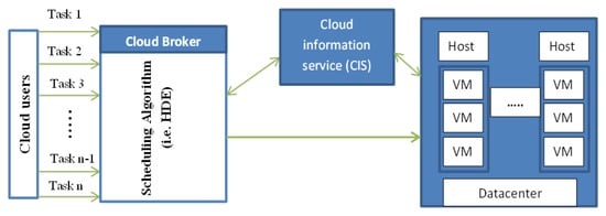
Figure 1.
Task scheduling process in the cloud computing environment [4].
3. Differential Evolution
Storn [31] presented a population-based optimization method dubbed differential evolution (DE). DE is comparable to genetic algorithms, in terms of its mutation, crossover, and selection operators. Before commencing the process of optimization, the differential evolution generates a set of solutions, referred to as individuals, each of which has D dimensions and is randomly dispersed within the search space of the optimization problem. This takes place before the optimization procedure begins. After that, as will become clear in the following paragraphs, the mutation and crossover operators are applied, in order to search through the space available in an effort to locate more effective solutions.
3.1. Mutation Operator
This operator is applied to generate a mutant vector for each solution in the population. There are several updating schemes that can be applied to generate the mutant vector, one of the most common schemes generates the mutant vector according to the following formula:
where , k, and j stand for the indices of three individuals picked randomly from the population at the current iteration t. F is a positive scaling factor that involves a constant value greater than 0.
3.2. Crossover Operator
After generating the mutant vector using the crossover operator under a crossover probability (CR), the trial vector is generated using both the mutant vector and the solution of the individual, according to the following equation:
where is a random integer generated between 1 and D, indicates the current dimension, and is a constant value between 0 and 1, which specifies the percentage of dimensions copied from the mutant vector to the trial vector.
3.3. Selection Operator
Finally, this operator is presented to compare the vector to vector , with the fittest being used in the next iteration. Generally, the selection operator for a minimization problem is mathematically formulated as follows:
4. Objective Function Formulation
Supposing that there are n cloudlets (Tasks), , which are executed using m virtual machines (VMs), . Then, the solutions obtained by a scheduler represent the assignment process of the tasks to the VMs in the order that will minimize the two objectives: makespan, and total execution time. Problems that have two or three objectives are classified as multiobjective. There are two methods, namely a priori or a posteriori, suggested to deal with multiobjective problems [32,33]. In the priori method, the multiobjective problems are treated as a single objective problem, by assigning a weight to each objective, based on the significance of each objective for the decision-makers. On the other hand, the posteriori method proposes that all objectives have the same significance, so it generates a set of solutions, namely non-dominated solutions, that trade off between different objectives. In this study, the priori approach was employed to convert the multiobjective problem into single objective using a weighting variable that includes a constant value generated between 0 and 1, to determine the importance of an objective, for example, the makespan, in the fitness function, and the complement of this variable () indicates the weight of the other objective. For instance, the objective function under this weighting variable is formulated as follows:
where represents the makespan objective, and stands for the total execution time. stands for the weighting variable, which is employed to convert this problem from multi-objective to single-objective, to become solvable using the met heuristic algorithms designed for single-objective problems, such as differential evolution. In the future, the posteriori approach will be applied to this problem, in an attempt to achieve better results for all objectives at the same time.
After describing the main components of the objective function, let us describe each one carefully. Starting with the makespan objective, at the beginning time, each has a variable assigned a value of 0, and then the tasks are distributed using a scheduler to those VMs. Each VM executes their assigned tasks and the execution time needed by each task to be executed under the VM is added to the variable . Finally, after finishing the tasks assigned to all VMs, the values stored in the variable for each VM are compared with each other, and the maximum value represents the makespan. Finally, the makespan, defined as the maximum of Et of all VMs, can be computed using the following expression:
The second objective is the total execution time consumed to complete the tasks assigned to all the VMs and can be computed according to the following formula:
Finally, the proposed algorithm described in the next section is employed to minimize the objective function described in Equation (4), to find the near-optimal scheduling of tasks that minimizes both the makespan and total execution time, hence providing a better quality of service to the users.
5. The Proposed Algorithm
This section presents the main steps employed to adapt the differential evolution for tackling the task scheduling problem in cloud computing; these steps are listed as follows: initialization, evaluation, adaptive mutation factor, and additional exploitation operator.
5.1. Initialization
Before starting the optimization process with any metaheuristic algorithm, a number N of solutions with n dimensions (each dimension represents a task in the scheduling problem) for each solution are defined and randomly initialized between 0 and m, to assign each task to a virtual machine. For example, Figure 2 presents a simple example, to illustrate how to represent a solution for the task scheduling problem. In this figure, we create a solution with 10 tasks, where n is 10, and randomly assign a VM to each task in this solution, where the number of available VMs is up to 7. From this figure, it is obvious that the virtual machine with an index of 2 will execute tasks 2 and 9, and the VM with an index of 0 will be assigned to execute tasks 1 and 5, while the other tasks, in order, will be assigned to the VMs: 1, 4, 3, 5, 6, and 5, respectively. In brief, the mathematical formula of the initialization step is defined as follows:
where stands for a vector involving decimal numbers generated randomly between 0 and 1, and indicates the multiplication operator. Following that step, the evaluation stage commences, to evaluate the quality of each solution and determine the best so-far solution that can reach the lowest value for the objective function described in Equation (4).
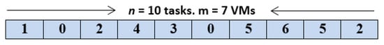
Figure 2.
A solution representation for task scheduling in cloud computing. This figure starts by numbering the cells with 0 and ends with an index of 9 for the last cell, such that the cell 0 indicates the first task, and the second cell indicates the second task, and so on.
5.2. Adaptive Scaling Factor (F)
The mutation stage in the differential evolution has a scaling factor, namely F, responsible for determining the step sizes. This factor in the classical DE algorithm includes a constant positive value, and this value is unchanged during the whole optimization process. Hence, if the population diversity is high and the value of this scaling factor is also high, the step size will take the solution a long distance from the current solution, this even occurs at the beginning of the optimization process, to encourage the algorithm to extensively explore the search space, to find the promising regions that might contain the best-so-far solution. Afterwards, the population diversity might be decreased when increasing the current iteration, while the scaling factor remains constant. However, what will happen if the population diversity remains high during the entire optimization process? Let us imagine together, if the population diversity remains high and the scaling factor is constant, then the generated step sizes are also high and, hence, the algorithm will always search for a better solution in regions far from the current solution, which might contain the near-optimal solution near to it. A similar problem occurs when the scaling factor is small and the population diversity is high. Therefore, in this study, we reformulated this factor to be dynamically updated according to the current iteration, to maximize the exploration operator of the classical DE algorithm at the beginning of the optimization process, and to search for the most promising region within the search space; and then, by increasing the current iteration, this exploration operator will be gradually converted into the exploitation operator, to focus more on this promising region, in order to achieve a better solution, in addition to accelerating the convergence. Based on this, the shortcomings of the classical DE with a constant scaling factor are largely avoided. Finally, the adaptive scaling factor is generated based on the current iteration, using the following formula:
where T indicates the maximum iteration, and t stands for the current iteration. is a predefined constant value.
5.3. Convergence Improvement Strategy
The mutation scheme described previously for generating the mutant vector in the classical DE is based on three solutions selected randomly from the current population. As a consequence of this, the exploration operator may be directed to explore the regions surrounding one of these solutions, despite the fact that the near-optimal solution may be in a region close to the best-so-far solution. Therefore, in this study, an additional strategy, namely a convergence improvement strategy (CIS), is proposed to exploit the regions around the best-so-far solution, to improve the convergence ability of the standard DE. This strategy in initially generates a vector, namely including numerical values generated around the best-so-far solution, using the following formula:
where indicates the best-so-far solution at the current iteration t, and and are two vectors including numerical values generated randomly between 0 and 1. Following this, another vector, namely a trial vector , will be generated based on conducting a crossover operation between and under a crossover probability (P) predetermined according to experiments. Briefly, the trial vector will be generated according to the following formula:
where is a numerical value generated randomly between 0 and 1. Finally, the fitness value of the trial vector, , will be compared with that of the current solution and if the fitness of this trial vector is better, then it will be used in the next iteration; otherwise, the current solution is retained in the next generation, even when reaching a better one. However, applying this strategy to all individuals in the population might deteriorate the exploration operator of the classical DE, because it might reduce the population diversity. Therefore, this strategy has to be applied to a number of the solutions, to avoid this shortcoming; this number is estimated using the following formula:
where is the number of individuals in the population, and is the percentage of the individuals that will be extracted to be updated using the convergence improvement strategy. Finally, the steps of the CIS strategy are listed in Algorithm 1.
| Algorithm 1. Convergence improvement strategy (CIS) |
| 1. for to 2. Generate the mutant vector using Equation (9) 3. for j = 0 to n 4. a number generated randomly between 0 and 1 5. ) 6. 7. else 8. 9. End if 10. end for 11. 12. = 13. end 14. Replace the best-so-far solution with if is better 15. end for |
5.4. Hybrid Differential Evolution
The classical DE is hybridized with the convergence improvement strategy and adaptive scaling factor, to produce a new variant dubbed hybrid differential evolution (HDE), having a better search ability, for a better solution when tackling the task scheduling in cloud computing. Another advantage of HDE is that it has the ability to accelerate the convergence speed in the direction of the near-optimal solution. The steps of HDE are described in Algorithm 2. This algorithm starts by initializing N solutions within the search space of the scheduling problem in cloud computing; the search space of this problem ranges between 0 and the number of virtual machines (m − 1). Then, the initialized solutions are evaluated, and the best-so-far solution that has the lowest fitness value is identified, to be employed for guiding some of the solutions within the optimization process towards a better solution. Line 3 within Algorithm 2 initializes the current iteration t with a value of 0. After this, the optimization process is triggered to update the initialized solutions to reach better solutions, whereby this process starts by defining the termination condition as shown in Line 4. Then, Lines 5–6 update the adaptive scaling factor, which is responsible for improving the exploration and exploitation capability of the proposed algorithm. Following this, updating of the solutions is implemented, to generate the trial vector based on both the current solution and the mutant vector. In the next step, this trial vector is compared with the current solution, to extract the one that will be preserved in the population for the next generation. This process is repeated until satisfying the termination condition. Finally, the flowchart of HDE is shown in Figure 3.
| Algorithm 2. Hybrid differential evolution (HDE) |
| 1. Initializes solutions, , using Equation (7) 2. Evaluate the initialized solutions and identified 3. 4. while (t < ) 5. Update using Equation (8) 6. 7. for to 8. Generate the mutant vector using Equation (1) 9. 10. for j = 0 to n 11. a number generated randomly between 0 and 1 12. ) 13. 14. else 15. 16. End if 17. end for 18. 19. = 20. end 21. Replace the best-so-far solution with if is better 22. end for 23. Updating solutions using the CIS algorithm (Algorithm 1) 24. 25. end while Return |
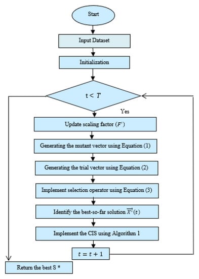
Figure 3.
The flowchart of the proposed algorithm: HDE (* is used to identify the best solution).
5.5. Time Complexity of HDE
In this part of the article, the time complexity is expressed using big-O notation, so that the superior speed of the suggested approach can be demostrated. To begin, the following are the primary factors that have the most significant impact on the acceleration of the proposed algorithm: the population size, N, the number of tasks, n, the maximum iteration, , and the time complexity of Algorithm 1. Generally, the time complexity of HDE can be expressed as follows:
The time complexity of the standard DE mostly depends solely on the first three factors: N, n, and T, as shown in Algorithm 2, which is formulated as follows:
The time complexity of the CIS also depends on the first three factors, with the exception of N, which is replaced by . In general, the time complexity of CIS can be expressed as follows:
By substitution, Equation (12) can be reformulated as follows:
From this equation, the term that has the highest growth rate is , because is always greater than . Therefore, the time complexity of HDE in big-O is .
6. Results and Simulation
Several experiments were conducted in this study to show the efficiency of the proposed algorithm: HDE was compared to several heuristic and metaheuristic approaches; the metaheuristic algorithms were the sine cosine algorithm (SCA) [34], whale optimization algorithm (WOA) [35], slime mold algorithm (SMA) [36], equilibrium optimizer (EO) [37], grey wolf optimizer (GWO) [38], and classical DE [39]; the heuristic algorithms were first come first served (FCFS) [40], round robin (RR) algorithm [41], and shortest job first (SJF) scheduler [40]. These algorithms were executed in 30 independent runs on datasets generated randomly, with the number of tasks ranging between 100 and 3000; these tasks are labeled as T100 for the task size 100, T200 for the task size 200, and so on. Five VMs were selected for scheduling these task data sets, where the communication time and execution time for each task were randomly generated to determine the ability of each VM to implement each task, while taking into consideration that the workload of this task is different of the other tasks. The performance evaluation metrics used in this study to compare the algorithms were the best, average, worst, and standard deviation of the obtained outcomes within 30 independent repetitions, in addition to a Wilcoxon rank sum test, which was employed to identify whether there were any differences between the outcomes obtained by the proposed and those of the rival optimizers. All of the algorithms were built using the programming language Java on a personal computer, which had the following capabilities: Windows 10 operating system, Intel® CoreTM i7-4700MQ processor running at 2.40 GHz, and 16 GB of memory installed.
The parameters of all the compared algorithms were set to the values found in the cited papers, to ensure a fair comparison. However, there were two main parameters that had to be the same for all the algorithms, and they were the population size (N), and the maximum number of iterations (T), which were set to 25 and 1500, respectively. Regarding the parameters of the classical DE and the proposed algorithm, HDE, several experiments were conducted to estimate the optimal value for each of their parameters. Broadly speaking, the classical DE has two main parameters: F and Cr, which were extracted according to several conducted experiments. From these experiments, it was observed that the best values for these parameters were 0.01 for Cr and 0.1 for the scaling factor (F). Regarding the parameter values of HDE, the Cr and parameters were set to the same values as the Cr and F in the classical DE. However, HDE has two additional parameters: and , which were estimated by conducting experiments. These experiments showed that the best values for these parameters, and were 0.01 and 0.2, respectively. Table 1 presents the parameter values of both HDE and DE.

Table 1.
Parameter settings of HDE and DE.
6.1. Comparison with Metaheuristic Algorithms
Due to the fact that meta-heuristic algorithms are stochastic optimization techniques, they require at least 10 separate runs to produce statistically significant results. In this study, each algorithm was run roughly thirty times independently, and the average results of each algorithm are reported. In Table A1 are shown the metrics of the best fitness values for each algorithm in the last iteration over all independent runs. These metrics include the mean, best, and worst values, as well as the standard deviation (SD). The top results in this table are highlighted in bold. This table demonstrates that HDE is comparable to DE and superior to all other algorithms for the 100-task size. With growing task sizes, HDE’s superiority becomes more apparent, and it may be the best option for any tasks with lengths more than 100. Additionally, to further show the efficiency of HDE, the average of the best, worst, and mean fitness values obtained for all the tasks sizes were computed and are presented in Figure 4, which affirms that HDE was the best for all shown metrics. Figure 5 shows the average (Avg) standard deviation (SD) obtained by each algorithm on all tasks sizes. Inspecting this figure shows that HDE was more stable than the other algorithms. After discussing the effectiveness of HDE in terms of the fitness value, we will move on to discuss its capacity to reduce the makespan in the next paragraph.
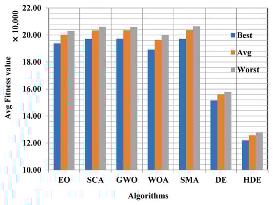
Figure 4.
Comparison among algorithms by fitness value.
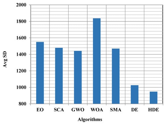
Figure 5.
Comparison in terms of average SD of the fitness values.
The metrics that represent the best makespan values for each method in the last iteration across all independent runs are presented in Table A2. The best, worst, and average values, as well as the standard deviation, are the metrics that were included in this study. The best outcomes are displayed in bold within this table. This table illustrates that HDE was superior to all other algorithms for the 100-task size and was on par with DE in terms of its performance. The superiority of HDE became more evident with increasing task sizes, and it is possible that it is the best choice for all tasks with lengths greater than 100. In addition, in order to demonstrate the effectiveness of HDE in a more comprehensive manner, the mean, best, and worst makespan values that were obtained for each of the different task sizes were computed and are shown in Figure 6. This figure demonstrates that HDE was the optimal method for each of the metrics that are presented. Figure 7 displays the average of the standard deviation (SD) values that were obtained by each algorithm for all task sizes. Taking a closer look at this figure reveals that HDE was far more reliable than the other algorithms. Now we have finished talking about how effective HDE was in terms of the fitness value and makespan, in the following paragraph, we will move on to talking about how it had the ability to reduce the total execution time required by all VMs, until finishing the tasks that had been given to them.
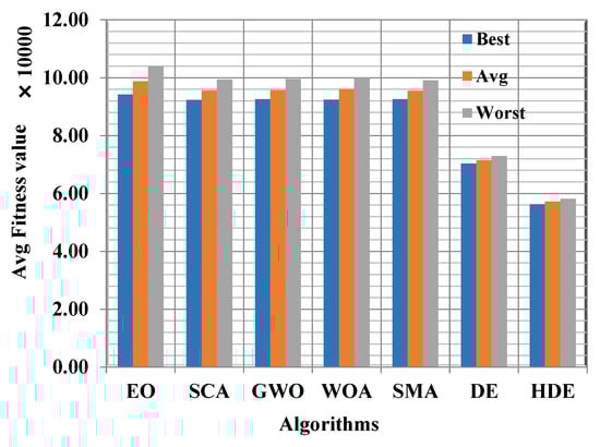
Figure 6.
Comparison among algorithms by makespan.
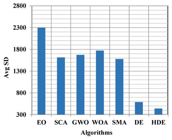
Figure 7.
Comparison with metaheuristics in terms of the average SD of makespan.
The average, worst, best, and SD values obtained as a result of analyzing the total execution time values obtained by the various investigated metaheuristic algorithms within 30 independent runs are reported in Table A3. Based on the results in this table, it is clear that HDE performed just as well as DE and was superior to all the other algorithms when it comes to a size of 100 tasks. It is probable that HDE is the optimal option for all tasks with lengths that are larger than 100. The superiority of HDE became more readily apparent as the size of the tasks was increased. The average of the mean, best, and worst total execution values that were obtained for each of the various task sizes was computed and are given in Figure 8, in order to showcase the efficacy of HDE in a more thorough manner. This was done in order to prove that HDE was effective. This figure illustrates that HDE was the best strategy for each of the metrics that are presented. Figure 9 depicts the average of the standard deviation (SD) values that were obtained using each method for all of the various task sizes. When taking a closer look at this figure, it can be noticed that HDE was significantly more trustworthy than any of the other algorithms. Finally, from all the previous experiments and discussions, it is concluded that HDE is a strong alternative scheduler to find the near-optimal scheduling of tasks in cloud computing, with the aim of minimizing both the makespan and the total execution time.
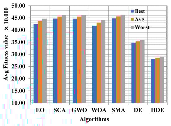
Figure 8.
Comparison among algorithms for the total execution time.
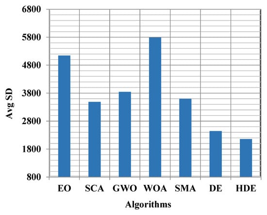
Figure 9.
Comparison in terms of the average SD of total execution time.
Table A4 compares the proposed HDE algorithm to the other types using a Wilcoxon rank-sum test with 5% as the level of confidence [42]. The null hypothesis and the alternative hypothesis were both tested in this experiment. The null hypothesis suggests that there is no difference between the two methods being compared; this hypothesis is true when the p-value shown in Table A4 is greater than the confidence level. In contrast, the alternative hypothesis asserts that there is a difference between the results obtained using a pair of algorithms; this hypothesis is supported when p-value is less than the confidence level. Table A4 displays the results of comparing HDE to the other algorithms evaluated in this test. According to this table, the alternative hypothesis holds true in all instances, highlighting the difference between the outcomes of the proposed algorithm and those of other algorithms.
The boxplot represented in Figure 10 is discussed in this paragraph. The boxplot shows a five-number summary, including the lowest, maximum, median, and the first and third quartiles for the fitness values achieved by each algorithm during 30 independent runs. Examining this figure demonstrates that HDE was superior in terms of all five-number summaries for all of the investigated task lengths.
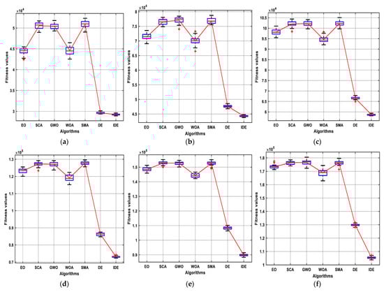
Figure 10.
Comparison among algorithms in terms of the Boxplot: (a) Comparison for the task size of 200; (b) Comparison for the task size of 300; (c) Comparison for the task size of 400; (d) Comparison for the task size of 500; (e) Comparison for the task size of 600; (f) Comparison for the task size of 700.
Finally, HDE and the other algorithms were compared based on their respective convergence rates for the fitness function. On the basis of the convergence rates obtained by each algorithm, and presented in Figure 11, for task lengths 100, 200, 300, 400, 500, 600, 700, 800, and 900, HDE achieved superior convergence to the optimal solution for all depicted task lengths. Figure 12 shows a comparison among the algorithms in terms of CPU time. The figure provides the total CPU time in seconds for running each algorithm with different task sizes. HDE had a slightly higher computational cost than traditional DE, but it can provide a better QoS to users, because it can achieve a smaller makepan value for the majority of task sizes.
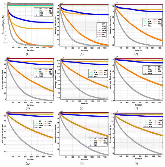
Figure 11.
Comparison of algorithms in terms of convergence speed: (a) Comparison for the task size of 100; (b) Comparison for the task size of 200; (c) Comparison for the task size of 300; (d) Comparison for the task size of 400; (e) Comparison for the task size of 500; (f) Comparison for the task size of 600; (g) Comparison for the task size of 700; (h) Comparison for the task size of 800; (i) Comparison for the task size of 900.
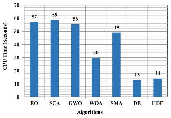
Figure 12.
Comparison of algorithms in terms of CPU time.
6.2. Comparison with Some Heuristic Algorithms
In this section, the proposed algorithm is compared with some well-known heuristic schedulers, such as FCFS, SJF, and round robin, to further verify the superiority of HDE in tackling the task scheduling problem in cloud computing. The results of each method were independently tested around thirty times. In Table A5, the average, worst, and best values are shown, as well as the standard deviations, that were achieved by the proposed approach and by each heuristic algorithm for each task size. The results of this table show that HDE performed significantly better than any of the heuristic algorithms. In addition, in order to demonstrate the effectiveness of HDE in a more comprehensive manner, the average of the best, worst, and mean makespan values obtained for all task sizes were computed and are shown in Figure 13. This figure confirms that HDE was the most effective method for all of the metrics presented. Figure 14 depicts the average (Avg) and standard deviation (SD) of the makespan values obtained by each algorithm across all task sizes. Taking a closer look at this figure reveals that HDE was significantly more reliable than the other algorithms. It is worth mentioning that the heuristic algorithms have a negligible computation cost compared to metaheuristic algorithms, but their solutions are poor when compared to the metaheuristics algorithms. As a result, to provide a better quality of service to the users, while excluding the computational cost, the proposed algorithm is the most effective. On the other hand, if the computational cost is more important than the quality of service, then the heuristic algorithms, specifically FCFS, are the best.
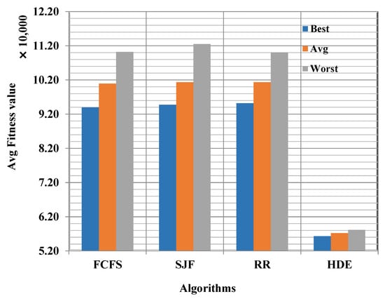
Figure 13.
Comparison among algorithms for makespan.
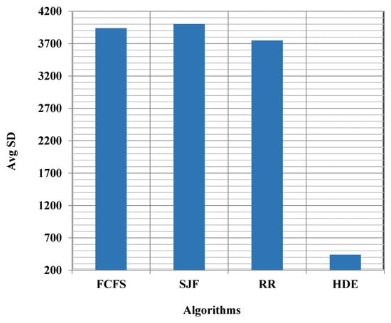
Figure 14.
Comparison with heuristic algorithms in terms of the average SD of makespan.
6.3. Simulation Results
The CloudSim platform was utilized in order to carry out simulations of the task scheduling process. Researchers from all over the world make use of the CloudSim platform because it is a full-fledged simulation toolset that enables modelling and simulation of real-world cloud infrastructure and application provisioning [12]. In this paper, CloudSim was provided with the parameters settings described in Table 2. In addition, the number of tasks ranged between 100 and 1000, with a step 100, to check the scalability of the proposed algorithm in comparison to the other metaheuristic algorithms. After conducting the simulation process, the makespan values obtained under various metaheuristic algorithms implemented within the Cloudsim platform are presented in Table 3 for each task size. Inspecting this table shows the effectiveness of HDE in comparison to the other algorithms, since it had the lowest makespan values for all the task sizes. This is confirmed by the last row in the same table which contains the average of each column within the table; this row reveals that HDE could achieve average makespan values up to 151,479.2179, which is the smallest in comparison to the others in the same row.
Table 2.
Parameters of the CloudSim platform.
Table 3.
Comparison among algorithms in terms of the makespan values for the Cloudsim-based simulation.
7. Conclusions and Future Work
This paper presents a new scheduler, namely hybrid differential evolution (HDE), for the task scheduling problem in the cloud computing environment. This scheduler is based on two proposed improvements to the classical differential evolution. The first improvement is based on improving the scaling factor, to involve numerical values generated dynamically based on the current iteration, to improve both the exploration and exploitation operators; meanwhile the second improvement is designed to further improve the exploitation operator of the classical DE, to achieve better outcomes in a smaller number of iterations. Several experiments were performed using randomly generated datasets and the CloudSim simulator, to verify the efficiency of HDE. In addition, HDE was compared with several heuristic and metaheuristic algorithms, such as the slime mold algorithm (SMA), equilibrium optimizer (EO), sine cosine algorithm (SCA), whale optimization algorithm (WOA), grey wolf optimizer (GWO), classical DE, first come first served (FCFS), round robin (RR) algorithm, and shortest job first (SJF) scheduler. Makespan and total execution time values were obtained for various task sizes, ranging between 100 and 3000, during the experiments. The findings of the experiments indicated that HDE produced effective results when compared to the other metaheuristic and heuristic algorithms that were investigated. As a result, HDE was the most effective metaheuristic scheduling algorithm among the many approaches that were investigated. In future work, HDE will be employed to tackle several other optimization problems, such as the DNA fragment assembly problem, image segmentation problem, 0-1 knapsack problem, and task scheduling problem in fog computing.
Author Contributions
Conceptualization, M.A.-B., R.M. and W.A.E.; methodology, M.A.-B., R.M., W.A.E. and K.M.S.; software, M.A.-B., R.M. and W.A.E.; validation, M.A.-B., R.M., W.A.E., M.S. and K.M.S.; formal analysis, M.A.-B., R.M., W.A.E. and K.M.S.; investigation, M.A.-B., R.M., W.A.E. and K.M.S.; data curation, M.A.-B., R.M., W.A.E., M.S. and K.M.S.; writing—original draft preparation, M.A.-B., R.M and W.A.E.; writing—review and editing M.A.-B., R.M., W.A.E., M.S. and K.M.S.; visualization, M.A.-B., R.M., W.A.E. and K.M.S.; supervision, M.A.-B.; funding acquisition, M.S. All authors have read and agreed to the published version of the manuscript.
Funding
This research received no external funding.
Data Availability Statement
Not applicable.
Conflicts of Interest
The authors declare no conflict of interest.
Appendix A. Comparison with Some Heuristic and Metaheuristic Algorithms
Table A1.
Comparison with some metaheuristic algorithms for the fitness values.
Table A1.
Comparison with some metaheuristic algorithms for the fitness values.
| TS | EO | SCA | GWO | WOA | SMA | DE | HDE | |
|---|---|---|---|---|---|---|---|---|
| T100 | Best | 18,265.116 | 24,611.809 | 24,088.115 | 19,972.837 | 24,613.264 | 15,150.553 | 15,137.092 |
| Avg | 19,571.000 | 25,528.000 | 25,375.000 | 21,258.000 | 25,704.000 | 15,196.000 | 15,274.000 | |
| Worst | 21,498.010 | 26,402.739 | 26,051.051 | 22,205.813 | 26,752.888 | 15,257.978 | 15,558.919 | |
| SD | 713.524 | 463.258 | 424.731 | 558.666 | 521.104 | 30.572 | 91.663 | |
| T200 | Best | 42,426.362 | 48,950.808 | 49,292.426 | 42,546.316 | 49,025.035 | 29,373.841 | 28,909.445 |
| Avg | 44,394.000 | 50,538.000 | 50,422.000 | 44,527.000 | 50,967.000 | 29,627.000 | 29,231.000 | |
| Worst | 45,476.446 | 51,690.914 | 51,790.672 | 46,474.198 | 52,320.876 | 30,126.857 | 29,605.929 | |
| SD | 828.993 | 778.633 | 618.134 | 1021.092 | 811.779 | 184.835 | 184.273 | |
| T300 | Best | 69,067.191 | 74,866.300 | 74,062.850 | 66,476.677 | 75,546.109 | 46,803.516 | 43,810.658 |
| Avg | 71,383.000 | 76,534.000 | 77,081.000 | 69,943.000 | 76,864.000 | 47,615.000 | 44,284.000 | |
| Worst | 73,579.777 | 78,080.754 | 78,483.051 | 73,289.182 | 78,743.006 | 48,568.449 | 44,801.076 | |
| SD | 1134.455 | 867.221 | 1041.396 | 1443.511 | 874.786 | 430.618 | 255.008 | |
| T400 | Best | 95,440.911 | 98,432.590 | 99,668.262 | 92,093.906 | 99,673.090 | 64,938.822 | 58,147.125 |
| Avg | 98,176.000 | 102,045.000 | 102,211.000 | 94,585.000 | 102,252.000 | 66,478.000 | 58,708.000 | |
| Worst | 101,000.236 | 104,376.315 | 104,112.797 | 98,252.609 | 105,053.622 | 67,814.981 | 59,395.477 | |
| SD | 1348.619 | 1285.976 | 1075.139 | 1514.400 | 1256.732 | 701.588 | 323.410 | |
| T500 | Best | 120,119.573 | 123,408.542 | 123,758.958 | 115,201.767 | 125,660.988 | 84,738.675 | 72,282.977 |
| Avg | 123,307.000 | 127,282.000 | 127,133.000 | 119,111.000 | 127,791.000 | 86,195.000 | 73,084.000 | |
| Worst | 125,568.639 | 129,252.182 | 129,228.583 | 122,399.771 | 129,623.395 | 87,526.696 | 74,219.055 | |
| SD | 1440.633 | 1187.152 | 1291.705 | 1697.175 | 919.858 | 809.404 | 463.869 | |
| T600 | Best | 145,919.544 | 149,987.437 | 150,121.722 | 142,155.751 | 148,997.028 | 106,351.443 | 88,355.874 |
| Avg | 148,462.000 | 152,813.000 | 152,648.000 | 144,351.000 | 152,621.000 | 108,316.000 | 89,783.000 | |
| Worst | 151,270.871 | 155,095.573 | 154,638.766 | 146,586.770 | 155,053.210 | 110,123.047 | 91,415.701 | |
| SD | 1292.904 | 1264.745 | 1003.265 | 1346.239 | 1435.543 | 980.036 | 646.848 | |
| T700 | Best | 171,248.666 | 174,068.432 | 172,269.168 | 162,866.453 | 171,421.871 | 128,092.342 | 103,753.063 |
| Avg | 173,404.000 | 176,365.000 | 176,581.000 | 168,979.000 | 176,401.000 | 129,789.000 | 105,350.000 | |
| Worst | 177,380.381 | 178,450.265 | 180,508.600 | 174,375.747 | 179,642.085 | 131,573.149 | 107,198.432 | |
| SD | 1388.031 | 1166.368 | 1703.244 | 2689.929 | 1563.520 | 800.844 | 750.188 | |
| T800 | Best | 197,457.353 | 200,198.689 | 199,590.942 | 190,388.160 | 200,882.988 | 149,519.095 | 117,842.491 |
| Avg | 201,048.000 | 203,729.000 | 203,492.000 | 195,286.000 | 203,970.000 | 152,379.000 | 120,551.000 | |
| Worst | 204,902.594 | 206,534.694 | 207,776.148 | 200,825.073 | 206,878.190 | 154,292.126 | 123,731.662 | |
| SD | 1683.470 | 1656.565 | 1899.381 | 2196.411 | 1523.478 | 1199.194 | 1176.508 | |
| T900 | Best | 223,704.461 | 226,558.832 | 226,409.487 | 217,996.729 | 226,114.867 | 172,082.041 | 135,865.435 |
| Avg | 226,980.000 | 229,924.000 | 230,362.000 | 222,388.000 | 229,935.000 | 174,181.000 | 137,631.000 | |
| Worst | 229,921.195 | 233,724.590 | 233,488.493 | 225,639.051 | 233,651.341 | 176,793.002 | 139,246.915 | |
| SD | 1673.049 | 1834.109 | 1787.159 | 1794.545 | 1706.194 | 1229.686 | 863.086 | |
| T1000 | Best | 247,875.320 | 249,814.443 | 250,647.285 | 242,389.074 | 250,741.549 | 194,418.935 | 152,868.454 |
| Avg | 251,792.000 | 253,414.000 | 253,521.000 | 246,631.000 | 253,945.000 | 196,598.000 | 155,350.000 | |
| Worst | 254,529.450 | 257,498.878 | 256,169.629 | 250,551.728 | 256,575.530 | 198,807.888 | 157,666.486 | |
| SD | 1615.810 | 1823.711 | 1598.983 | 1604.413 | 1469.167 | 1146.393 | 1329.473 | |
| T1200 | Best | 272,161.798 | 275,012.674 | 273,177.920 | 266,930.950 | 275,918.637 | 215,439.409 | 168,684.208 |
| Avg | 276,665.000 | 278,762.000 | 278,623.000 | 272,150.000 | 279,459.000 | 218,984.000 | 172,241.000 | |
| Worst | 279,816.799 | 282,024.626 | 282,025.504 | 277,318.739 | 281,727.579 | 220,993.332 | 175,396.503 | |
| SD | 1654.505 | 1979.462 | 2136.547 | 2217.506 | 1530.659 | 1458.254 | 1543.670 | |
| T1500 | Best | 297,700.056 | 301,895.921 | 300,516.283 | 289,987.072 | 301,107.227 | 240,484.692 | 188,831.791 |
| Avg | 302,389.000 | 304,816.000 | 305,067.000 | 297,244.000 | 304,918.000 | 243,074.000 | 192,415.000 | |
| Worst | 306,262.646 | 306,790.966 | 307,331.538 | 300,181.346 | 308,731.491 | 245,362.366 | 195,299.922 | |
| SD | 2105.256 | 1457.285 | 1731.171 | 2124.410 | 1735.142 | 1424.956 | 1558.728 | |
| T2000 | Best | 324,305.532 | 328,468.897 | 328,886.931 | 318,205.762 | 325,580.330 | 265,211.125 | 209,699.639 |
| Avg | 329,160.000 | 331,652.000 | 331,396.000 | 323,903.000 | 330,530.000 | 268,229.000 | 212,927.000 | |
| Worst | 332,916.550 | 335,830.685 | 334,367.352 | 329,829.207 | 334,457.438 | 270,526.428 | 216,136.640 | |
| SD | 2167.010 | 1789.437 | 1634.825 | 2473.637 | 1970.316 | 1248.839 | 1521.468 | |
| T2500 | Best | 349,691.604 | 350,883.081 | 352,358.092 | 343,367.024 | 351,080.666 | 286,532.304 | 224,756.706 |
| Avg | 353,786.000 | 355,235.000 | 355,558.000 | 348,528.000 | 355,706.000 | 289,731.000 | 228,761.000 | |
| Worst | 357,011.837 | 359,479.690 | 358,061.266 | 352,923.652 | 360,249.932 | 292,567.734 | 233,007.159 | |
| SD | 1762.202 | 1972.154 | 1614.774 | 2190.929 | 2216.089 | 1639.396 | 1996.000 | |
| T3000 | Best | 374,687.613 | 374,116.100 | 378,044.013 | 368,165.769 | 374,348.289 | 308,332.567 | 247,888.247 |
| Avg | 380,344.000 | 382,277.000 | 382,538.000 | 375,197.000 | 381,730.000 | 314,351.000 | 250,242.000 | |
| Worst | 384,988.196 | 386,465.343 | 386,075.515 | 380,355.337 | 386,174.587 | 317,335.349 | 253,382.767 | |
| SD | 2444.072 | 2658.810 | 2068.051 | 2672.652 | 2505.108 | 2100.287 | 1509.886 |
The bold values indicate the best values.
Table A2.
Comparison among algorithms for the makespan values.
Table A2.
Comparison among algorithms for the makespan values.
| TS | EO | SCA | GWO | WOA | SMA | DE | HDE | |
|---|---|---|---|---|---|---|---|---|
| T100 | Best | 9438.672 | 11,947.637 | 12,712.777 | 10,884.463 | 11,975.781 | 6944.882 | 6944.882 |
| Avg | 10,516.000 | 12,859.000 | 13,645.000 | 11,750.000 | 12,807.000 | 7010.000 | 7013.000 | |
| Worst | 12,883.040 | 14,826.337 | 15,092.457 | 12,654.819 | 13,823.656 | 7137.436 | 7129.975 | |
| SD | 653.494 | 683.114 | 571.680 | 447.619 | 553.510 | 40.354 | 43.224 | |
| T200 | Best | 22,547.028 | 23,002.456 | 23,210.790 | 21,671.230 | 23,050.308 | 13,431.827 | 13,185.932 |
| Avg | 24,472.000 | 24,684.000 | 25,148.000 | 23,759.000 | 24,660.000 | 13,594.000 | 13,348.000 | |
| Worst | 26,066.689 | 26,378.086 | 27,355.248 | 25,403.570 | 26,345.011 | 14,041.473 | 13,538.203 | |
| SD | 829.519 | 960.601 | 1163.940 | 882.523 | 888.877 | 129.345 | 91.631 | |
| T300 | Best | 36,947.699 | 34,559.880 | 34,731.946 | 34,232.690 | 35,303.618 | 21,389.497 | 19,972.977 |
| Avg | 38,439.000 | 36,801.000 | 37,327.000 | 36,425.000 | 36,938.000 | 21,878.000 | 20,194.000 | |
| Worst | 40,431.356 | 38,900.228 | 41,404.623 | 39,453.807 | 39,017.019 | 22,363.346 | 20,472.578 | |
| SD | 976.881 | 909.559 | 1666.857 | 1116.936 | 854.587 | 228.565 | 127.459 | |
| T400 | Best | 48,955.367 | 45,647.852 | 46,915.152 | 46,597.809 | 46,455.141 | 29,617.292 | 26,444.417 |
| Avg | 51,779.000 | 48,799.000 | 48,556.000 | 48,947.000 | 48,528.000 | 30,500.000 | 26,731.000 | |
| Worst | 55,070.040 | 51,597.179 | 52,287.562 | 51,820.391 | 50,765.243 | 31,290.145 | 27,121.008 | |
| SD | 1509.922 | 1383.763 | 1272.435 | 1346.970 | 1208.233 | 400.760 | 161.878 | |
| T500 | Best | 61,001.750 | 57,658.760 | 57,566.241 | 58,607.792 | 59,016.133 | 38,674.036 | 32,957.020 |
| Avg | 64,916.000 | 60,584.000 | 60,244.000 | 60,900.000 | 60,608.000 | 39,487.000 | 33,269.000 | |
| Worst | 67,560.243 | 64,112.117 | 62,532.085 | 63,017.762 | 62,815.301 | 40,093.788 | 33,819.042 | |
| SD | 1560.291 | 1421.079 | 1234.821 | 1193.972 | 940.158 | 417.670 | 224.071 | |
| T600 | Best | 73,229.925 | 69,331.153 | 69,586.533 | 69,647.496 | 68,512.668 | 48,727.438 | 40,158.207 |
| Avg | 76,445.000 | 72,328.000 | 72,067.000 | 72,844.000 | 72,158.000 | 49,612.000 | 40,845.000 | |
| Worst | 80,532.895 | 77,530.876 | 75,054.437 | 77,227.793 | 749,26.269 | 50,879.790 | 41,495.153 | |
| SD | 1701.605 | 1594.430 | 1333.427 | 1659.749 | 1515.736 | 541.237 | 292.474 | |
| T700 | Best | 84,822.010 | 81,046.928 | 80,384.642 | 79,314.560 | 79,554.619 | 58,557.297 | 47,217.700 |
| Avg | 88,690.000 | 83,167.000 | 83,246.000 | 84,249.000 | 82,848.000 | 59,386.000 | 47,921.000 | |
| Worst | 93,188.460 | 85,347.315 | 86,615.127 | 87,747.237 | 86,999.870 | 60,544.019 | 48,675.067 | |
| SD | 2128.515 | 1231.305 | 1612.775 | 1790.731 | 1662.438 | 460.926 | 330.657 | |
| T800 | Best | 96,380.442 | 92,521.921 | 92,321.704 | 91,262.035 | 93,067.232 | 68,677.526 | 53,779.212 |
| Avg | 100,603.000 | 95,559.000 | 95,873.000 | 96,413.000 | 96,213.000 | 69,688.000 | 54,867.000 | |
| Worst | 106,564.905 | 98,404.951 | 99,524.222 | 100,831.242 | 101,401.679 | 70,661.792 | 56,282.630 | |
| SD | 2414.587 | 1423.826 | 2017.753 | 2166.084 | 2066.140 | 513.065 | 545.623 | |
| T900 | Best | 108,229.730 | 103,645.560 | 104,628.113 | 105,548.365 | 104,277.133 | 78,792.104 | 61,758.499 |
| Avg | 113,582.000 | 107,669.000 | 107,999.000 | 109,495.000 | 107,688.000 | 79,775.000 | 62,626.000 | |
| Worst | 120,148.440 | 112,419.694 | 114,072.174 | 111,749.833 | 111,998.498 | 81,359.462 | 63,399.167 | |
| SD | 2850.589 | 2007.737 | 2051.189 | 1641.801 | 1715.424 | 624.858 | 408.529 | |
| T1000 | Best | 118,736.975 | 115,138.440 | 115,625.172 | 116,100.770 | 116,206.118 | 88,832.449 | 69,515.446 |
| Avg | 123,279.000 | 118,956.000 | 119,125.000 | 120,234.000 | 118,929.000 | 90,012.000 | 70,684.000 | |
| Worst | 129,183.176 | 122,706.004 | 122,156.907 | 124,499.643 | 124,431.728 | 93,798.984 | 71,658.817 | |
| SD | 2489.881 | 1666.849 | 1659.843 | 2417.331 | 1778.316 | 874.974 | 620.257 | |
| T1200 | Best | 129,795.983 | 126,954.152 | 126,249.252 | 127,570.871 | 127,972.633 | 98,118.160 | 76,652.611 |
| Avg | 134,908.000 | 130,688.000 | 130,519.000 | 132,035.000 | 130,779.000 | 100,158.000 | 78,409.000 | |
| Worst | 141,397.459 | 135,719.950 | 134,650.907 | 139,766.474 | 136,984.431 | 101,266.796 | 79,725.686 | |
| SD | 2309.279 | 1870.231 | 2018.753 | 2729.933 | 2251.355 | 774.466 | 705.732 | |
| T1500 | Best | 138,804.579 | 138,898.602 | 139,292.203 | 139,693.196 | 138,606.731 | 109,581.936 | 85,953.213 |
| Avg | 145,796.000 | 142,250.000 | 142,775.000 | 143,012.000 | 142,380.000 | 111,340.000 | 87,520.000 | |
| Worst | 153,587.370 | 145,607.443 | 150,992.953 | 147,576.341 | 146,704.239 | 114,272.274 | 89,009.316 | |
| SD | 3283.758 | 1526.583 | 2390.077 | 1991.793 | 1614.124 | 1072.070 | 721.108 | |
| T2000 | Best | 151,784.006 | 151,264.096 | 150,594.060 | 149,722.432 | 151,191.472 | 121,190.063 | 95,349.975 |
| Avg | 157,611.000 | 155,420.000 | 154,648.000 | 155,396.000 | 154,322.000 | 122,618.000 | 96,813.000 | |
| Worst | 166,344.617 | 160,214.293 | 159,508.888 | 161,005.512 | 159,349.068 | 123,936.506 | 98,162.927 | |
| SD | 3677.971 | 2504.031 | 2137.704 | 2628.660 | 1852.858 | 637.741 | 698.603 | |
| T2500 | Best | 160,529.235 | 160,637.179 | 162,072.574 | 161,144.576 | 161,100.021 | 130,477.400 | 102,136.632 |
| Avg | 169,506.000 | 165,738.000 | 166,038.000 | 166,450.000 | 165,581.000 | 132,810.000 | 104,022.000 | |
| Worst | 179,163.135 | 171,771.518 | 169,385.501 | 173,371.558 | 169,513.351 | 134,690.256 | 106,190.281 | |
| SD | 4406.047 | 2343.341 | 1588.846 | 2503.864 | 2282.155 | 925.081 | 933.183 | |
| T3000 | Best | 172,070.805 | 172,887.505 | 173,311.921 | 174,193.094 | 173,026.585 | 142,122.392 | 112,625.384 |
| Avg | 181,066.000 | 177,940.000 | 178,119.000 | 178,707.000 | 177,882.000 | 144,111.000 | 113,811.000 | |
| Worst | 187,904.224 | 184,878.509 | 182,574.837 | 183,514.827 | 181,860.483 | 147,212.405 | 115,274.338 | |
| SD | 3690.548 | 2693.045 | 2364.794 | 2069.685 | 2493.556 | 1188.774 | 701.579 |
The bold values indicate the best values.
Table A3.
Comparison among algorithms for total execution time.
Table A3.
Comparison among algorithms for total execution time.
| TS | EO | SCA | GWO | WOA | SMA | DE | HDE | |
|---|---|---|---|---|---|---|---|---|
| T100 | Best | 38,115.003 | 50,570.643 | 49,339.028 | 40,070.182 | 52,314.209 | 34,167.699 | 34,184.939 |
| Avg | 40,701.000 | 55,087.000 | 52,746.000 | 43,443.000 | 55,795.000 | 34,298.000 | 34,550.000 | |
| Worst | 43,980.020 | 57,190.514 | 56,010.407 | 46,197.991 | 57,836.610 | 34,461.035 | 35,226.454 | |
| SD | 1093.390 | 1509.796 | 1560.900 | 1514.701 | 1342.057 | 74.832 | 228.008 | |
| T200 | Best | 86,987.143 | 105,072.258 | 103,976.815 | 87,848.691 | 108,440.506 | 66,302.970 | 65,521.241 |
| Avg | 90,879.000 | 110,862.000 | 109,394.000 | 92,988.000 | 112,350.000 | 67,038.000 | 66,290.000 | |
| Worst | 95,059.361 | 114,933.861 | 113,761.796 | 98,376.422 | 115,141.894 | 67,843.837 | 67,119.554 | |
| SD | 2114.152 | 2408.720 | 2660.714 | 2577.679 | 1907.367 | 414.783 | 429.283 | |
| T300 | Best | 140,739.328 | 164,556.186 | 161,414.947 | 141,130.001 | 165,788.713 | 105,870.995 | 99,269.263 |
| Avg | 148,252.000 | 169,244.000 | 169,843.000 | 148,151.000 | 170,026.000 | 107,669.000 | 100,496.000 | |
| Worst | 151,986.556 | 172,666.021 | 175,454.835 | 155,885.560 | 174,514.307 | 109,713.690 | 101,829.995 | |
| SD | 2883.541 | 1929.747 | 3292.297 | 3351.197 | 2029.973 | 1011.817 | 610.498 | |
| T400 | Best | 197,268.901 | 220,893.125 | 220,314.876 | 194,313.759 | 223,848.304 | 146,681.999 | 132,120.112 |
| Avg | 206,434.000 | 226,286.000 | 227,406.000 | 201,072.000 | 227,607.000 | 150,428.000 | 133,321.000 | |
| Worst | 212,775.565 | 233,178.780 | 233,772.309 | 213,052.367 | 234,076.000 | 153,333.362 | 134,949.635 | |
| SD | 3429.782 | 2590.382 | 2766.779 | 4734.105 | 2765.688 | 1528.621 | 718.928 | |
| T500 | Best | 250,376.325 | 276,708.351 | 275,486.339 | 245,134.200 | 28,0346.649 | 191,901.169 | 164,043.543 |
| Avg | 259,553.000 | 282,911.000 | 283,207.000 | 254,935.000 | 284,552.000 | 195,182.000 | 165,984.000 | |
| Worst | 268,501.754 | 288,230.427 | 288,712.693 | 264,972.627 | 289,984.941 | 198,374.617 | 168,523.978 | |
| SD | 4225.905 | 2899.368 | 3376.512 | 4857.550 | 2312.076 | 1837.159 | 1043.599 | |
| T600 | Best | 305,869.915 | 333,578.543 | 335,046.072 | 298,840.145 | 331,419.196 | 240,743.608 | 200,817.097 |
| Avg | 316,503.000 | 340,612.000 | 340,669.000 | 311,202.000 | 340,368.000 | 245,292.000 | 203,972.000 | |
| Worst | 322,769.104 | 345,645.788 | 346,242.900 | 320,955.422 | 346,933.177 | 249,268.571 | 207,896.980 | |
| SD | 4545.269 | 2832.242 | 2863.235 | 4729.092 | 3649.364 | 2146.239 | 1492.645 | |
| T700 | Best | 357,976.309 | 386,497.338 | 386,666.396 | 348,756.713 | 384,774.422 | 290,119.422 | 235,668.911 |
| Avg | 371,070.000 | 393,829.000 | 394,363.000 | 366,683.000 | 394,693.000 | 294,062.000 | 239,351.000 | |
| Worst | 378,442.442 | 401,305.913 | 400,091.078 | 380,151.696 | 402,525.765 | 297,527.211 | 243,753.678 | |
| SD | 4873.732 | 3716.885 | 3533.207 | 8468.329 | 3321.936 | 1805.772 | 1741.489 | |
| T800 | Best | 426,788.885 | 443,078.326 | 445,461.575 | 413,981.425 | 446,848.296 | 337,406.050 | 267,323.474 |
| Avg | 435,421.000 | 456,128.000 | 454,603.000 | 425,991.000 | 455,402.000 | 345,326.000 | 273,815.000 | |
| Worst | 447,835.415 | 462,814.404 | 465,671.838 | 440,590.901 | 462,478.406 | 350,468.826 | 281,112.735 | |
| SD | 5155.694 | 4975.650 | 4760.611 | 6537.117 | 3175.612 | 3129.091 | 2672.983 | |
| T900 | Best | 477,747.825 | 508,820.405 | 507,406.435 | 474,814.038 | 505,128.246 | 388,859.617 | 308,781.618 |
| Avg | 491,572.000 | 515,186.000 | 515,877.000 | 485,805.000 | 515,177.000 | 394,463.000 | 312,644.000 | |
| Worst | 500,984.743 | 522,422.130 | 524,740.549 | 497,009.192 | 523,713.793 | 401,004.355 | 316,484.309 | |
| SD | 5365.567 | 3128.123 | 4096.034 | 5414.481 | 4544.028 | 3238.249 | 1943.345 | |
| T1000 | Best | 537,828.097 | 557,237.156 | 556,031.484 | 524,852.018 | 558,305.219 | 439,473.809 | 347,358.806 |
| Avg | 551,656.000 | 567,151.000 | 567,112.000 | 541,558.000 | 568,982.000 | 445,298.000 | 352,903.000 | |
| Worst | 563,670.866 | 575,833.134 | 574,415.860 | 553,355.183 | 575,042.293 | 451,669.178 | 358,351.049 | |
| SD | 6829.226 | 4411.820 | 4635.891 | 6413.167 | 3339.505 | 2816.904 | 3011.747 | |
| T1200 | Best | 588,406.658 | 616,501.616 | 609,146.791 | 585,013.689 | 612,946.921 | 489,188.988 | 383,424.603 |
| Avg | 607,433.000 | 624,268.000 | 624,202.000 | 599,085.000 | 626,378.000 | 496,245.000 | 391,183.000 | |
| Worst | 621,660.221 | 633,980.837 | 632,138.961 | 612,439.335 | 634,727.265 | 501,846.993 | 398,628.411 | |
| SD | 6446.235 | 4055.883 | 5021.459 | 7582.436 | 5868.540 | 3414.373 | 3541.414 | |
| T1500 | Best | 645,910.065 | 678,355.899 | 671,733.428 | 640,448.075 | 677,639.783 | 545,069.758 | 428,881.806 |
| Avg | 667,774.000 | 684,136.000 | 683,749.000 | 657,119.000 | 684,171.000 | 550,454.000 | 437,170.000 | |
| Worst | 690,938.157 | 694,111.491 | 693,117.184 | 666,430.377 | 695,449.033 | 556,975.679 | 443,311.339 | |
| SD | 8351.155 | 3736.241 | 5531.450 | 6816.146 | 4114.685 | 3010.062 | 3530.292 | |
| T2000 | Best | 712,207.300 | 733,380.764 | 737,130.722 | 702,518.639 | 731,200.908 | 599,158.246 | 476,515.523 |
| Avg | 729,441.000 | 742,861.000 | 743,809.000 | 717,086.000 | 741,682.000 | 607,988.000 | 483,857.000 | |
| Worst | 741,210.983 | 752,039.100 | 753,733.583 | 730,721.668 | 749,436.738 | 613,091.297 | 491,408.639 | |
| SD | 6883.118 | 4637.338 | 4247.121 | 6992.119 | 4927.330 | 3101.014 | 3462.359 | |
| T2500 | Best | 765,728.675 | 787,262.395 | 785,012.916 | 755,291.076 | 791,036.794 | 646,478.360 | 510,870.211 |
| Avg | 783,772.000 | 797,394.000 | 797,769.000 | 773,376.000 | 799,331.000 | 655,880.000 | 519,819.000 | |
| Worst | 796,845.810 | 805,270.438 | 809,131.565 | 789,947.532 | 808,619.056 | 661,680.775 | 528,913.206 | |
| SD | 7897.303 | 4431.070 | 5327.938 | 8487.814 | 4819.742 | 3862.820 | 4496.779 | |
| T3000 | Best | 830,030.908 | 843,649.488 | 851,616.785 | 810,725.718 | 843,766.365 | 696,078.733 | 563,250.918 |
| Avg | 845,325.000 | 859,065.000 | 859,517.000 | 833,672.000 | 857,376.000 | 711,579.000 | 568,580.000 | |
| Worst | 860,345.325 | 868,701.031 | 866,711.674 | 846,150.448 | 867,698.102 | 718,347.423 | 575,635.766 | |
| SD | 7084.137 | 5029.439 | 3972.881 | 8360.492 | 5830.941 | 5256.236 | 3441.967 |
The bold values indicate the best value.
Table A4.
Comparison using a Wilcoxon rank sum test between HDE and each compared algorithm, in terms of fitness values.
Table A4.
Comparison using a Wilcoxon rank sum test between HDE and each compared algorithm, in terms of fitness values.
| TS | EO | SCA | GWO | WOA | SMA | DE | |
|---|---|---|---|---|---|---|---|
| T100 | h- | 3.01986 × 10⁻¹¹ | 3.01986 × 10⁻¹¹ | 3.01986 × 10⁻¹¹ | 3.01986 × 10⁻¹¹ | 3.01986 × 10⁻¹¹ | 6.35455 × 10⁻⁵ |
| p- | 1 | 1 | 1 | 1 | 1 | 1 | |
| T200 | h- | 3.01986 × 10⁻¹¹ | 3.01986 × 10⁻¹¹ | 3.01986 × 10⁻¹¹ | 3.01986 × 10⁻¹¹ | 3.01986 × 10⁻¹¹ | 7.77255 × 10⁻⁹ |
| p- | 1 | 1 | 1 | 1 | 1 | 1 | |
| T300 | h- | 3.01986 × 10⁻¹¹ | 3.01986 × 10⁻¹¹ | 3.01986 × 10⁻¹¹ | 3.01986 × 10⁻¹¹ | 3.01986 × 10⁻¹¹ | 3.01986 × 10⁻¹¹ |
| p- | 1 | 1 | 1 | 1 | 1 | 1 | |
| T400 | h- | 3.01986 × 10⁻¹¹ | 3.01986 × 10⁻¹¹ | 3.01986 × 10⁻¹¹ | 3.01986 × 10⁻¹¹ | 3.01986 × 10⁻¹¹ | 3.01986 × 10⁻¹¹ |
| p- | 1 | 1 | 1 | 1 | 1 | 1 | |
| T500 | h- | 3.01986 × 10⁻¹¹ | 3.01986 × 10⁻¹¹ | 3.01986 × 10⁻¹¹ | 3.01986 × 10⁻¹¹ | 3.01986 × 10⁻¹¹ | 3.01986 × 10⁻¹¹ |
| p- | 1 | 1 | 1 | 1 | 1 | 1 | |
| T600 | h- | 3.01986 × 10⁻¹¹ | 3.01986 × 10⁻¹¹ | 3.01986 × 10⁻¹¹ | 3.01986 × 10⁻¹¹ | 3.01986 × 10⁻¹¹ | 3.01986 × 10⁻¹¹ |
| p- | 1 | 1 | 1 | 1 | 1 | 1 | |
| T700 | h- | 3.01986 × 10⁻¹¹ | 3.01986 × 10⁻¹¹ | 3.01986 × 10⁻¹¹ | 3.01986 × 10⁻¹¹ | 3.01986 × 10⁻¹¹ | 3.01986 × 10⁻¹¹ |
| p- | 1 | 1 | 1 | 1 | 1 | 1 | |
| T800 | h- | 3.01986 × 10⁻¹¹ | 3.01986 × 10⁻¹¹ | 3.01986 × 10⁻¹¹ | 3.01986 × 10⁻¹¹ | 3.01986 × 10⁻¹¹ | 3.01986 × 10⁻¹¹ |
| p- | 1 | 1 | 1 | 1 | 1 | 1 | |
| T900 | h- | 3.01986 × 10⁻¹¹ | 3.01986 × 10⁻¹¹ | 3.01986 × 10⁻¹¹ | 3.01986 × 10⁻¹¹ | 3.01986 × 10⁻¹¹ | 3.01986 × 10⁻¹¹ |
| p- | 1 | 1 | 1 | 1 | 1 | 1 | |
| T1000 | h- | 3.01986 × 10⁻¹¹ | 3.01986 × 10⁻¹¹ | 3.01986 × 10⁻¹¹ | 3.01986 × 10⁻¹¹ | 3.01986 × 10⁻¹¹ | 3.01986 × 10⁻¹¹ |
| p- | 1 | 1 | 1 | 1 | 1 | 1 |
The Bold font indicates that there is a difference between the outcomes of HDE and those of the competitors.
Table A5.
Comparison with heuristic algorithms for the total execution time and makespan.
Table A5.
Comparison with heuristic algorithms for the total execution time and makespan.
| FCFS | SJF | RR | HDE | ||||||
|---|---|---|---|---|---|---|---|---|---|
| TS | MS | Total Execution | MS | Total Execution | MS | Total Execution | MS | Total Execution | |
| T100 | Best | 12,344.292 | 53,662.706 | 12,398.820 | 55,392.648 | 13,303.341 | 55,738.997 | 6944.882 | 34,184.939 |
| Avg | 14,910.000 | 58,624.000 | 14,562.000 | 59,537.000 | 15,390.000 | 59,010.000 | 7013.000 | 34,550.000 | |
| Worst | 17,044.315 | 62,160.312 | 18,442.821 | 64,955.074 | 20,028.542 | 62,707.336 | 7129.975 | 35,226.454 | |
| SD | 1285.666 | 2349.561 | 1369.898 | 2201.344 | 1582.706 | 1824.601 | 43.224 | 228.008 | |
| T200 | Best | 22,844.658 | 110,292.306 | 24,328.549 | 112,870.669 | 24,911.324 | 111,094.478 | 13,185.932 | 65,521.241 |
| Avg | 27,145.000 | 115,596.000 | 28,231.000 | 117,153.000 | 27,956.000 | 117,593.000 | 13,348.000 | 66,290.000 | |
| Worst | 31,734.097 | 121,304.186 | 33,372.631 | 124,674.725 | 30,746.313 | 122,266.950 | 13,538.203 | 67,119.554 | |
| SD | 1896.645 | 2616.447 | 2440.761 | 2513.921 | 1461.083 | 2916.001 | 91.631 | 429.283 | |
| T300 | Best | 36,401.175 | 167,860.710 | 35,551.337 | 169,794.780 | 37,405.544 | 170,045.361 | 19,972.977 | 99,269.263 |
| Avg | 40,855.000 | 174,596.000 | 40,437.000 | 175,831.000 | 40,835.000 | 174,987.000 | 20,194.000 | 100,496.000 | |
| Worst | 48,259.582 | 181,227.236 | 46,488.415 | 184,826.161 | 45,607.496 | 182,173.616 | 20,472.578 | 101,829.995 | |
| SD | 3164.196 | 3007.580 | 2540.009 | 3417.183 | 2145.982 | 2568.089 | 127.459 | 610.498 | |
| T400 | Best | 48,561.026 | 222,538.649 | 47,999.873 | 226,957.706 | 47,704.192 | 223,741.723 | 26,444.417 | 132,120.112 |
| Avg | 53,428.000 | 233,554.000 | 53,169.000 | 233,803.000 | 52,562.000 | 232,425.000 | 26,731.000 | 133,321.000 | |
| Worst | 61,278.109 | 246,043.696 | 61,410.113 | 241,419.656 | 56,838.183 | 240,902.340 | 27,121.008 | 134949.635 | |
| SD | 3014.512 | 4164.430 | 2703.758 | 3817.347 | 2201.783 | 4461.438 | 161.878 | 718.928 | |
| T500 | Best | 60,671.925 | 284,463.880 | 60,666.928 | 282,672.617 | 61,382.773 | 283,534.055 | 32,957.020 | 164,043.543 |
| Avg | 65,297.000 | 291,399.000 | 66,204.000 | 291,909.000 | 65,410.000 | 291,712.000 | 33,269.000 | 165,984.000 | |
| Worst | 73,599.101 | 301,398.628 | 76,683.101 | 300,649.387 | 74,272.381 | 297,917.527 | 33,819.042 | 168,523.978 | |
| SD | 3065.808 | 3745.909 | 4217.987 | 4207.052 | 3169.840 | 2995.869 | 224.071 | 1043.599 | |
| T600 | Best | 71,384.337 | 338,853.354 | 71,876.123 | 339,199.141 | 72,118.680 | 338,253.551 | 40,158.207 | 200,817.097 |
| Avg | 77,058.000 | 348,454.000 | 78,169.000 | 347,967.000 | 77,937.000 | 347189.000 | 40,845.000 | 203,972.000 | |
| Worst | 83,617.806 | 361,268.968 | 91,370.647 | 360,625.466 | 86,283.611 | 353,966.290 | 41,495.153 | 207,896.980 | |
| SD | 3655.534 | 5785.572 | 4347.694 | 5222.763 | 3596.340 | 3873.134 | 292.474 | 1492.645 | |
| T700 | Best | 82,871.222 | 389,875.874 | 83,096.043 | 393,296.088 | 81,664.036 | 394,618.246 | 47,217.700 | 235,668.911 |
| Avg | 88,977.000 | 403,648.000 | 88,430.000 | 402,422.000 | 89,694.000 | 404,010.000 | 47,921.000 | 239,351.000 | |
| Worst | 101,824.324 | 415,541.874 | 97,387.359 | 412,616.229 | 100,040.623 | 421,919.793 | 48,675.067 | 243,753.678 | |
| SD | 3883.562 | 6357.864 | 3321.412 | 4165.120 | 4360.224 | 5737.322 | 330.657 | 1741.489 | |
| T800 | Best | 95,526.392 | 451,999.107 | 95,363.041 | 449,490.324 | 92,544.224 | 449,997.947 | 53,779.212 | 267,323.474 |
| Avg | 102,116.000 | 464,544.000 | 101,688.000 | 464,338.000 | 102,840.000 | 463,833.000 | 54,867.000 | 273,815.000 | |
| Worst | 110,433.706 | 473,190.025 | 113,090.328 | 473,467.814 | 114,386.119 | 475,437.101 | 56,282.630 | 281,112.735 | |
| SD | 3423.486 | 4557.432 | 4046.083 | 5894.821 | 4732.558 | 6066.622 | 545.623 | 2672.983 | |
| T900 | Best | 108,219.570 | 507,238.701 | 106,632.715 | 512,446.913 | 107,182.309 | 512,662.893 | 61,758.499 | 308,781.618 |
| Avg | 113,943.000 | 524,054.000 | 114,563.000 | 523,459.000 | 114,571.000 | 524,364.000 | 62626.000 | 312,644.000 | |
| Worst | 122,612.509 | 542,323.705 | 126,840.703 | 539,681.496 | 123,633.119 | 538,450.021 | 63,399.167 | 316,484.309 | |
| SD | 4002.028 | 6410.736 | 4548.561 | 6594.319 | 4337.906 | 5915.235 | 408.529 | 1943.345 | |
| T1000 | Best | 115,252.394 | 562,357.362 | 115,970.112 | 563,944.718 | 117,570.996 | 564,348.540 | 69,515.446 | 347,358.806 |
| Avg | 123,900.000 | 575,167.000 | 124,553.000 | 577018.000 | 124,977.000 | 576,748.000 | 70,684.000 | 352,903.000 | |
| Worst | 132,163.539 | 584,019.817 | 139,114.933 | 594,497.693 | 134,407.616 | 590,320.838 | 71,658.817 | 358,351.049 | |
| SD | 3776.393 | 5114.537 | 4821.304 | 6486.320 | 4500.341 | 5778.815 | 620.257 | 3011.747 | |
| T1200 | Best | 126,473.499 | 622,184.636 | 128,882.364 | 619,891.703 | 129,100.117 | 620,290.715 | 76,652.611 | 383,424.603 |
| Avg | 137,267.000 | 637,357.000 | 137,832.000 | 636,864.000 | 136,112.000 | 634,428.000 | 78,409.000 | 391,183.000 | |
| Worst | 148,752.105 | 656,539.187 | 150,051.311 | 650,397.990 | 143,371.287 | 647,445.075 | 79,725.686 | 398,628.411 | |
| SD | 4887.727 | 8273.490 | 4775.503 | 6534.292 | 3190.396 | 6837.603 | 705.732 | 3541.414 | |
| T1500 | Best | 138,646.670 | 679,212.397 | 142,046.487 | 679,305.037 | 145,002.492 | 684,350.824 | 85,953.213 | 428,881.806 |
| Avg | 149,618.000 | 693,741.000 | 150,234.000 | 695,673.000 | 151,079.000 | 696,135.000 | 87,520.000 | 437,170.000 | |
| Worst | 165,002.833 | 707,135.205 | 164,234.551 | 708,533.638 | 160,514.410 | 708,776.628 | 89,009.316 | 443,311.339 | |
| SD | 6078.265 | 7948.496 | 5151.143 | 7429.044 | 4560.286 | 5537.040 | 721.108 | 3530.292 | |
| T2000 | Best | 153,066.964 | 737,643.035 | 153,299.956 | 734,958.438 | 152,479.492 | 740,924.563 | 95,349.975 | 476,515.523 |
| Avg | 161,641.000 | 754,762.000 | 162,568.000 | 754,581.000 | 159,989.000 | 752,314.000 | 96,813.000 | 483,857.000 | |
| Worst | 175,933.006 | 763,273.414 | 184,308.530 | 766,039.466 | 170,141.689 | 770,347.951 | 98,162.927 | 491,408.639 | |
| SD | 5660.829 | 6387.341 | 5766.332 | 7228.589 | 4479.952 | 7333.449 | 698.603 | 3462.359 | |
| T2500 | Best | 161,397.176 | 794,939.206 | 165,571.473 | 792,458.130 | 166,885.056 | 799,726.645 | 102,136.632 | 510,870.211 |
| Avg | 173,614.000 | 809,173.000 | 172,776.000 | 810,402.000 | 174375.000 | 812,225.000 | 104,022.000 | 519,819.000 | |
| Worst | 184,331.464 | 824,648.829 | 183,006.363 | 827,132.424 | 189,002.607 | 824,028.335 | 106,190.281 | 528,913.206 | |
| SD | 5457.343 | 7346.403 | 4412.046 | 7584.300 | 5523.036 | 6417.060 | 933.183 | 4496.779 | |
| T3000 | Best | 176,200.277 | 852,165.434 | 177,661.627 | 853,232.663 | 178,819.097 | 859,423.967 | 112,625.384 | 563,250.918 |
| Avg | 184,378.000 | 866,586.000 | 186,939.000 | 871,015.000 | 186,791.000 | 872,513.000 | 113,811.000 | 568,580.000 | |
| Worst | 196,778.207 | 885,253.124 | 201,877.303 | 892,941.694 | 201,607.603 | 888,088.876 | 115,274.338 | 575,635.766 | |
| SD | 5833.666 | 7420.404 | 5587.624 | 9231.738 | 6381.138 | 7657.639 | 701.579 | 3441.967 | |
Bold value indicates the best result.
References
- El-Shafeiy, E.; Abohany, A. A new swarm intelligence framework for the Internet of Medical Things system in healthcare. In Swarm Intelligence for Resource Management in Internet of Things; Academic Press: Cambridge, MA, USA, 2020; pp. 87–107. [Google Scholar] [CrossRef]
- Hassan, K.M.; Abdo, A.; Yakoub, A. Enhancement of Health Care Services based on cloud computing in IOT Environment Using Hybrid Swarm Intelligence. IEEE Access 2022, 10, 105877–105886. [Google Scholar] [CrossRef]
- Nayar, N.; Ahuja, S.; Jain, S. Swarm intelligence and data mining: A review of literature and applications in healthcare. In Proceedings of the Third International Conference on Advanced Informatics for Computing Research, Shimla, India, 15–16 June 2019. [Google Scholar]
- Ben Alla, H.; Ben Alla, S.; Touhafi, A.; Ezzati, A. A novel task scheduling approach based on dynamic queues and hybrid meta-heuristic algorithms for cloud computing environment. Clust. Comput. 2018, 21, 1797–1820. [Google Scholar] [CrossRef]
- Singh, H.; Tyagi, S.; Kumar, P.; Gill, S.S.; Buyya, R. Metaheuristics for scheduling of heterogeneous tasks in cloud computing environments: Analysis, performance evaluation, and future directions. Simul. Model. Pr. Theory 2021, 111, 102353. [Google Scholar] [CrossRef]
- Huang, X.; Li, C.; Chen, H.; An, D. Task scheduling in cloud computing using particle swarm optimization with time varying inertia weight strategies. Clust. Comput. 2020, 23, 1137–1147. [Google Scholar] [CrossRef]
- Bezdan, T.; Zivkovic, M.; Antonijevic, M.; Zivkovic, T.; Bacanin, N. Enhanced Flower Pollination Algorithm for Task Scheduling in Cloud Computing Environment. In Machine Learning for Predictive Analysis; Springer: Berlin/Heidelberg, Germany, 2021; pp. 163–171. [Google Scholar] [CrossRef]
- Choudhary, A.; Gupta, I.; Singh, V.; Jana, P.K. A GSA based hybrid algorithm for bi-objective workflow scheduling in cloud computing. Futur. Gener. Comput. Syst. 2018, 83, 14–26. [Google Scholar] [CrossRef]
- Raghavan, S.; Sarwesh, P.; Marimuthu, C.; Chandrasekaran, K. Bat algorithm for scheduling workflow applications in cloud. In Proceedings of the 2015 International Conference on Electronic Design, Computer Networks & Automated Verification (EDCAV), Shillon, India, 29–30 January 2015; pp. 139–144. [Google Scholar]
- Tawfeek, M.A.; El-Sisi, A.; Keshk, A.E.; Torkey, F.A. Cloud task scheduling based on ant colony optimization. In Proceedings of the 8th International Conference on Computer Engineering & Systems (ICCES), Cairo, Egypt, 26–28 November 2013; IEEE: Piscataway, NJ, USA, 2013. [Google Scholar]
- Hamad, S.A.; Omara, F.A. Genetic-Based Task Scheduling Algorithm in Cloud Computing Environment. Int. J. Adv. Comput. Sci. Appl. 2016, 7, 550–556. [Google Scholar] [CrossRef]
- Bacanin, N.; Bezdan, T.; Tuba, E.; Strumberger, I.; Tuba, M.; Zivkovic, M. Task Scheduling in Cloud Computing Environment by Grey Wolf Optimizer. In Proceedings of the 27th Telecommunications Forum (TELFOR), Belgrade, Serbia, 26–27 November 2019; pp. 1–4. [Google Scholar] [CrossRef]
- Chen, X.; Cheng, L.; Liu, C.; Liu, Q.; Liu, J.; Mao, Y.; Murphy, J. A WOA-Based Optimization Approach for Task Scheduling in Cloud Computing Systems. IEEE Syst. J. 2020, 14, 3117–3128. [Google Scholar] [CrossRef]
- Alsaidy, S.A.; Abbood, A.D.; Sahib, M.A. Heuristic initialization of PSO task scheduling algorithm in cloud computing. J. King Saud Univ. Comput. Inf. Sci. 2020, 34, 2370–2382. [Google Scholar] [CrossRef]
- Alboaneen, D.A.; Tianfield, H.; Zhang, Y. Glowworm swarm optimisation based task scheduling for cloud computing. In Proceedings of the Second International Conference on Internet of Things, Data and Cloud Computing, Porto, Portugal, 24–26 April 2017. [Google Scholar]
- Durgadevi, P.; Srinivasan, D.S. Task scheduling using amalgamation of metaheuristics swarm optimization algorithm and cuckoo search in cloud computing environment. J. Res. 2015, 1, 10–17. [Google Scholar]
- Belgacem, A.; Beghdad-Bey, K.; Nacer, H. Task scheduling optimization in cloud based on electromagnetism metaheuristic algorithm. In Proceedings of the 3rd International Conference on Pattern Analysis and Intelligent Systems (PAIS), Tebessa, Algeria, 24–25 October 2018; pp. 1–7. [Google Scholar] [CrossRef]
- Masadeh, R.; Alsharman, N.; Sharieh, A.; Mahafzah, B.; Abdulrahman, A. Task scheduling on cloud computing based on sea lion optimization algorithm. Int. J. Web Inf. Syst. 2021, 17, 99–116. [Google Scholar] [CrossRef]
- Abdullahi, M.; Ngadi, A.; Dishing, S.I.; Abdulhamid, S.M. An adaptive symbiotic organisms search for constrained task scheduling in cloud computing. J. Ambient Intell. Humaniz. Comput. 2022, 1–12. [Google Scholar] [CrossRef]
- Strumberger, I.; Bacanin, N.; Tuba, M.; Tuba, E. Resource Scheduling in Cloud Computing Based on a Hybridized Whale Optimization Algorithm. Appl. Sci. 2019, 9, 4893. [Google Scholar] [CrossRef]
- Bacanin, N.; Tuba, E.; Bezdan, T.; Strumberger, I.; Tuba, M. Artificial Flora Optimization Algorithm for Task Scheduling in Cloud Computing Environment. In Proceedings of the International Conference on Intelligent Data Engineering and Automated Learning, Manchester, UK, 14–16 November 2019; pp. 437–445. [Google Scholar] [CrossRef]
- Mansouri, N.; Zade, B.M.H.; Javidi, M.M. Hybrid task scheduling strategy for cloud computing by modified particle swarm optimization and fuzzy theory. Comput. Ind. Eng. 2019, 130, 597–633. [Google Scholar] [CrossRef]
- Ge, J.; He, Q.; Fang, Y. Cloud computing task scheduling strategy based on improved differential evolution algorithm. In AIP Conference Proceedings; AIP Publishing LLC.: Melville, NY, USA, 2017. [Google Scholar] [CrossRef]
- Li, Y.; Wang, S.; Hong, X.; Li, Y. Multi-objective task scheduling optimization in cloud computing based on genetic algorithm and differential evolution algorithm. In Proceedings of the 37th Chinese Control Conference (CCC), Wuhan, China, 25–27 July 2018; IEEE: New York, NY, USA, 2018. [Google Scholar]
- Zhou, Z.; Li, F.; Yang, S. A Novel Resource Optimization Algorithm Based on Clustering and Improved Differential Evolution Strategy Under a Cloud Environment. ACM Trans. Asian Low-Resource Lang. Inf. Process. 2021, 20, 1–15. [Google Scholar] [CrossRef]
- Tsai, J.-T.; Fang, J.-C.; Chou, J.-H. Optimized task scheduling and resource allocation on cloud computing environment using improved differential evolution algorithm. Comput. Oper. Res. 2013, 40, 3045–3055. [Google Scholar] [CrossRef]
- Chen, J.; Han, P.; Liu, Y.; Du, X. Scheduling independent tasks in cloud environment based on modified differential evolution. Concurr. Comput. Pr. Exp. 2021, e6256. [Google Scholar] [CrossRef]
- Elaziz, M.A.; Xiong, S.; Jayasena, K.; Li, L. Task scheduling in cloud computing based on hybrid moth search algorithm and differential evolution. Knowl.-Based Syst. 2019, 169, 39–52. [Google Scholar] [CrossRef]
- Shi, X.; Zhang, X.; Xu, M. A self-adaptive preferred learning differential evolution algorithm for task scheduling in cloud computing. In Proceedings of the 2020 IEEE International Conference on Advances in Electrical Engineering and Computer Applications (AEECA), Dalian, China, 25–27 August 2020; IEEE: Piscataway, NJ, USA, 2020. [Google Scholar]
- Rana, N.; Abd Latiff, M.S.; Abdulhamid, S.I.M.; Misra, S. A hybrid whale optimization algorithm with differential evolution optimization for multi-objective virtual machine scheduling in cloud computing. Eng. Optim. 2021, 54, 1–18. [Google Scholar] [CrossRef]
- Storn, R. International Computer Science Institute, Differrential evolution-a simple and efficient adaptive scheme for global optimization over continuous spaces. Tech. Rep. Int. Comput. Sci. Inst. 1995, 11, 353–358. [Google Scholar]
- Branke, J.; Deb, K.; Dierolf, H.; Osswald, M. Finding knees in multi-objective optimization. In Proceedings of the International Conference on Parallel Problem Solving from Nature, Birmingham, UK, 18–22 September 2004. [Google Scholar]
- Marler, R.T.; Arora, J.S. Survey of multi-objective optimization methods for engineering. Struct. Multidiscip. Optim. 2004, 26, 369–395. [Google Scholar] [CrossRef]
- Mirjalili, S. SCA: A Sine Cosine Algorithm for solving optimization problems. Knowl. Based Syst. 2016, 96, 120–133. [Google Scholar] [CrossRef]
- Mirjalili, S.; Lewis, A. The whale optimization algorithm. Adv. Eng. Softw. 2016, 95, 51–67. [Google Scholar] [CrossRef]
- Li, S.; Chen, H.; Wang, M.; Heidari, A.A.; Mirjalili, S. Slime mould algorithm: A new method for stochastic optimization. Future Gener. Comput. Syst. 2020, 111, 300–323. [Google Scholar] [CrossRef]
- Faramarzi, A.; Heidarinejad, M.; Stephens, B.; Mirjalili, S. Equilibrium optimizer: A novel optimization algorithm. Knowl.-Based Syst. 2020, 191, 105190. [Google Scholar] [CrossRef]
- Mirjalili, S.; Mirjalili, S.M.; Lewis, A. Grey wolf optimizer. Adv. Eng. Softw. 2014, 69, 46–61. [Google Scholar] [CrossRef]
- Price, K.V. Differential evolution. In Handbook of Optimization; Springer: Berlin/Heidelberg, Germany, 2013; pp. 187–214. [Google Scholar]
- Bibu, G.D.; Nwankwo, G.C. Comparative analysis between first-come-first-serve (FCFS) and shortest-job-first (SJF) scheduling algorithms. Int. J. Comput. Sci. Mob. Comput. 2019, 8, 176–181. [Google Scholar]
- Jang, S.H.; Kim, T.Y.; Kim, J.K.; Lee, J.S. The study of genetic algorithm-based task scheduling for cloud computing. Int. J. Control Autom. 2012, 5, 157–162. [Google Scholar]
- Haynes, W. Wilcoxon rank sum test. In Encyclopedia of Systems Biology; Springer: New York, NY, USA, 2013; pp. 2354–2355. [Google Scholar]


Publisher’s Note: MDPI stays neutral with regard to jurisdictional claims in published maps and institutional affiliations. |
© 2022 by the authors. Licensee MDPI, Basel, Switzerland. This article is an open access article distributed under the terms and conditions of the Creative Commons Attribution (CC BY) license (https://creativecommons.org/licenses/by/4.0/).