Convergence Criteria of a Three-Step Scheme under the Generalized Lipschitz Condition in Banach Spaces

Abstract

In the given study, we investigate the three-step NTS’s ball convergence for solving nonlinear operator equations with a convergence order of five in a Banach setting. A nonlinear operator’s first-order derivative is assumed to meet the generalized Lipschitz condition, also known as the κ-average condition. Furthermore, several theorems on the convergence of the same method in Banach spaces are developed with the conditions that the derivative of the operators must satisfy the radius or center-Lipschitz condition with a weak κ-average and that κ is a positive integrable but not necessarily non-decreasing function. This novel approach allows for a more precise convergence analysis even without the requirement for new circumstances. As a result, we broaden the applicability of iterative approaches. The theoretical results are supported further by illuminating examples. The convergence theorem investigates the location of the solution ϵ* and the existence of it. In the end, we achieve weaker sufficient convergence criteria and more specific knowledge on the position of the ϵ* than previous efforts requiring the same computational effort. We obtain the convergence theorems as well as some novel results by applying the results to some specific functions for κ(u). Numerical tests are carried out to corroborate the hypotheses established in this work.

1. Introduction

Let $G:\Omega \subseteq \chi \to Y$ be an operator, i.e., $\chi$ and Y are said to be Banach spaces, $\Omega \ne \varnothing$ is a nonempty open convex subset, and G is a nonlinear Fréchet differentiable operator. A popular iterative scheme for resolving the classic equation

$$\begin{array}{c}\hfill G\left(x\right)=0,\end{array}$$

(1)

known as Newton’s method, is represented as:

$$\begin{array}{ccc}\hfill x_{t+1}& =& x_t-{\left[G^{\prime }\left(x_t\right)\right]}^{-1}G\left(x_t\right),t\ge 0.\hfill \end{array}$$

(2)

Newton’s scheme [1] converges quadratically. Kantorovich [2] was the first to investigate this in a Banach space setting. Then, it was re-evaluated in a plethora of papers [1,3,4,5,6,7,8,9,10,11,12].

There have been certain algorithms developed called Newton-like with order three and order four convergence, which do not involve the evaluation of derivatives of second order, given in refs. [13,14,15,16,17]. Despite their speed of convergence, schemes of a larger R-order convergence are frequently not carried out on a regular basis. This is due to the high operational expense. Nevertheless, the technique of increased R-order convergence is employed in stiff applications [2] when fast convergence is necessary. For an application, one can see ref. [18].

The convergence region is critical to the steady behavior of an iterative method from a numerical standpoint. There are two directions of iterative method convergence research: semilocal and local convergence analysis. The semilocal research employs data gathered about a starting point to generate criteria for guaranteeing the convergence. The local one determines the balls relying on the information surrounding ${ϵ}^{*}$. A number of authors have investigated the convergence criteria in the local sense for Jarratt-like, Newton-like, Weerakoon-like, and various others in a Banach setup [3,19,20,21,22].

In this paper, we investigate the classical Newton–Traub scheme (NTS) [23]’s ball convergence of order five under the $\kappa$-average condition, which is written as:

$$\begin{array}{ccc}\hfill y_t& =& x_t-{\left[G^{\prime }\left(x_t\right)\right]}^{-1}G\left(x_t\right),\hfill \\ \hfill z_t& =& y_t-{\left[G^{\prime }\left(x_t\right)\right]}^{-1}G\left(y_t\right),\hfill \\ \hfill x_{t+1}& =& z_t-{\left[G^{\prime }\left(y_t\right)\right]}^{-1}G\left(z_t\right),t=0,1,2,\cdots \hfill \end{array}$$

(3)

The important feature of scheme (3) is that it is the easiest and most effective five order iterative scheme, requiring only three evaluations of the function $G_j$, per jth iteration, $G_j^{\prime }$, the derivative, with zero evaluations of the $G_j^{″}$ second derivative, making it mathematically effective. Research on the weakness and/or expansion of the conditions imposed on the underlying operators involved can be found in the literature [3,4,5,6]. Wang [12] created generalized Lipschitz-type conditions to investigate the NTS’s ball convergence, in which a non-decreasing (ND) positive integrable function (P.I.F.) was chosen rather than the normal Lipschitz constant. In the next few years, the results of NTS convergence provided that the operator’s derivative fulfills the center or radius-Lipschitz condition, along with a weak $\kappa$-average, as found by Wang and Li [24]. Shakhno [25] explored the convergence criteria of the Secant-type with a two-step approach [2], when the generalized Lipschitz conditions were satisfied by the first-order division differences. Recently, a Newton-type two-step approach to the ball convergence, with a convergence rate of three under generalized Lipschitz conditions was demonstrated by Saxena et al. [10], whose definitions will be used in this article.

Let us revisit the motivational example given by Argyros [3,4]. Consider $\chi =Y=\Re \times \Re \times \Re ,D=\overline{V}(0,1)$, and ${ϵ}^{*}=0$. We describe function H on D with $w={(a,b,c)}^t$ as

$$\begin{array}{c}\hfill H\left(w\right)={(e^a-1,\frac{e-1}{2}{b}^2+b,c)}^t.\end{array}$$

Then, the derivative is found to be

$$H^{\prime }\left(w\right)=\left(\begin{array}{ccccc}{e}^a& & 0& & 0\\ 0& & (e-1)b+1& & 0\\ 0& & 0& & 1\end{array}\right).$$

(4)

Hence, $\kappa =\frac{e}{2},{\kappa }_0=\frac{e-1}{2}$, and ${\kappa }_0<\kappa$ (see definitions (5) and (6)). So, replacing $\kappa$ by ${\kappa }_0$ at the denominator provides advantages such as a broader range of initial starters (a larger radius than that in previous research). If $\kappa$ and ${\kappa }_0$ are not constants, then we may take $\kappa \left(u\right)=\frac{eu}{2},{\kappa }_0\left(u\right)=\frac{(e-1)u}{2}$, and $\overline{\kappa }\left(u\right)=\frac{e^{\frac{1}{(e-1)}}u}{2}$ (see definitions (7), (8), and (87)).

The fascinating question arises of whether the radius-Lipschitz condition with $\kappa$-average and ND of $\kappa$ is essential for the NTS of the convergence of the fifth-order. In this paper, we derive certain theorems for scheme (3); the abovementioned scientific work in this direction has encouraged and influenced us. Throughout the initial work to explore the ball convergence, generalized Lipschitz conditions were used, where it is significant for enlarging the convergence area without the need for additional assumptions, as well as an estimate of error. The region of uniqueness of solution ${ϵ}^{*}$ is determined utilizing the center-Lipschitz condition in the latter theorem. A few corollaries are also reported.

The remainder of this section is organized as follows: The definitions for $\kappa$-average conditions are found in Section 2. Section 3 and Section 4 discuss its region of uniqueness of the solution and the scheme’s ball convergence, accordingly. The hypothesis that the G’s derivative fulfills the radius and center-Lipschitz continuity condition, i.e., a weak $\kappa$-average, notably ${\kappa }_0$ and $\kappa$, is improved in Section 5. $\kappa$ and ${\kappa }_0$ are claimed to be members of a class of P.I.F., which are not strictly ND for the sake of convergence theorems. To demonstrate the significance of the findings, numerical examples are provided.

2. Special and Generalized Lipschitz Conditions

Throughout this context, $\Re ({ϵ}^{*},\delta )=\{x:||x-{ϵ}^{*}\left|\right|<\delta \}$ is a ball.

Definition 1.

The constraint placed on G

$$\left|\right|G^{\prime }\left(x\right)-G^{\prime }\left(y^{\lambda }\right)\left|\right|\le \kappa (1-\lambda )\left(\right||x-{ϵ}^{*}\left|\right|+\left|\right|y-{ϵ}^{*}\left|\right|);\forall x,y\in \Re ({ϵ}^{*},\delta ),$$

(5)

in which $y^{\lambda }={ϵ}^{*}+\lambda (y-{ϵ}^{*}),0\le \lambda \le 1,$ in the ball $\Re ({ϵ}^{*},\delta )$, is commonly referred to as the radius-Lipschitz condition with positive constant κ.

Definition 2.

The constraint imposed on G

$$\begin{array}{c}\hfill \left|\right|G^{\prime }\left({ϵ}^{*}\right)-G^{\prime }\left(x\right)\left|\right|\le 2{\kappa }_0\left|\right|{ϵ}^{*}-x\left|\right|,foreachx\in \Re ({ϵ}^{*},\delta )\end{array}$$

(6)

in the ball $\Re ({ϵ}^{*},\delta )$, is known as the center-Lipschitz condition with positive constant ${\kappa }_0$, where ${\kappa }_0\le \kappa$.

In this scenario, replacing $\kappa$ by ${\kappa }_0$ in the case where ${\kappa }_0<\kappa$ leads to fewer iterations to attain error tolerance, and the solution’s uniqueness ${ϵ}^{*}$ has been expanded [3,21].

Definition 3.

When κ is not constant but a part of a positive integrable family, criteria (5) is substituted by

$$\begin{array}{c}\hfill \left|\right|G^{\prime }\left(x\right)-G^{\prime }\left(y^{\lambda }\right)\left|\right|\le {\int }_{\lambda \left(\rho \right(x)+\rho (y\left)\right)}^{\rho \left(x\right)+\rho \left(y\right)}\kappa \left(u\right)du;\forall x,y\in \Re ({ϵ}^{*},\delta ),0\le \lambda \le 1.\end{array}$$

(7)

Definition 4.

When ${\kappa }_0$ is not constant but a part of a positive integrable family, criteria (6) is substituted by

$$\begin{array}{c}\hfill \left|\right|G^{\prime }\left(x\right)-G^{\prime }\left({ϵ}^{*}\right)\left|\right|\le {\int }_0^{2\rho \left(x\right)}{\kappa }_0\left(u\right)du;\forall x\in \Re ({ϵ}^{*},\delta ),\end{array}$$

(8)

in which $\rho \left(x\right)=\left|\right|{ϵ}^{*}-x\left|\right|$. Then, we have ${\kappa }_0\left(u\right)\le \kappa \left(u\right)$. Simultaneously, the κ-average or generalized Lipschitz conditions are the equivalent ’Lipschitz conditions’. Following this, we consider the following auxiliary lemmas, which will be utilized in what follows.

Lemma 1

([10]). Assume that G is continuously differentiable in $\Re ({ϵ}^{*},\delta )$ and ${\left[G^{\prime }\left({ϵ}^{*}\right)\right]}^{-1}$ exists.

(i) 

If ${\left[G^{\prime }\left({ϵ}^{*}\right)\right]}^{-1}{G}^{\prime }$ satisfies the radius-Lipschitz condition with κ-average

$$\begin{array}{c}\hfill \left|\right|{\left[G^{\prime }\left({ϵ}^{*}\right)\right]}^{-1}(G^{\prime }\left(x\right)-G^{\prime }\left(y^{\lambda }\right))\left|\right|\le {\int }_{\lambda \left(\rho \right(x)+\rho (y\left)\right)}^{\rho \left(x\right)+\rho \left(y\right)}\kappa \left(u\right)du;\forall x,y\in \Re ({ϵ}^{*},\delta ),0\le \lambda \le 1,\end{array}$$

(9)

in which $\rho \left(x\right)=\left|\right|x-{ϵ}^{*}\left|\right|$, $y^{\lambda }={ϵ}^{*}+\lambda (y-{ϵ}^{*})$, and κ and ${\kappa }_0$ are positive integrable, then

$${\int }_0^1\left|\right|{\left[G^{\prime }\left({ϵ}^{*}\right)\right]}^{-1}(G^{\prime }\left(x\right)-G^{\prime }\left(y^{\lambda }\right))\left|\right|\rho \left(y\right)d\lambda \le {\int }_0^{\rho \left(x\right)+\rho \left(y\right)}\kappa \left(u\right)\frac{u}{\rho \left(x\right)+\rho \left(y\right)}\rho \left(y\right)du.$$

(10)

(ii) 

If ${\left[G^{\prime }\left({ϵ}^{*}\right)\right]}^{-1}{G}^{\prime }$ satisfies the center-Lipschitz condition with ${\kappa }_0$-average

$$\left|\right|{\left[G^{\prime }\left({ϵ}^{*}\right)\right]}^{-1}(G^{\prime }\left(x^{\lambda }\right)-G^{\prime }\left({ϵ}^{*}\right))\left|\right|\le {\int }_0^{2\lambda \rho \left(x\right)}{\kappa }_0\left(u\right)du;\forall x,y\in \Re ({ϵ}^{*},\delta ),0\le \lambda \le 1,$$

(11)

in which ${\kappa }_0$ is ND, then we obtain

$${\int }_0^1\left|\right|{\left[G^{\prime }\left({ϵ}^{*}\right)\right]}^{-1}(G^{\prime }\left(x^{\lambda }\right)-G^{\prime }\left({ϵ}^{*}\right))\left|\right|\rho \left(x\right)d\lambda \le {\int }_0^{2\rho \left(x\right)}{\kappa }_0\left(u\right)\left(\rho \left(x\right)-\frac{u}{2}\right)du.$$

(12)

Proof. 

It is significantly clear from the Lipschitz conditions (9) and (11), respectively,

$$\begin{array}{ccc}\hfill {\int }_0^1\left|\right|{\left[G^{\prime }\left({ϵ}^{*}\right)\right]}^{-1}(G^{\prime }\left(x\right)-G^{\prime }\left(y^{\lambda }\right))\left|\right|\rho \left(y\right)d\lambda & \le & {\int }_0^1{\int }_{\lambda \left(\rho \right(x)+\rho (y\left)\right)}^{\rho \left(x\right)+\rho \left(y\right)}\kappa \left(u\right)du\rho \left(y\right)d\lambda \hfill \\ & =& {\int }_0^{\rho \left(x\right)+\rho \left(y\right)}\kappa \left(u\right)\frac{u}{\rho \left(x\right)+\rho \left(y\right)}\rho \left(y\right)du,\hfill \\ \hfill {\int }_0^1\left|\right|{\left[G^{\prime }\left({ϵ}^{*}\right)\right]}^{-1}(G^{\prime }\left(x^{\lambda }\right)-G^{\prime }\left({ϵ}^{*}\right))\left|\right|\rho \left(x\right)d\lambda & \le & {\int }_0^1{\int }_0^{2\lambda \rho \left(x\right)}{\kappa }_0\left(u\right)du\rho \left(x\right)d\lambda \hfill \\ & =& {\int }_0^{2\rho \left(x\right)}{\kappa }_0\left(u\right)\left(\rho \left(x\right)-\frac{u}{2}\right)du,\hfill \end{array}$$

where we know the definitions $y^{\lambda }={ϵ}^{*}+\lambda (y-{ϵ}^{*})$ and $x^{\lambda }={ϵ}^{*}+\lambda (x-{ϵ}^{*})$. □

The next lemma is required to prove the main convergence theorems under a weak $\kappa$-average to show that certainly, in this scenario, the convergence order will decrease.

Lemma 2

([24]). Assume that the function ${\kappa }_{\alpha }$, described as

$$\begin{array}{c}\hfill {\kappa }_{\alpha }\left(P\right)=P^{1-\alpha }\kappa \left(P\right),\end{array}$$

(13)

is ND for some α with $0\le \alpha \le 1$, where κ and ${\kappa }_0$ are positive integrable. Subsequently, $foreach\beta \ge 0$, the function ${\phi }_{\beta ,\alpha }$ given by

$${\phi }_{\beta ,\alpha }\left(P\right)=\frac{1}{P^{\alpha +\beta }}{\int }_0^P{u}^{\beta }\kappa \left(u\right)du$$

(14)

is also ND.

3. Ball Convergence

Throughout this section, we prove the existence theorem for the NTS (3) with the radius-Lipschitz continuity condition.

Theorem 1.

Assume that $G\left({ϵ}^{*}\right)=0$, G is continuously differentiable in $\Re ({ϵ}^{*},\delta )$, ${\left[G^{\prime }\left({ϵ}^{*}\right)\right]}^{-1}$ exists, (7), (8) is satisfied by ${\left[G^{\prime }\left({ϵ}^{*}\right)\right]}^{-1}{G}^{\prime }$, and κ and ${\kappa }_0$ are noticed to be ND. Assume that the relation given below is satisfied by δ:

$${\int }_0^{2\delta }{\kappa }_0\left(u\right)du\le 1and\frac{{\int }_0^{2\delta }\kappa \left(u\right)udu}{2\delta (1-{\int }_0^{2\delta }{\kappa }_0\left(u\right)du)}\le 1.$$

(15)

Subsequently, the NTS (3) converges for all $x_0\in \Re ({ϵ}^{*},\delta )$, and

$$\left|\right|y_t-{ϵ}^{*}\left|\right|\le \frac{{\int }_0^{2\rho \left(x_t\right)}\kappa \left(u\right)udu}{2(1-{\int }_0^{2\rho \left(x_t\right)}{\kappa }_0\left(u\right)du)}\le \frac{C_1}{\rho \left(x_0\right)}\rho {\left(x_t\right)}^2,$$

(16)

$$\left|\right|z_t-{ϵ}^{*}\left|\right|\le \frac{{\int }_0^{\rho \left(x_t\right)+\rho \left(y_t\right)}\kappa \left(u\right)udu}{(\rho \left(x_t\right)+\rho \left(y_t\right))(1-{\int }_0^{2\rho \left(x_t\right)}{\kappa }_0\left(u\right)du)}\rho \left(y_t\right)\le \frac{C_1^2}{\rho {\left(x_0\right)}^2}\rho {\left(x_t\right)}^3,$$

(17)

$$\left|\right|x_{t+1}-{ϵ}^{*}\left|\right|\le \frac{{\int }_0^{\rho \left(y_t\right)+\rho \left(z_t\right)}\kappa \left(u\right)udu}{(\rho \left(y_t\right)+\rho \left(z_t\right))(1-{\int }_0^{2\rho \left(y_t\right)}{\kappa }_0\left(u\right)du)}\rho \left(z_t\right)\le \frac{C_1^4}{\rho {\left(x_0\right)}^4}\rho {\left(x_t\right)}^5,$$

(18)

where it can be seen that the quantities

$$\begin{array}{ccc}\hfill & & C_1=\frac{{\int }_0^{2\rho \left(x_0\right)}\kappa \left(u\right)udu}{2\rho \left(x_0\right)(1-{\int }_0^{2\rho \left(x_0\right)}{\kappa }_0\left(u\right)du)},C_2=\frac{{\int }_0^{\rho \left(x_0\right)+\rho \left(y_0\right)}\kappa \left(u\right)udu}{(\rho \left(x_0\right)+\rho \left(y_0\right))(1-{\int }_0^{2\rho \left(x_0\right)}{\kappa }_0\left(u\right)du)},\hfill \\ & & C_3=\frac{{\int }_0^{\rho \left(y_0\right)+\rho \left(z_0\right)}\kappa \left(u\right)udu}{(\rho \left(y_0\right)+\rho \left(z_0\right))(1-{\int }_0^{2\rho \left(y_0\right)}{\kappa }_0\left(u\right)du)},\hfill \end{array}$$

(19)

are less than 1. Furthermore,

$$\begin{array}{c}\hfill \left|\right|x_t-{ϵ}^{*}\left|\right|\le C_1^{5^t-1}\left|\right|x_0-{ϵ}^{*}\left|\right|;t=1,2,\cdots .\end{array}$$

(20)

Proof. 

Without loss of generality on selecting $x_0\in \Re ({ϵ}^{*},\delta )$, in which $\delta$ fulfills the relation (15), $C_1$ and $C_2$ are determined by the inequality (19) to be less than 1. Indeed, because $\kappa$ is monotone, we obtain

$$\begin{array}{cc}\hfill \left(\frac{1}{f_2^2}{\int }_0^{f_2}-\frac{1}{f_1^2}{\int }_0^{f_1}\right)\kappa \left(u\right)udu& =\left(\frac{1}{f_2^2}{\int }_{f_1}^{f_2}+\left(\frac{1}{f_2^2}-\frac{1}{f_1^2}\right){\int }_0^{f_1}\right)\kappa \left(u\right)udu\\ & \ge \kappa \left(f_1\right)\left(\frac{1}{f_2^2}{\int }_{f_1}^{f_2}+\left(\frac{1}{f_2^2}-\frac{1}{f_1^2}\right){\int }_0^{f_1}\right)udu\\ & =\kappa \left(f_1\right)\left(\frac{1}{f_2^2}{\int }_0^{f_2}-\frac{1}{f_1^2}{\int }_0^{f_1}\right)udu=0,\end{array}$$

for $0<f_1<f_2.$ Thus, $\frac{1}{f^2}{\int }_0^f\kappa \left(u\right)udu$ is ND with reference to f. Next, we have

$$\begin{array}{ccc}\hfill C_1& =& \frac{{\int }_0^{2\rho \left(x_0\right)}\kappa \left(u\right)udu}{2\rho {\left(x_0\right)}^2(1-{\int }_0^{2\rho \left(x_0\right)}{\kappa }_0\left(u\right)du)}\rho \left(x_0\right)\hfill \\ & \le & \frac{{\int }_0^{2\delta }\kappa \left(u\right)udu}{2{\delta }^2(1-{\int }_0^{2\delta }{\kappa }_0\left(u\right)du)}\rho \left(x_0\right)\le \frac{\left|\right|x_0-{ϵ}^{*}\left|\right|}{\delta }<1,\hfill \\ \hfill C_2& =& \frac{{\int }_0^{\rho \left(x_0\right)+\rho \left(y_0\right)}\kappa \left(u\right)udu}{{(\rho \left(x_0\right)+\rho \left(y_0\right))}^2(1-{\int }_0^{2\rho \left(x_0\right)}{\kappa }_0\left(u\right)du)}(\rho (x_0+\rho \left(y_0\right))\hfill \\ & \le & \frac{{\int }_0^{2\delta }\kappa \left(u\right)udu}{2{\delta }^2(1-{\int }_0^{2\delta }{\kappa }_0\left(u\right)du)}(\rho \left(x_0\right)+\rho \left(y_0\right))\le \frac{\left|\right|x_0-{ϵ}^{*}\left|\right|+\left|\right|y_0-{ϵ}^{*}\left|\right|}{2\delta }<1,\hfill \\ \hfill C_3& =& \frac{{\int }_0^{\rho \left(y_0\right)+\rho \left(z_0\right)}\kappa \left(u\right)udu}{{(\rho \left(y_0\right)+\rho \left(z_0\right))}^2(1-{\int }_0^{2\rho \left(y_0\right)}{\kappa }_0\left(u\right)du)}(\rho (y_0+\rho \left(z_0\right))\hfill \\ & \le & \frac{{\int }_0^{2\delta }\kappa \left(u\right)udu}{2{\delta }^2(1-{\int }_0^{2\delta }{\kappa }_0\left(u\right)du)}(\rho \left(y_0\right)+\rho \left(z_0\right))\le \frac{\left|\right|x_0-{ϵ}^{*}\left|\right|+\left|\right|y_0-{ϵ}^{*}\left|\right|}{2\delta }<1.\hfill \end{array}$$

Evidently, if $x\in \Re ({ϵ}^{*},\delta )$, using the center-Lipschitz condition with the $\kappa$-average and the expression (15), we can write

$$\left|\right|{\left[G^{\prime }\left({ϵ}^{*}\right)\right]}^{-1}[G^{\prime }\left(x\right)-G^{\prime }\left({ϵ}^{*}\right)]\left|\right|\le {\int }_0^{2\rho \left(x\right)}{\kappa }_0\left(u\right)du\le 1.$$

(21)

Using the Banach Lemma [2] along with the following relation,

$$\left|\right|I-({\left[G^{\prime }\left({ϵ}^{*}\right)\right]}^{-1}{G}^{\prime }\left(x\right)-I){\left|\right|}^{-1}=\left|\right|{\left[G^{\prime }\left(x\right)\right]}^{-1}{G}^{\prime }\left({ϵ}^{*}\right)\left|\right|,$$

by relation (21), we arrive to the following inequality,

$$\left|\right|{\left[G^{\prime }\left(x\right)\right]}^{-1}{G}^{\prime }\left({ϵ}^{*}\right)\left|\right|\le \frac{1}{1-{\int }_0^{2\rho \left(x\right)}{\kappa }_0\left(u\right)du}.$$

(22)

Next, if $x_t\in \Re ({ϵ}^{*},\delta )$, we find from expression (3)

$$\begin{array}{ccc}\hfill \left|\right|y_t-{ϵ}^{*}\left|\right|& =& \left|\right|x_t-{ϵ}^{*}-{\left[G^{\prime }\left(x_t\right)\right]}^{-1}G\left(x_t\right)\left|\right|\hfill \\ & =& \left|\right|{\left[G^{\prime }\left(x_t\right)\right]}^{-1}[G^{\prime }\left(x_t\right)(x_t-{ϵ}^{*})-G\left(x_t\right)+G\left({ϵ}^{*}\right)]\left|\right|.\hfill \end{array}$$

(23)

With the help of the Taylor’s expansion, expanding $G\left(x_t\right)$ across ${ϵ}^{*}$, we obtain

$$G\left({ϵ}^{*}\right)-G\left(x_t\right)+G^{\prime }\left(x_t\right)(x_t-{ϵ}^{*})=G^{\prime }\left({ϵ}^{*}\right){\int }_0^1{\left[G^{\prime }\left({ϵ}^{*}\right)\right]}^{-1}[G^{\prime }\left(x_t\right)-G^{\prime }\left(x_t^{\lambda }\right)]d\lambda (x_t-{ϵ}^{*}).$$

(24)

Additionally, from expression (7) and combining Equations (23) and (24), we arrive at

$$\begin{array}{ccc}\hfill \left|\right|y_t-{ϵ}^{*}\left|\right|& \le & \left|\right|{\left[G^{\prime }\left(x_t\right)\right]}^{-1}{G}^{\prime }\left({ϵ}^{*}\right)\left|\right|.\left|\right|{\int }_0^1{\left[G^{\prime }\left({ϵ}^{*}\right)\right]}^{-1}[G^{\prime }\left(x_t\right)-G^{\prime }\left(x_t^{\lambda }\right)]d\lambda \left|\right|.\left|\right|(x_t-{ϵ}^{*})\left|\right|\hfill \\ & \le & \frac{1}{1-{\int }_0^{2\rho \left(x_t\right)}{\kappa }_0\left(u\right)du}{\int }_0^1{\int }_{2\lambda \rho \left(x_t\right)}^{2\rho \left(x_t\right)}\kappa \left(u\right)du\rho \left(x_t\right)d\lambda .\hfill \end{array}$$

(25)

As a result of Lemma 1 and the above expression, the first inequality of expression (16) is obtained. Using a parallel analogy and the scheme’s second sub-step (3), we are able to write

$$\begin{array}{ccc}\hfill \left|\right|z_t-{ϵ}^{*}\left|\right|& \le & \left|\right|{\left[G^{\prime }\left(x_t\right)\right]}^{-1}{G}^{\prime }\left({ϵ}^{*}\right)\left|\right|.\left|\right|{\int }_0^1{\left[G^{\prime }\left({ϵ}^{*}\right)\right]}^{-1}[G^{\prime }\left(x_t\right)-G^{\prime }\left(y_t^{\lambda }\right)]d\lambda \left|\right|.\left|\right|(y_t-{ϵ}^{*})\left|\right|\hfill \\ & \le & \frac{1}{1-{\int }_0^{2\rho \left(x_t\right)}{\kappa }_0\left(u\right)du}{\int }_0^1{\int }_{\lambda (\rho \left(x_t\right)+\rho \left(y_t\right))}^{\rho \left(x_t\right)+\rho \left(y_t\right)}\kappa \left(u\right)du\rho \left(y_t\right)d\lambda .\hfill \end{array}$$

(26)

In view of Lemma 1 and estimate (26), we can obtain the first inequality of expression (17). Simultaneously, rewriting the scheme’s last sub-step (3), we achieve

$$\begin{array}{ccc}\hfill \left|\right|x_{t+1}-{ϵ}^{*}\left|\right|& \le & \left|\right|{\left[G^{\prime }\left(y_t\right)\right]}^{-1}{G}^{\prime }\left({ϵ}^{*}\right)\left|\right|.\left|\right|{\int }_0^1{\left[G^{\prime }\left({ϵ}^{*}\right)\right]}^{-1}[G^{\prime }\left(y_t\right)-G^{\prime }\left(z_t^{\lambda }\right)]d\lambda \left|\right|.\left|\right|(z_t-{ϵ}^{*})\left|\right|\hfill \\ & \le & \frac{1}{1-{\int }_0^{2\rho \left(y_t\right)}{\kappa }_0\left(u\right)du}{\int }_0^1{\int }_{\lambda (\rho \left(y_t\right)+\rho \left(z_t\right))}^{\rho \left(y_t\right)+\rho \left(z_t\right)}\kappa \left(u\right)du\rho \left(z_t\right)d\lambda .\hfill \end{array}$$

(27)

Using Lemma 1 and estimate (27), we can obtain the first inequality of expression (18). Nevertheless, $\rho \left(y_t\right)$ and $\rho \left(x_t\right)$ are monotonically decreasing. Hence, for each $t=0,1,\dots$, we find

$$\begin{array}{ccc}\hfill \left|\right|y_t-{ϵ}^{*}\left|\right|& \le & \frac{{\int }_0^{2\rho \left(x_t\right)}\kappa \left(u\right)udu}{2(1-{\int }_0^{2\rho \left(x_t\right)}{\kappa }_0\left(u\right)du)}\hfill \\ & \le & \frac{{\int }_0^{2\rho \left(x_0\right)}\kappa \left(u\right)udu}{2\rho {\left(x_0\right)}^2(1-{\int }_0^{2\rho \left(x_t\right)}{\kappa }_0\left(u\right)du)}2\rho {\left(x_t\right)}^2\le \frac{C_1}{\rho \left(x_0\right)}\rho {\left(x_t\right)}^2.\hfill \end{array}$$

Taking $t=0$ above, we obtain $\parallel y_0-{ϵ}^{*}\parallel \le C_1.\rho \left(x_0\right)<\rho \left(x_0\right)$. Hence, $y_0\in \Re ({ϵ}^{*},\delta )$, which demonstrates that (3) can be repeated indefinitely. All $y_t$ belong to $\Re ({ϵ}^{*},\delta )$ by mathematical induction, and $\rho \left(y_t\right)=\parallel y_t-{ϵ}^{*}\parallel$ decreases monotonically. By manipulating the first inequality of expression (17), we also have

$$\begin{array}{ccc}\hfill \left|\right|z_t-{ϵ}^{*}\left|\right|& \le & \frac{{\int }_0^{\rho \left(x_t\right)+\rho \left(y_t\right)}\kappa \left(u\right)udu}{{(\rho \left(x_t\right)+\rho \left(y_t\right))}^2(1-{\int }_0^{2\rho \left(x_t\right)}{\kappa }_0\left(u\right)du)}\rho \left(y_t\right).[\rho \left(x_t\right)+\rho \left(y_t\right)]\hfill \\ & \le & \frac{C_2}{\rho \left(x_0\right)+\rho \left(y_0\right)}[\rho \left(x_t\right)+\rho \left(y_t\right)]\rho \left(y_t\right)\hfill \end{array}$$

(28)

On further simplification,

$$\parallel z_t-{ϵ}^{*}\parallel \le \frac{C_1^2}{\rho {\left(x_0\right)}^2}\rho {\left(x_t\right)}^3.$$

(29)

Taking $t=0$ in (28), we obtain $\parallel z_0-{ϵ}^{*}\parallel \le C_2.\rho \left(y_0\right)<\rho \left(x_0\right)$. Hence, $z_0\in \Re ({ϵ}^{*},\delta )$, which demonstrates that (3) can be repeated indefinitely. All $z_t$ belong to $\Re ({ϵ}^{*},\delta )$ by mathematical induction, and $\rho \left(z_t\right)=\parallel z_t-{ϵ}^{*}\parallel$ decreases monotonically. Lastly, simplifying the first result in the inequality of expression (18), we obtain

$$\begin{array}{ccc}\hfill \left|\right|x_{t+1}-{ϵ}^{*}\left|\right|& \le & \frac{{\int }_0^{\rho \left(y_t\right)+\rho \left(z_t\right)}\kappa \left(u\right)udu}{{(\rho \left(y_t\right)+\rho \left(z_t\right))}^2(1-{\int }_0^{2\rho \left(y_t\right)}{\kappa }_0\left(u\right)du)}\rho \left(z_t\right).[\rho \left(y_t\right)+\rho \left(z_t\right)]\hfill \\ & \le & \frac{C_3}{\rho \left(y_0\right)+\rho \left(z_0\right)}[\rho \left(y_t\right)\rho \left(z_t\right)+\rho {\left(z_t\right)}^2]\hfill \end{array}$$

(30)

On further simplification,

$$\left|\right|x_{t+1}-{ϵ}^{*}\left|\right|\le \frac{C_1^4}{\rho {\left(x_0\right)}^4}\rho {\left(x_t\right)}^5.$$

(31)

Thus, we have derived all the expressions of inequalities (16)–(18). Next, to prove inequality (20), we apply mathematical induction. For $t=0$, the inequality (18) gives

$$\left|\right|x_1-{ϵ}^{*}\left|\right|\le \frac{C_1^4}{\rho {\left(x_0\right)}^4}\rho {\left(x_0\right)}^5.$$

Then, the above inequality may be rewritten as

$$\left|\right|x_1-{ϵ}^{*}\left|\right|\le C_1^{(5-1)}\rho \left(x_0\right).$$

Thus, expression (20) is true for $t=1$. Then, suppose the expression (20) is proved to hold for some integer $t>1$. The above inequality preserves the form

$$\begin{array}{ccc}\hfill \left|\right|x_{t+1}-{ϵ}^{*}\left|\right|& \le & \left[\frac{C_1^{5^{t+1}-1}}{\rho {\left(x_0\right)}^4}\right]\rho {\left(x_0\right)}^5\hfill \\ & \le & C_1^{(5^{t+1}-1)}\rho \left(x_0\right).\hfill \end{array}$$

□

4. Uniqueness Ball

We show the theorem with uniqueness in the NTS (3), using the center-Lipschitz condition.

Theorem 2.

Assume that $G\left({ϵ}^{*}\right)=0$, G is continuously differentiable in $\Re ({ϵ}^{*},\delta )$, ${\left[G^{\prime }\left({ϵ}^{*}\right)\right]}^{-1}$ exists, and expression (8) is satisfied by ${\left[G^{\prime }\left({ϵ}^{*}\right)\right]}^{-1}{G}^{\prime }$. Assume that the relation given below is satisfied by δ:

$$\frac{{\int }_0^{2\delta }{\kappa }_0\left(u\right)(2\delta -u)du}{2\delta }<1.$$

(32)

Consequently, in $\Re ({ϵ}^{*},\delta )$, the relation $G\left(x\right)=0$ always has a unique solution ${ϵ}^{*}$.

Proof. 

By randomly selecting $y^{*}\in \Re ({ϵ}^{*},\delta )$, where $G\left(y^{*}\right)=0$, ${ϵ}^{*}\ne y^{*}$, and evaluating the step, we obtain

$$\begin{array}{ccc}\hfill \left|\right|y^{*}-{ϵ}^{*}\left|\right|& =& \left|\right|y^{*}-{ϵ}^{*}-{\left[G^{\prime }\left({ϵ}^{*}\right)\right]}^{-1}G\left(y^{*}\right)\left|\right|.\hfill \\ & =& \left|\right|{\left[G^{\prime }\left({ϵ}^{*}\right)\right]}^{-1}[G^{\prime }\left({ϵ}^{*}\right)(y^{*}-{ϵ}^{*})+G\left({ϵ}^{*}\right)-G\left(y^{*}\right)]\left|\right|.\hfill \end{array}$$

(33)

From the help of Taylor’s Expansion, extending $G\left(y_{*}\right)$, we are able to write

$$G\left({ϵ}^{*}\right)-G\left(y_{*}\right)+G^{\prime }\left({ϵ}^{*}\right)(y^{*}-{ϵ}^{*})={\int }_0^1{\left[G^{\prime }\left({ϵ}^{*}\right)\right]}^{-1}[G^{\prime }\left(y^{*\lambda }\right)-G^{\prime }\left({ϵ}^{*}\right)]d\lambda (y^{*}-{ϵ}^{*}).$$

(34)

Using the expression (8) as well as merging inequalities (33) and (34), we arrive at

$$\begin{array}{ccc}\hfill \left|\right|y^{*}-{ϵ}^{*}\left|\right|& \le & \left|\right|{\left[G^{\prime }\left({ϵ}^{*}\right)\right]}^{-1}{G}^{\prime }\left({ϵ}^{*}\right)\left|\right|.\left|\right|{\int }_0^1{\left[G^{\prime }\left({ϵ}^{*}\right)\right]}^{-1}[G^{\prime }\left(y^{*\lambda }\right)-G^{\prime }\left({ϵ}^{*}\right)]d\lambda \left|\right|.\left|\right|(y^{*}-{ϵ}^{*})\left|\right|\hfill \\ & \le & {\int }_0^1{\int }_0^{2\lambda \rho \left(y^{*}\right)}{\kappa }_0\left(u\right)du\rho \left(y^{*}\right)d\lambda .\hfill \end{array}$$

(35)

As a result of Lemma (1) and expression (35), we obtain

$$\begin{array}{ccc}\hfill \left|\right|y^{*}-{ϵ}^{*}\left|\right|& \le & \frac{1}{2\rho \left(y^{*}\right)}{\int }_0^{2\rho \left(y^{*}\right)}{\kappa }_0\left(u\right)[2\rho \left(y^{*}\right)-u]du(y^{*}-{ϵ}^{*})\hfill \\ & \le & \frac{{\int }_0^{2\delta }{\kappa }_0\left(u\right)(2\delta -u)du}{2\delta }\rho \left(y^{*}\right)<\left|\right|y^{*}-{ϵ}^{*}\left|\right|.\hfill \end{array}$$

(36)

However, it contradicts our hypotheses. Hence, we conclude that $y^{*}={ϵ}^{*}$. □

Specifically, claiming $\kappa$ and ${\kappa }_0$ are constants, we have Corollaries (1) and (2) derived from Theorems 1 and 2, respectively.

Corollary 1.

Assume that $G\left({ϵ}^{*}\right)=0$ is satisfied by ${ϵ}^{*}$, G is continuously differentiable in $\Re ({ϵ}^{*},\delta )$, ${\left[G^{\prime }\left({ϵ}^{*}\right)\right]}^{-1}$ exists, and (5), (6) is satisfied by ${\left[G^{\prime }\left({ϵ}^{*}\right)\right]}^{-1}{G}^{\prime }$. Assume that the relation given below is satisfied by δ:

$$\delta \le \frac{1}{2{\kappa }_0+\kappa }.$$

(37)

Then, the three-step NTS (3) converges for all $x_0\in \Re ({ϵ}^{*},\delta )$, and

$$\begin{array}{c}\hfill \left|\right|y_t-{ϵ}^{*}\left|\right|\le \frac{C_1}{\rho \left(x_0\right)}\rho {\left(x_t\right)}^2,\end{array}$$

$$\begin{array}{c}\hfill \left|\right|z_t-{ϵ}^{*}\left|\right|\le \frac{C_1^2}{\rho {\left(x_0\right)}^2}\rho {\left(x_t\right)}^3,\end{array}$$

$$\begin{array}{c}\hfill \left|\right|x_{t+1}-{ϵ}^{*}\left|\right|\le \frac{C_1^4}{\rho {\left(x_0\right)}^4}\rho {\left(x_t\right)}^5,\end{array}$$

where the following quantity

$$C_1=\frac{\kappa \rho \left(x_0\right)}{1-2{\kappa }_0\rho \left(x_0\right)},$$

(38)

is proved to be less than 1.

Corollary 2.

Assume that $G\left({ϵ}^{*}\right)=0$ is satisfied by ${ϵ}^{*}$, G is continuously differentiable in $\Re ({ϵ}^{*},\delta )$, ${\left[G^{\prime }\left({ϵ}^{*}\right)\right]}^{-1}$ exists, and (6) is satisfied by ${\left[G^{\prime }\left({ϵ}^{*}\right)\right]}^{-1}{G}^{\prime }$. Assume that the relation given below is satisfied by δ:

$$\delta <\frac{1}{{\kappa }_0}.$$

(39)

Consequently, in $\Re ({ϵ}^{*},\delta )$, the relation $G\left(x\right)=0$ always has a unique solution ${ϵ}^{*}$. Additionally, the radius of the ball δ is solely determined by ${\kappa }_0$.

Following this, we will use our fundamental theorems for some specific values of the function $\kappa$ and discover the resulting corollaries:

Corollary 3.

Assume that $G\left({ϵ}^{*}\right)=0$ is satisfied by ${ϵ}^{*}$, G is continuously differentiable in $\Re ({ϵ}^{*},\delta )$, ${\left[G^{\prime }\left({ϵ}^{*}\right)\right]}^{-1}$ exists, and (7), (8) is satisfied by ${\left[G^{\prime }\left({ϵ}^{*}\right)\right]}^{-1}{G}^{\prime }$, in which γ, $\kappa >0$, and ${\kappa }_0>0$ are given fixed positive constants. We take ${\kappa }_0\left(u\right)=\gamma +{\kappa }_{0}u$, $\kappa \left(u\right)=\gamma +\kappa u$, and we attain

$$\begin{array}{ccc}\hfill \left|\right|{\left[G^{\prime }\left({ϵ}^{*}\right)\right]}^{-1}(G^{\prime }\left(x\right)-G^{\prime }\left(y^{\lambda }\right))\left|\right|& \le & \gamma (1-\lambda )\left(\right||x-{ϵ}^{*}||+||y-{ϵ}^{*}|\left|\right)\hfill \\ & & +\frac{\kappa }{2}(1-{\lambda }^2)\left(\right||x-{ϵ}^{*}\left|\right|+\left|\right|y-{ϵ}^{*}{\left|\right|)}^2,\hfill \end{array}$$

(40)

and

$$\begin{array}{c}\hfill \left|\right|{\left[G^{\prime }\left({ϵ}^{*}\right)\right]}^{-1}(G^{\prime }\left(x\right)-G^{\prime }\left({ϵ}^{*}\right))\left|\right|\le 2\left|\right|x-{ϵ}^{*}\left|\right|(\gamma +{\kappa }_0\left|\right|x-{ϵ}^{*}\left|\right|),\end{array}$$

(41)

$\forall x,y\in G({ϵ}^{*},\delta ),0\le \lambda \le 1$, in which $y^{\lambda }={ϵ}^{*}+\lambda (y-{ϵ}^{*})$, $\rho \left(x\right)=\left|\right|x-{ϵ}^{*}\left|\right|$. Assume that the relation given below is satisfied by δ:

$$\delta =\frac{-3\gamma +\sqrt{9{\gamma }^2+(16/3)\kappa +8{\kappa }_0}}{8/3\kappa +4{\kappa }_0}and9{\gamma }^2+(16/3)\kappa +8{\kappa }_0\ge 0.$$

(42)

Then, the NTS (3) with the three-step always converges for all $x_0\in \Re ({ϵ}^{*},\delta )$, and further,

$$\begin{array}{c}\hfill \left|\right|y_t-{ϵ}^{*}\left|\right|\le \frac{C_1}{\rho \left(x_0\right)}\rho {\left(x_t\right)}^2,\end{array}$$

$$\begin{array}{c}\hfill \left|\right|z_t-{ϵ}^{*}\left|\right|\le \frac{C_1^2}{\rho {\left(x_0\right)}^2}\rho {\left(x_t\right)}^3,\end{array}$$

$$\begin{array}{c}\hfill \left|\right|x_{t+1}-{ϵ}^{*}\left|\right|\le \frac{C_1^4}{\rho {\left(x_0\right)}^4}\rho {\left(x_t\right)}^5,\end{array}$$

where the following quantity

$$\begin{array}{ccc}\hfill C_1& =& \frac{\rho \left(x_0\right)[\gamma +4/3\kappa \rho \left(x_0\right)]}{[1-2\gamma \rho \left(x_0\right)-2{\kappa }_0\rho {\left(x_0\right)}^2]},\hfill \end{array}$$

is found to be less than 1.

Corollary 4

([10]).Assume that $G\left({ϵ}^{*}\right)=0$ is satisfied by ${ϵ}^{*}$, G is continuously differentiable in $\Re ({ϵ}^{*},\delta )$, ${\left[G^{\prime }\left({ϵ}^{*}\right)\right]}^{-1}$ exists, and (8) is satisfied by ${\left[G^{\prime }\left({ϵ}^{*}\right)\right]}^{-1}{G}^{\prime }$, in which γ, $\kappa >0$, and ${\kappa }_0>0$ are given fixed positive constants. We take ${\kappa }_0\left(u\right)=\gamma +{\kappa }_{0}u$, and we attain

$$\left|\right|{\left[G^{\prime }\left({ϵ}^{*}\right)\right]}^{-1}(G^{\prime }\left(x\right)-G^{\prime }\left({ϵ}^{*}\right))\left|\right|\le 2\left|\right|x-{ϵ}^{*}\left|\right|(\gamma +{\kappa }_0\left|\right|x-{ϵ}^{*}\left|\right|);\forall x\in \Re ({ϵ}^{*},\delta ),$$

(43)

in which $\rho \left(x\right)=\left|\right|x-{ϵ}^{*}\left|\right|$. Assume that the relation given below is satisfied by δ:

$$\delta =\frac{2\gamma -\sqrt{4{\gamma }^2-(16/3){\kappa }_0}}{(8/3){\kappa }_0}and4{\gamma }^2-(16/3){\kappa }_0\ge 0.$$

(44)

Consequently, in $\Re ({ϵ}^{*},\delta )$, the relation $G\left(x\right)=0$ always has a unique solution ${ϵ}^{*}$. Additionally, the radius of the ball δ is solely determined by ${\kappa }_0$ and γ.

5. Convergence under the Weak $\mathbf{\kappa }$-Average

This section presents the findings of a re-examination of the requirements and the convergence’s radius of the given method, which were previously stated in Theorem 1, although $\kappa$ is not regarded a ND function. The convergence order has been observed to be decreasing. This section’s second theorem yields a result identical to Theorem 3. However, the center-Lipschitz condition is our new assumption.

Theorem 3.

Assume that $G\left({ϵ}^{*}\right)=0$, G is continuously differentiable in $\Re ({ϵ}^{*},\delta )$, ${\left[G^{\prime }\left({ϵ}^{*}\right)\right]}^{-1}$ exists, (7), (8) is satisfied by ${\left[G^{\prime }\left({ϵ}^{*}\right)\right]}^{-1}{G}^{\prime }$, and κ and ${\kappa }_0$ are noticed to be positive integrable. Assume that the relation given below is satisfied by δ:

$${\int }_0^{2\delta }{\kappa }_0\left(u\right)du\le 1and{\int }_0^{2\delta }(\kappa \left(u\right)+{\kappa }_0\left(u\right))du\le 1.$$

(45)

Then, the three-step NTS (3) is said to converge for all $x_0\in \Re ({ϵ}^{*},\delta )$, and

$$\left|\right|y_t-{ϵ}^{*}\left|\right|\le \frac{{\int }_0^{2\rho \left(x_t\right)}\kappa \left(u\right)udu}{2(1-{\int }_0^{2\rho \left(x_t\right)}{\kappa }_0\left(u\right)du)}\le q_1\rho \left(x_t\right),$$

(46)

$$\left|\right|z_t-{ϵ}^{*}\left|\right|\le \frac{{\int }_0^{\rho \left(x_t\right)+\rho \left(y_t\right)}\kappa \left(u\right)udu}{(\rho \left(x_t\right)+\rho \left(y_t\right))(1-{\int }_0^{2\rho \left(x_t\right)}{\kappa }_0\left(u\right)du)}\rho \left(y_t\right)\le q_2{q}_1\rho \left(x_t\right),$$

(47)

$$\left|\right|x_{t+1}-{ϵ}^{*}\left|\right|\le \frac{{\int }_0^{\rho \left(y_t\right)+\rho \left(z_t\right)}\kappa \left(u\right)udu}{(\rho \left(y_t\right)+\rho \left(z_t\right))(1-{\int }_0^{2\rho \left(y_t\right)}{\kappa }_0\left(u\right)du)}\rho \left(z_t\right)\le q_3{q}_2{q}_1\rho \left(x_t\right),$$

(48)

where the quantities

$$\begin{array}{ccc}\hfill & & q_1=\frac{{\int }_0^{2\rho \left(x_0\right)}\kappa \left(u\right)du}{1-{\int }_0^{2\rho \left(x_0\right)}{\kappa }_0\left(u\right)du},q_2=\frac{{\int }_0^{\rho \left(x_0\right)+\rho \left(y_0\right)}\kappa \left(u\right)du}{1-{\int }_0^{2\rho \left(x_0\right)}{\kappa }_0\left(u\right)du},\hfill \\ & & q_3=\frac{{\int }_0^{\rho \left(y_0\right)+\rho \left(z_0\right)}\kappa \left(u\right)du}{1-{\int }_0^{2\rho \left(y_0\right)}{\kappa }_0\left(u\right)du},\hfill \end{array}$$

(49)

are less than 1. Moreover,

$$\left|\right|x_t-{ϵ}^{*}\left|\right|\le {\left(q_1{q}_2{q}_3\right)}^t\left|\right|x_0-{ϵ}^{*}\left|\right|,t=1,2,\dots$$

(50)

Nevertheless, assuming the function ${\kappa }_a$ described by the expression (13) to be ND for some α with $0<\alpha \le 1$, and δ is satisfied by

$$\frac{1}{2\delta }{\int }_0^{2\delta }(2\delta {\kappa }_0\left(u\right)+u\kappa \left(u\right))du\le 1,$$

(51)

then the three-step NTS (3) is said to converge for all $x_0\in \Re ({ϵ}^{*},\delta )$, and

$$\left|\right|x_t-{ϵ}^{*}\left|\right|\le C_1^{{(1+3\alpha +{\alpha }^2)}^t-({\alpha }^2+2\alpha -2)}\left|\right|x_0-{ϵ}^{*}\left|\right|,t=1,2,\cdots ,$$

(52)

where the said quantities $C_1$ are defined in equation (19) and are less than 1.

Proof. 

We can show that the quantities $q_1$, $q_2$, and $q_3$ described by Equation (49) are less than 1, without loss of generality, by picking $x_0\in \Re ({ϵ}^{*},\delta )$, where $\delta$ fulfills the relation (45). Indeed, because $\kappa$ is a positive integrable function, we obtain

$$\begin{array}{ccc}\hfill q_1& =& \frac{{\int }_0^{2\rho \left(x_0\right)}\kappa \left(u\right)du}{1-{\int }_0^{2\rho \left(x_0\right)}{\kappa }_0\left(u\right)du}\le \frac{{\int }_0^{2\delta }\kappa \left(u\right)du}{1-{\int }_0^{2\delta }{\kappa }_0\left(u\right)du}<1,\hfill \\ \hfill q_2& =& \frac{{\int }_0^{\rho \left(x_0\right)+\rho \left(y_0\right)}\kappa \left(u\right)du}{1-{\int }_0^{2\rho \left(x_0\right)}{\kappa }_0\left(u\right)du}\le \frac{{\int }_0^{2\delta }\kappa \left(u\right)du}{1-{\int }_0^{2\delta }{\kappa }_0\left(u\right)du}<1,\hfill \\ \hfill q_3& =& \frac{{\int }_0^{\rho \left(y_0\right)+\rho \left(z_0\right)}\kappa \left(u\right)du}{1-{\int }_0^{2\rho \left(y_0\right)}{\kappa }_0\left(u\right)du}\le \frac{{\int }_0^{2\delta }\kappa \left(u\right)du}{1-{\int }_0^{2\delta }{\kappa }_0\left(u\right)du}<1.\hfill \end{array}$$

Evidently, if $x\in \Re ({ϵ}^{*},\delta )$, we can write with the help of the center-Lipschitz condition with the $\kappa$-average and expression (45),

$$\left|\right|{\left[G^{\prime }\left({ϵ}^{*}\right)\right]}^{-1}[G^{\prime }\left(x\right)-G^{\prime }\left({ϵ}^{*}\right)]\left|\right|\le {\int }_0^{2\rho \left(x\right)}{\kappa }_0\left(u\right)du;\forall x\in \Re ({ϵ}^{*},\delta )\le 1.$$

(53)

Using the Banach lemma along with the following relation

$$\left|\right|I-({\left[G^{\prime }\left({ϵ}^{*}\right)\right]}^{-1}{G}^{\prime }\left(x\right)-I){\left|\right|}^{-1}=\left|\right|{\left[G^{\prime }\left(x\right)\right]}^{-1}{G}^{\prime }\left({ϵ}^{*}\right)\left|\right|,$$

and using Equation (53), we arrive to the following expression,

$$\left|\right|{\left[G^{\prime }\left(x\right)\right]}^{-1}{G}^{\prime }\left({ϵ}^{*}\right)\left|\right|\le \frac{1}{1-{\int }_0^{2\rho \left(x\right)}{\kappa }_0\left(u\right)du}.$$

(54)

Hence, if $x_t\in \Re ({ϵ}^{*},\delta )$, we can begin writing from the scheme’s first sub-step (3)

$$\begin{array}{ccc}\hfill \left|\right|y_t-{ϵ}^{*}\left|\right|& =& \left|\right|x_t-{ϵ}^{*}-{\left[G^{\prime }\left(x_t\right)\right]}^{-1}G\left(x_t\right)\left|\right|\hfill \\ & =& \left|\right|{\left[G^{\prime }\left(x_t\right)\right]}^{-1}[G^{\prime }\left(x_t\right)(x_t-{ϵ}^{*})-G\left(x_t\right)+G\left({ϵ}^{*}\right)]\left|\right|.\hfill \end{array}$$

(55)

Expanding $G\left(x_t\right)$ around ${ϵ}^{*}$ from Taylor’s expansion, it can be written as

$$G\left({ϵ}^{*}\right)-G\left(x_t\right)+G^{\prime }\left(x_t\right)(x_t-{ϵ}^{*})=G^{\prime }\left({ϵ}^{*}\right){\int }_0^1{\left[G^{\prime }\left({ϵ}^{*}\right)\right]}^{-1}[G^{\prime }\left(x_t\right)-G^{\prime }\left(x_t^{\lambda }\right)]d\lambda (x_t-{ϵ}^{*}).$$

(56)

Following definition (7) and compacting the expressions (55) and (56), we may obtain

$$\begin{array}{ccc}\hfill \left|\right|y_t-{ϵ}^{*}\left|\right|& \le & \left|\right|{\left[G^{\prime }\left(x_t\right)\right]}^{-1}{G}^{\prime }\left({ϵ}^{*}\right)\left|\right|.\left|\right|{\int }_0^1{\left[G^{\prime }\left({ϵ}^{*}\right)\right]}^{-1}[G^{\prime }\left(x_t\right)-G^{\prime }\left(x_t^{\lambda }\right)]d\lambda \left|\right|.\left|\right|(x_t-{ϵ}^{*})\left|\right|\hfill \\ & \le & \frac{1}{{\int }_0^{2\rho \left(x_t\right)}{\kappa }_0\left(u\right)du}{\int }_0^1{\int }_{2\lambda \rho \left(x_t\right)}^{2\rho \left(x_t\right)}\kappa \left(u\right)du\rho \left(x_t\right)d\lambda .\hfill \end{array}$$

(57)

Using the results of Lemma 1 and the inequality (54) in the above expression, we obtain the intermediate expression of (46). We use the parallel analogy for the method’s second sub-step (3),

$$\begin{array}{ccc}\hfill \left|\right|z_t-{ϵ}^{*}\left|\right|& \le & \left|\right|{\left[G^{\prime }\left(x_t\right)\right]}^{-1}{G}^{\prime }\left({ϵ}^{*}\right)\left|\right|.\left|\right|{\int }_0^1{\left[G^{\prime }\left({ϵ}^{*}\right)\right]}^{-1}[G^{\prime }\left(x_t\right)-G^{\prime }\left(y_t^{\lambda }\right)]d\lambda \left|\right|.\left|\right|(y_t-{ϵ}^{*})\left|\right|\hfill \\ & \le & \frac{1}{{\int }_0^{2\rho \left(x_t\right)}{\kappa }_0\left(u\right)du}{\int }_0^1{\int }_{\lambda (\rho \left(x_t\right)+\rho \left(y_t\right))}^{\rho \left(x_t\right)+\rho \left(y_t\right)}\kappa \left(u\right)du\rho \left(y_t\right)d\lambda .\hfill \end{array}$$

(58)

This way, we obtain the first inequality of (47) using the Lemma (1) in the preceding expression. Similarly, repeating the scheme’s final sub-step (3), we achieve

$$\begin{array}{ccc}\hfill \left|\right|x_{t+1}-{ϵ}^{*}\left|\right|& \le & \left|\right|{\left[G^{\prime }\left(y_t\right)\right]}^{-1}{G}^{\prime }\left({ϵ}^{*}\right)\left|\right|.\left|\right|{\int }_0^1{\left[G^{\prime }\left({ϵ}^{*}\right)\right]}^{-1}[G^{\prime }\left(y_t\right)-G^{\prime }\left(z_t^{\lambda }\right)]d\lambda \left|\right|.\left|\right|(z_t-{ϵ}^{*})\left|\right|\hfill \\ & \le & \frac{1}{{\int }_0^{2\rho \left(y_t\right)}{\kappa }_0\left(u\right)du}{\int }_0^1{\int }_{\lambda (\rho \left(y_t\right)+\rho \left(z_t\right))}^{\rho \left(y_t\right)+\rho \left(z_t\right)}\kappa \left(u\right)du\rho \left(z_t\right)d\lambda .\hfill \end{array}$$

(59)

Using Lemma 1 in the above expression, we can obtain the first inequality of (48). Moreover, $\rho \left(x_t\right)$, $\rho \left(y_t\right)$, and $\rho \left(z_t\right)$ are monotonically decreasing; thus, for each $t=0,1,...,$ we find

$$\left|\right|y_t-{ϵ}^{*}\left|\right|\le \frac{{\int }_0^{2\rho \left(x_t\right)}\kappa \left(u\right)udu}{2(1-{\int }_0^{2\rho \left(x_t\right)}{\kappa }_0\left(u\right)du)}\le \frac{{\int }_0^{2\rho \left(x_0\right)}\kappa \left(u\right)du}{1-{\int }_0^{2\rho \left(x_t\right)}{\kappa }_0\left(u\right)du}\rho \left(x_t\right)\le q_1\rho \left(x_t\right).$$

The second inequality of relation (46) gives

$$\begin{array}{ccc}\hfill \left|\right|z_t-{ϵ}^{*}\left|\right|& \le & \frac{{\int }_0^{\rho \left(x_t\right)+\rho \left(y_t\right)}\kappa \left(u\right)udu}{(\rho \left(x_t\right)+\rho \left(y_t\right))(1-{\int }_0^{2\rho \left(x_t\right)}{\kappa }_0\left(u\right)du)}\rho \left(y_t\right)\hfill \\ & \le & \frac{{\int }_0^{\rho \left(x_0\right)+\rho \left(y_0\right)}\kappa \left(u\right)du}{(1-{\int }_0^{2\rho \left(x_0\right)}{\kappa }_0\left(u\right)du)}\rho \left(y_t\right)\le q_2{q}_1\rho \left(x_t\right).\hfill \end{array}$$

(60)

Next, with the help of the inequality of expression (47), we are able to reach

$$\begin{array}{ccc}\hfill \left|\right|x_{t+1}-{ϵ}^{*}\left|\right|& \le & \frac{{\int }_0^{\rho \left(y_t\right)+\rho \left(z_t\right)}\kappa \left(u\right)udu}{(\rho \left(y_t\right)+\rho \left(z_t\right))(1-{\int }_0^{2\rho \left(y_t\right)}{\kappa }_0\left(u\right)du)}\rho \left(z_t\right)\hfill \\ & \le & \frac{{\int }_0^{\rho \left(y_0\right)+\rho \left(z_0\right)}\kappa \left(u\right)du}{1-{\int }_0^{2\rho \left(y_0\right)}{\kappa }_0\left(u\right)du}\rho \left(z_t\right)\le q_3{q}_2{q}_1\rho \left(x_t\right).\hfill \end{array}$$

(61)

Therefore, relation (50) can be simply deduced with inequality (61). Henceforth, if relation (13) describes the function ${\kappa }_{\alpha }$, which is ND for some $\alpha$ with $0\le \alpha \le 1$, and $\delta$ is determined by the expression (51), Lemma 2 and expression (46)’s first relation implies

$$\begin{array}{ccc}\hfill \left|\right|y_t-{ϵ}^{*}\left|\right|& \le & \frac{{\phi }_{1,\alpha }\left(2\rho \left(x_t\right)\right)2^{\alpha }}{1-{\int }_0^{2\rho \left(x_t\right)}{\kappa }_0\left(u\right)du}\rho {\left(x_t\right)}^{\alpha +1}\hfill \\ & \le & \frac{{\phi }_{1,\alpha }\left(2\rho \left(x_0\right)\right)2^{\alpha }}{1-{\int }_0^{2\rho \left(x_t\right)}{\kappa }_0\left(u\right)du}\rho {\left(x_t\right)}^{\alpha +1}=\frac{C_1}{\rho {\left(x_0\right)}^{\alpha }}\rho {\left(x_t\right)}^{\alpha +1}.\hfill \end{array}$$

(62)

Moreover, from the first part of inequality (47) and Lemma 2, we may write

$$\begin{array}{ccc}\hfill \left|\right|z_t-{ϵ}^{*}\left|\right|& \le & \frac{{\phi }_{1,\alpha }(\rho \left(x_t\right)+\rho \left(y_t\right)){(\rho \left(x_t\right)+\rho \left(y_t\right))}^{\alpha }}{1-{\int }_0^{2\rho \left(x_t\right)}{\kappa }_0\left(u\right)du}\rho \left(y_t\right),\hfill \\ & \le & \frac{{\phi }_{1,\alpha }\left(2\rho \left(x_0\right)\right){(\rho \left(x_t\right)+\rho \left(y_t\right))}^{\alpha }}{1-{\int }_0^{2\rho \left(x_t\right)}{\kappa }_0\left(u\right)du}\rho \left(y_t\right),\hfill \\ & \le & \frac{C_1}{{\left(2\rho \left(x_0\right)\right)}^{\alpha }}{(\rho \left(x_t\right)+\rho \left(y_t\right))}^{\alpha }\rho \left(y_t\right),\hfill \\ & \le & \frac{C_1^2}{\rho {\left(x_0\right)}^{2\alpha }}\rho {\left(x_t\right)}^{2\alpha +1}.\hfill \end{array}$$

(63)

Similarly, with Lemma 2 and the first relation of (48), we arrive at

$$\begin{array}{ccc}\hfill \left|\right|x_{t+1}-{ϵ}^{*}\left|\right|& \le & \frac{{\phi }_{1,\alpha }(\rho \left(y_t\right)+\rho \left(z_t\right)){(\rho \left(y_t\right)+\rho \left(z_t\right))}^{\alpha }}{1-{\int }_0^{2\rho \left(y_t\right)}{\kappa }_0\left(u\right)du}\rho \left(z_t\right)\hfill \\ & \le & \frac{{\phi }_{1,\alpha }\left(2\rho \left(x_0\right)\right){(\rho \left(y_t\right)+\rho \left(z_t\right))}^{\alpha }}{1-{\int }_0^{2\rho \left(y_t\right)}{\kappa }_0\left(u\right)du}\rho \left(z_t\right)\hfill \\ & =& \frac{C_1^{\alpha +3}}{\rho {\left(x_0\right)}^{3\alpha +{\alpha }^2}}\rho {\left(x_t\right)}^{{(\alpha +1)}^2+\alpha },\hfill \end{array}$$

(64)

where the quantity $C_1<1$ is determined by the expression (19). Next, to prove inequality (52), we apply mathematical induction. With $t=0$, the said inequality becomes

$$\left|\right|x_1-{ϵ}^{*}\left|\right|\le C_1^{3+\alpha }\rho \left(x_0\right).$$

Then, carrying out the calculations, we obtain

$$\left|\right|x_1-{ϵ}^{*}\left|\right|\le C_1^{((1+3\alpha +{\alpha }^2)-(-2+2\alpha +{\alpha }^2))}\rho \left(x_0\right).$$

(65)

Thus, the expression (52) is true for $t=1$. Next, suppose the inequality (52) is true for some integer $t>1$. Then, using the inequalities (52) for $t=t$, (63), (62) after re-arranging the terms, the above inequality preserves the form

$$\begin{array}{ccc}\hfill \left|\right|x_{t+1}-{ϵ}^{*}\left|\right|& \le & \left[C_1^{\alpha +3}\frac{\rho {\left(x_k\right)}^{(1+3\alpha +{\alpha }^2)}}{\rho {\left(x_0\right)}^{3\alpha +{\alpha }^2}}\right]\hfill \\ & \le & C_1^{{(1+3\alpha +{\alpha }^2)}^{t+1}-(-2+2\alpha +{\alpha }^2)}\rho \left(x_0\right).\hfill \end{array}$$

which shows that the result is true for $t=t+1$. Hence, the inequality (52) is true for all natural numbers, and consequently, $x_t$ converges to ${ϵ}^{*}$. □

Theorem 4.

Assume that $G\left({ϵ}^{*}\right)=0$, G is continuously differentiable in $\Re ({ϵ}^{*},\delta )$, ${\left[G^{\prime }\left({ϵ}^{*}\right)\right]}^{-1}$ exists, (8) is satisfied by ${\left[G^{\prime }\left({ϵ}^{*}\right)\right]}^{-1}{G}^{\prime }$, and ${\kappa }_0$ is noticed to be positive integrable. Assume that the relation given below is satisfied by δ:

$${\int }_0^{2\delta }{\kappa }_0\left(u\right)du\le \frac{1}{3}.$$

(66)

Then, the three-step NTS (3) always converges for all $x_0\in \Re ({ϵ}^{*},\delta )$, and

$$\begin{array}{ccc}\hfill \left|\right|y_t-{ϵ}^{*}\left|\right|& \le & \frac{2{\int }_0^{2\rho \left(x_t\right)}{\kappa }_0\left(u\right)du}{1-{\int }_0^{2\rho \left(x_t\right)}{\kappa }_0\left(u\right)du}\rho \left(x_t\right)\le q_1\rho \left(x_t\right),\hfill \\ \hfill \left|\right|z_t-{ϵ}^{*}\left|\right|& \le & \frac{{\int }_0^{2\rho \left(x_t\right)}{\kappa }_0\left(u\right)du+{\int }_0^{2\rho \left(y_t\right)}{\kappa }_0\left(u\right)du}{1-{\int }_0^{2\rho \left(x_t\right)}{\kappa }_0\left(u\right)du}\rho \left(y_t\right)\le q_2{q}_1\rho \left(x_t\right),\hfill \\ \hfill \left|\right|x_{t+1}-{ϵ}^{*}\left|\right|& \le & \frac{{\int }_0^{2\rho \left(y_t\right)}{\kappa }_0\left(u\right)du+{\int }_0^{2\rho \left(z_t\right)}{\kappa }_0\left(u\right)du}{1-{\int }_0^{2\rho \left(y_t\right)}{\kappa }_0\left(u\right)du}\rho \left(z_t\right)\le q_3{q}_2{q}_1\rho \left(x_t\right),\hfill \end{array}$$

(67)

where the quantities

$$\begin{array}{ccc}\hfill & & q_1=\frac{2{\int }_0^{2\rho \left(x_0\right)}{\kappa }_0\left(u\right)du}{1-{\int }_0^{2\rho \left(x_0\right)}{\kappa }_0\left(u\right)du},q_2=\frac{{\int }_0^{2\rho \left(x_0\right)}{\kappa }_0\left(u\right)du+{\int }_0^{2\rho \left(y_0\right)}{\kappa }_0\left(u\right)du}{1-{\int }_0^{2\rho \left(x_0\right)}{\kappa }_0\left(u\right)du},\hfill \\ & & q_3=\frac{{\int }_0^{2\rho \left(y_0\right)}{\kappa }_0\left(u\right)du+{\int }_0^{2\rho \left(z_0\right)}{\kappa }_0\left(u\right)du}{1-{\int }_0^{2\rho \left(y_0\right)}{\kappa }_0\left(u\right)du},\hfill \end{array}$$

(68)

are less than 1. Moreover,

$$\left|\right|x_t-{ϵ}^{*}\left|\right|\le {\left(q_1{q}_2{q}_3\right)}^t\left|\right|x_0-{ϵ}^{*}\left|\right|,t=1,2,....$$

(69)

Additionally, assume the function ${\kappa }_{\alpha }$ described with the expression (13) is ND for some α with $0<\alpha \le 1$, then

$$\left|\right|x_t-{ϵ}^{*}\left|\right|\le C_1^{{(1+3\alpha +{\alpha }^2)}^t-({\alpha }^2+2\alpha -2)}\left|\right|x_0-{ϵ}^{*}\left|\right|,t=1,2,\cdots ,$$

(70)

and the first expression of Equation (68) gives $q_1$, $q_2$.

Proof. 

Assume $x_0\in \Re ({ϵ}^{*},\delta )$, and $x_t$ denotes the sequence generated by NTS three-step (3). Let $\delta$, $q_1$, and $q_2$ be determined by the expressions (66) and (68), respectively. Assume that $x_t\in \Re ({ϵ}^{*},\delta )$. Then,

$$\begin{array}{ccc}\hfill \left|\right|y_t-{ϵ}^{*}\left|\right|& =& \left|\right|y_t-{ϵ}^{*}-{\left[G^{\prime }\left(x_t\right)\right]}^{-1}G\left(x_t\right)\left|\right|\hfill \\ & =& \left|\right|{\left[G^{\prime }\left(x_t\right)\right]}^{-1}[G^{\prime }\left(x_t\right)(x_t-{ϵ}^{*})-G\left(x_t\right)+G\left({ϵ}^{*}\right)]\left|\right|.\hfill \end{array}$$

(71)

with the help of the Taylor series expansion, expanding $G\left(x_t\right)$ across ${ϵ}^{*}$, we obtain

$$\begin{array}{ccc}\hfill & & G\left({ϵ}^{*}\right)-G\left(x_t\right)+G^{\prime }\left(x_t\right)(x_t-{ϵ}^{*})\hfill \\ & & =G^{\prime }\left({ϵ}^{*}\right){\int }_0^1{\left[G^{\prime }\left({ϵ}^{*}\right)\right]}^{-1}[G^{\prime }\left(x_t\right)-G^{\prime }\left(x_t^{\lambda }\right)]d\lambda (x_t-{ϵ}^{*}).\hfill \end{array}$$

(72)

Following the theorem’s assumptions (8) along with utilizing expressions (71) and (72), we may write

$$\begin{array}{ccc}\hfill & & \left|\right|y_t-{ϵ}^{*}\left|\right|\le \left|\right|{\left[G^{\prime }\left(x_t\right)\right]}^{-1}{G}^{\prime }\left({ϵ}^{*}\right)\left|\right|\hfill \\ & .& \left|\right|{\int }_0^1{\left[G^{\prime }\left({ϵ}^{*}\right)\right]}^{-1}[G^{\prime }\left(x_t\right)-G^{\prime }\left({ϵ}^{*}\right)+G^{\prime }\left({ϵ}^{*}\right)-G^{\prime }\left(x_t^{\lambda }\right)]d\lambda \left|\right|.\left|\right|(x_t-{ϵ}^{*})\left|\right|\hfill \\ & \le & \frac{1}{1-{\int }_0^{2\rho \left(x_t\right)}{\kappa }_0\left(u\right)du}\hfill \\ & & .\left({\int }_0^1{\int }_0^{2\lambda \rho \left(x_t\right)}{\kappa }_0\left(u\right)du\rho \left(x_t\right)d\lambda +{\int }_0^1{\int }_0^{2\rho \left(x_t\right)}{\kappa }_0\left(u\right)du\rho \left(x_t\right)d\lambda \right).\hfill \end{array}$$

(73)

By virtue of Lemma (1), the above inequality becomes

$$\begin{array}{ccc}\hfill \left|\right|y_t-{ϵ}^{*}\left|\right|& \le & \frac{2{\int }_0^{2\rho \left(x_t\right)}{\kappa }_0\left(u\right)du\rho \left(x_t\right)-\frac{1}{2}{\int }_0^{2\rho \left(x_t\right)}{\kappa }_0\left(u\right)udu}{1-{\int }_0^{2\rho \left(x_t\right)}{\kappa }_0\left(u\right)du}\hfill \\ & \le & \frac{2{\int }_0^{2\rho \left(x_t\right)}{\kappa }_0\left(u\right)du}{1-{\int }_0^{2\rho \left(x_t\right)}{\kappa }_0\left(u\right)du}\rho \left(x_t\right)=q_1\rho \left(x_t\right),\hfill \end{array}$$

which is equivalent to the first inequality of (67). We use a parallel analogy for the method’s second sub-step (3),

$$\begin{array}{ccc}\hfill & & \left|\right|z_t-{ϵ}^{*}\left|\right|\le \left|\right|{\left[G^{\prime }\left(x_t\right)\right]}^{-1}{G}^{\prime }\left({ϵ}^{*}\right)\left|\right|\hfill \\ & & .\left(\left|\right|{\int }_0^1{\left[G^{\prime }\left({ϵ}^{*}\right)\right]}^{-1}[G^{\prime }\left(x_t\right)-G^{\prime }\left({ϵ}^{*}\right)]d\lambda \left|\right|.\left|\right|(y_t-{ϵ}^{*})\left|\right|\right)\hfill \\ & & +\left(\left|\right|{\int }_0^1{\left[G^{\prime }\left({ϵ}^{*}\right)\right]}^{-1}[G^{\prime }\left({ϵ}^{*}\right)-G^{\prime }\left(y_t^{\lambda }\right)]d\lambda \left|\right|.\left|\right|(y_t-{ϵ}^{*})\left|\right|\right)\hfill \\ & \le & \frac{1}{1-{\int }_0^{2\rho \left(x_t\right)}{\kappa }_0\left(u\right)du}\hfill \\ & & .\left({\int }_0^1{\int }_0^{2\lambda \rho \left(y_t\right)}{\kappa }_0\left(u\right)du\rho \left(y_t\right)d\lambda +{\int }_0^1{\int }_0^{2\rho \left(x_t\right)}{\kappa }_0\left(u\right)du\rho \left(y_t\right)d\lambda \right).\hfill \end{array}$$

(74)

As a result of Lemma (1), the above expression takes the form

$$\begin{array}{ccc}\hfill \left|\right|z_t-{ϵ}^{*}\left|\right|& \le & \frac{{\int }_0^{2\rho \left(x_n\right)}{\kappa }_0\left(u\right)du\rho \left(y_t\right)+{\int }_0^{2\rho \left(y_t\right)}{\kappa }_0\left(u\right)du\rho \left(y_t\right)-\frac{1}{2}{\int }_0^{2\rho \left(y_t\right)}{\kappa }_0\left(u\right)udu}{1-{\int }_0^{2\rho \left(x_t\right)}{\kappa }_0\left(u\right)du}\hfill \\ & \le & \frac{{\int }_0^{2\rho \left(x_t\right)}{\kappa }_0\left(u\right)du\rho \left(y_t\right)+{\int }_0^{2\rho \left(y_t\right)}{\kappa }_0\left(u\right)du\rho \left(y_t\right)}{1-{\int }_0^{2\rho \left(x_t\right)}{\kappa }_0\left(u\right)du}\hfill \\ & =& q_2{q}_1\rho \left(x_t\right),\hfill \end{array}$$

Simultaneously, the final step of the method (3) gives

$$\begin{array}{ccc}\hfill & & \left|\right|x_{t+1}-{ϵ}^{*}\left|\right|\le \left|\right|{\left[G^{\prime }\left(y_t\right)\right]}^{-1}{G}^{\prime }\left({ϵ}^{*}\right)\left|\right|\hfill \\ & & .\left(\left|\right|{\int }_0^1{\left[G^{\prime }\left({ϵ}^{*}\right)\right]}^{-1}[G^{\prime }\left(y_t\right)-G^{\prime }\left({ϵ}^{*}\right)]d\lambda \left|\right|.\left|\right|(z_t-{ϵ}^{*})\left|\right|\right)\hfill \\ & & +\left(\left|\right|{\int }_0^1{\left[G^{\prime }\left({ϵ}^{*}\right)\right]}^{-1}[G^{\prime }\left({ϵ}^{*}\right)-G^{\prime }\left(z_t^{\lambda }\right)]d\lambda \left|\right|.\left|\right|(z_t-{ϵ}^{*})\left|\right|\right)\hfill \\ & \le & \frac{1}{1-{\int }_0^{2\rho \left(y_t\right)}{\kappa }_0\left(u\right)du}\hfill \\ & & .\left({\int }_0^1{\int }_0^{2\lambda \rho \left(y_t\right)}{\kappa }_0\left(u\right)du\rho \left(z_t\right)d\lambda +{\int }_0^1{\int }_0^{2\rho \left(z_t\right)}{\kappa }_0\left(u\right)du\rho \left(z_t\right)d\lambda \right).\hfill \end{array}$$

(75)

Because of Lemma 1, the above expression leads to

$$\begin{array}{ccc}\hfill \left|\right|x_{t+1}-{ϵ}^{*}\left|\right|& \le & \frac{{\int }_0^{2\rho \left(y_t\right)}{\kappa }_0\left(u\right)du\rho \left(z_t\right)+{\int }_0^{2\rho \left(z_t\right)}{\kappa }_0\left(u\right)du\rho \left(z_t\right)-\frac{1}{2}{\int }_0^{2\rho \left(z_t\right)}{\kappa }_0\left(u\right)udu}{1-{\int }_0^{2\rho \left(y_t\right)}{\kappa }_0\left(u\right)du}\hfill \\ & \le & \frac{{\int }_0^{2\rho \left(y_t\right)}{\kappa }_0\left(u\right)du\rho \left(z_t\right)+{\int }_0^{2\rho \left(z_t\right)}{\kappa }_0\left(u\right)du\rho \left(z_t\right)}{1-{\int }_0^{2\rho \left(y_t\right)}{\kappa }_0\left(u\right)du}\hfill \\ & =& q_3{q}_2{q}_1\rho \left(x_n\right),\hfill \end{array}$$

where the relation (68) gives $q_1<1$, $q_2<1$, and $q_3<1$. Moreover, inequality (69) can be readily deduced from the second Equation (67), implying that $x_t$ is converging to ${ϵ}^{*}$.

Additionally, if relation (13) describes the function ${\kappa }_{\alpha }$, which is ND for some $\alpha$ with $0\le \alpha \le 1$, and $\delta$ is determined by the expression (66), then, based on Lemma 2 and the inequality’s first statement (67), it follows that

$$\begin{array}{ccc}\hfill \left|\right|y_t-{ϵ}^{*}\left|\right|& \le & \frac{2{\phi }_{0,\alpha }\left(2\rho \left(x_t\right)\right)2^{\alpha }}{1-{\int }_0^{2\rho \left(x_t\right)}{\kappa }_0\left(u\right)du}\rho {\left(x_t\right)}^{\alpha +1},\hfill \\ & \le & \frac{2{\phi }_{0,\alpha }\left(2\rho \left(x_0\right)\right)2^{\alpha }}{1-{\int }_0^{2\rho \left(x_0\right)}{\kappa }_0\left(u\right)du}\rho {\left(x_t\right)}^{\alpha +1}=\frac{q_1}{\rho {\left(x_0\right)}^{\alpha }}\rho {\left(x_t\right)}^{\alpha +1}.\hfill \end{array}$$

Nevertheless, with Lemma 2 and the inequality’s second relation (67),

$$\begin{array}{ccc}\hfill \left|\right|z_t-{ϵ}^{*}\left|\right|& \le & \frac{{\phi }_{0,\alpha }\left(2\rho \left(x_t\right)\right)+{\phi }_{0,\alpha }\left(2\rho \left(y_t\right)\right){\left(2\rho \left(x_t\right)\right)}^{\alpha }\rho \left(y_t\right)}{1-{\int }_0^{2\rho \left(x_t\right)}{\kappa }_0\left(u\right)du}\rho \left(y_t\right),\hfill \\ & \le & \frac{{\phi }_{0,\alpha }\left(2\rho \left(x_0\right)\right)+{\phi }_{0,\alpha }\left(2\rho \left(x_0\right)\right){\left(2\rho \left(x_t\right)\right)}^{\alpha }\rho \left(y_n\right)}{1-{\int }_0^{2\rho \left(x_t\right)}{\kappa }_0\left(u\right)du}\rho \left(y_t\right),\hfill \\ & \le & \frac{q_1^2}{\rho {\left(x_0\right)}^{2\alpha }}\rho {\left(x_t\right)}^{2\alpha +1}.\hfill \end{array}$$

Finally, the second inequality of expression (67) of the last sub-step and Lemma 2 gives

$$\begin{array}{ccc}\hfill \left|\right|x_{t+1}-{ϵ}^{*}\left|\right|& \le & \frac{{\phi }_{0,\alpha }\left(2\rho \left(y_t\right)\right)+{\phi }_{0,\alpha }\left(2\rho \left(z_t\right)\right){\left(2\rho \left(y_t\right)\right)}^{\alpha }\rho \left(z_t\right)}{1-{\int }_0^{2\rho \left(y_t\right)}{\kappa }_0\left(u\right)du}\rho \left(z_t\right),\hfill \\ & \le & \frac{{\phi }_{0,\alpha }\left(2\rho \left(x_0\right)\right)+{\phi }_{0,\alpha }\left(2\rho \left(x_0\right)\right){\left(2\rho \left(y_t\right)\right)}^{\alpha }\rho \left(z_t\right)}{1-{\int }_0^{2\rho \left(y_t\right)}{\kappa }_0\left(u\right)du}\rho \left(z_t\right),\hfill \\ & =& \frac{q_1^{\alpha +3}}{\rho {\left(x_0\right)}^{3\alpha +{\alpha }^2}}\rho {\left(x_t\right)}^{{(\alpha +1)}^2+\alpha },\hfill \end{array}$$

(76)

Next, we can prove that the expression (70) is true for all integers $t\ge 1$ through mathematical induction along the same lines as the previous result. Accordingly, sequence $\left\{x_t\right\}$ converges to ${ϵ}^{*}$. □

Next, the outcomes of Theorems 3 and 4 are recaptured using our new and improved theorems on a variety of special functions $\kappa$.

Corollary 5.

Assume that $G\left({ϵ}^{*}\right)=0$, G is continuously differentiable in $\Re ({ϵ}^{*},\delta )$, ${\left[G^{\prime }\left({ϵ}^{*}\right)\right]}^{-1}$ exists, and (7), (8) is satisfied by ${\left[G^{\prime }\left({ϵ}^{*}\right)\right]}^{-1}{G}^{\prime }$, where ${\kappa }_0\left(u\right)=c_{0}a{u}^{a-1}$, and $\kappa \left(u\right)=ca{u}^{a-1}$:

$$\left|\right|{\left[G^{\prime }\left({ϵ}^{*}\right)\right]}^{-1}(G^{\prime }\left(x\right)-G^{\prime }\left(y^{\lambda }\right))\left|\right|\le c(1-{\lambda }^a)\left(\right||x-{ϵ}^{*}\left|\right|+\left|\right|y-{ϵ}^{*}{\left|\right|)}^a,$$

(77)

and

$$\left|\right|{\left[G^{\prime }\left({ϵ}^{*}\right)\right]}^{-1}(G^{\prime }\left(x\right)-G^{\prime }\left({ϵ}^{*}\right))\left|\right|\le c_0{2}^a\left|\right|x-{ϵ}^{*}{\left|\right|}^a,$$

(78)

$\forall x,y\in \Re ({ϵ}^{*},\delta ),0\le \lambda \le 1$, in which $\rho \left(x\right)=\left|\right|x-{ϵ}^{*}\left|\right|$, $y^{\lambda }={ϵ}^{*}+\lambda (y-{ϵ}^{*})$, $0<a<1$, $c>0$, and $c_0>0$. Assume that the relation given below is satisfied by δ:

$$\delta ={\left(\frac{a+1}{2^a(c_0(a+1)+ca)}\right)}^{\frac{1}{a}}.$$

(79)

Thus, the NTS three-step (3) always converges for all $x_0\in \Re ({ϵ}^{*},\delta )$ with

$$\left|\right|y_t-{ϵ}^{*}\left|\right|\le \frac{{\int }_0^{2\rho \left(x_t\right)}\kappa \left(u\right)udu}{2(1-{\int }_0^{2\rho \left(x_t\right)}{\kappa }_0\left(u\right)du)}\le q_1\rho \left(x_t\right),$$

$$\left|\right|z_t-{ϵ}^{*}\left|\right|\le \frac{{\int }_0^{\rho \left(x_t\right)+\rho \left(y_t\right)}\kappa \left(u\right)udu}{(\rho \left(x_t\right)+\rho \left(y_t\right))(1-{\int }_0^{2\rho \left(x_t\right)}{\kappa }_0\left(u\right)du)}\rho \left(y_t\right)\le q_2{q}_1\rho \left(x_t\right),$$

$$\left|\right|x_{t+1}-{ϵ}^{*}\left|\right|\le \frac{{\int }_0^{\rho \left(y_t\right)+\rho \left(z_t\right)}\kappa \left(u\right)udu}{(\rho \left(y_t\right)+\rho \left(z_t\right))(1-{\int }_0^{2\rho \left(y_t\right)}{\kappa }_0\left(u\right)du)}\rho \left(z_t\right)\le q_3{q}_2{q}_1\rho \left(x_t\right),$$

where the following quantities

$$\begin{array}{c}\hfill q_1=\frac{ca{2}^a\rho {\left(x_0\right)}^a}{(1+a)[1-2^a{c}_0\rho {\left(x_0\right)}^a]},q_2=\frac{ca{(\rho \left(x_0\right)+\rho \left(y_0\right))}^a}{(a+1)(1-2^a{c}_0\rho {\left(x_0\right)}^a)},\\ \hfill q_3=\frac{ca{(\rho \left(y_0\right)+\rho \left(z_0\right))}^a}{(a+1)(1-2^a{c}_0\rho {\left(y_0\right)}^a)},\end{array}$$

(80)

are found to be less than 1.

Corollary 6.

Assume that $G\left({ϵ}^{*}\right)=0$, G is continuously differentiable in $\Re ({ϵ}^{*},\delta )$, ${\left[G^{\prime }\left({ϵ}^{*}\right)\right]}^{-1}$ exists, and (8) is satisfied by ${\left[G^{\prime }\left({ϵ}^{*}\right)\right]}^{-1}{G}^{\prime }$, where ${\kappa }_0\left(u\right)=c_{0}a{u}^{a-1}$:

$$\left|\right|{\left[G^{\prime }\left({ϵ}^{*}\right)\right]}^{-1}(G^{\prime }\left(x\right)-G^{\prime }\left({ϵ}^{*}\right))\left|\right|\le c_0{2}^a\left|\right|x-{ϵ}^{*}{\left|\right|}^a,\forall x\in \Re ({ϵ}^{*},\delta ),$$

(81)

in which $\rho \left(x\right)=\left|\right|x-{ϵ}^{*}\left|\right|$, $0<a<1$, and $c_0>0$. Assume that the relation given below is satisfied by δ:

$$\delta ={\left(\frac{1}{3c_0{2}^a}\right)}^{\frac{1}{a}}.$$

(82)

Thus, the NTS three-step scheme (3) always converges for all $x_0\in \Re ({ϵ}^{*},\delta )$ with

$$\begin{array}{ccc}\hfill \left|\right|y_t-{ϵ}^{*}\left|\right|& \le & \frac{2{\int }_0^{2\rho \left(x_t\right)}{\kappa }_0\left(u\right)du}{1-{\int }_0^{2\rho \left(x_t\right)}{\kappa }_0\left(u\right)du}\rho \left(x_t\right)\le q_1\rho \left(x_t\right),\hfill \\ \hfill \left|\right|z_t-{ϵ}^{*}\left|\right|& \le & \frac{{\int }_0^{2\rho \left(x_t\right)}{\kappa }_0\left(u\right)du+{\int }_0^{2\rho \left(y_t\right)}{\kappa }_0\left(u\right)du}{1-{\int }_0^{2\rho \left(x_t\right)}{\kappa }_0\left(u\right)du}\rho \left(y_t\right)\le q_2{q}_1\rho \left(x_t\right),\hfill \\ \hfill \left|\right|x_{t+1}-{ϵ}^{*}\left|\right|& \le & \frac{{\int }_0^{2\rho \left(y_t\right)}{\kappa }_0\left(u\right)du+{\int }_0^{2\rho \left(z_t\right)}{\kappa }_0\left(u\right)du}{1-{\int }_0^{2\rho \left(y_t\right)}{\kappa }_0\left(u\right)du}\rho \left(z_t\right)\le q_3{q}_2{q}_1\rho \left(x_t\right),\hfill \end{array}$$

where the following quantities

$$\begin{array}{ccc}\hfill & & q_1=\frac{c_0{2}^{a+1}\rho {\left(x_0\right)}^a}{1-2^a{c}_0\rho {\left(x_0\right)}^a},q_2=\frac{c_0{2}^a(\rho {\left(x_0\right)}^a+\rho {\left(y_0\right)}^a)}{1-2^a{c}_0\rho {\left(x_0\right)}^a},\hfill \\ & & q_3=\frac{c_0{2}^a(\rho {\left(y_0\right)}^a+\rho {\left(z_0\right)}^a)}{1-2^a{c}_0\rho {\left(y_0\right)}^a},\hfill \end{array}$$

(83)

are found to be less than 1.

Corollary 7.

Assume that $G\left({ϵ}^{*}\right)=0$, G is continuously differentiable in $\Re ({ϵ}^{*},\delta )$, ${\left[G^{\prime }\left({ϵ}^{*}\right)\right]}^{-1}$ exists, and (8) is satisfied by ${\left[G^{\prime }\left({ϵ}^{*}\right)\right]}^{-1}{G}^{\prime }$, where ${\kappa }_0\left(u\right)=\frac{2\gamma c_0}{{(1-\gamma u)}^3}$:

$$\left|\right|{\left[G^{\prime }\left({ϵ}^{*}\right)\right]}^{-1}(G^{\prime }\left(x\right)-G^{\prime }\left({ϵ}^{*}\right))\left|\right|\le \frac{c_0}{{(1-2\gamma \rho \left(x\right))}^2}-c_0,\forall x\in \Re ({ϵ}^{*},\delta ),$$

(84)

in which $\rho \left(x\right)=\left|\right|x-{ϵ}^{*}\left|\right|$, $\gamma >0$, and $c_0>0$. Assume that the relation given below is satisfied by δ:

$$\delta =\frac{3c_0+1-\sqrt{3c_0(3c_0+1)}}{2\gamma (3c_0+1)}.$$

(85)

Then, three-step NTS (3) always converges for all $x_0\in \Re ({ϵ}^{*},\delta )$ with

$$\begin{array}{ccc}\hfill \left|\right|y_t-{ϵ}^{*}\left|\right|& \le & \frac{2{\int }_0^{2\rho \left(x_t\right)}{\kappa }_0\left(u\right)du}{1-{\int }_0^{2\rho \left(x_t\right)}{\kappa }_0\left(u\right)du}\rho \left(x_t\right)\le q_1\rho \left(x_t\right),\hfill \\ \hfill \left|\right|z_t-{ϵ}^{*}\left|\right|& \le & \frac{{\int }_0^{2\rho \left(x_t\right)}{\kappa }_0\left(u\right)du+{\int }_0^{2\rho \left(y_t\right)}{\kappa }_0\left(u\right)du}{1-{\int }_0^{2\rho \left(x_t\right)}{\kappa }_0\left(u\right)du}\rho \left(y_t\right)\le q_2{q}_1\rho \left(x_t\right),\hfill \\ \hfill \left|\right|x_{t+1}-{ϵ}^{*}\left|\right|& \le & \frac{{\int }_0^{2\rho \left(y_t\right)}{\kappa }_0\left(u\right)du+{\int }_0^{2\rho \left(z_t\right)}{\kappa }_0\left(u\right)du}{1-{\int }_0^{2\rho \left(y_t\right)}{\kappa }_0\left(u\right)du}\rho \left(z_t\right)\le q_3{q}_2{q}_1\rho \left(x_t\right),\hfill \end{array}$$

where the following quantities

$$\begin{array}{ccc}\hfill q_1& =& \frac{2c_0-2c_0{(1-2\gamma \rho \left(x_0\right))}^2}{{[1-2\gamma \rho \left(x_0\right)]}^2(1+c_0)-c_0},\hfill \\ \hfill q_2& =& \frac{[c_0-c_0{(1-2\gamma \rho \left(x_0\right))}^2]{(1-2\gamma \rho \left(y_0\right))}^2)+[c_0-c_0{(1-2\gamma \rho \left(y_0\right))}^2]{(1-2\gamma \rho \left(x_0\right))}^2)}{({[1-2\gamma \rho \left(x_0\right)]}^2(1+c_0)-c_0){(1-2\gamma \rho \left(y_0\right))}^2)},\hfill \\ \hfill q_3& =& \frac{[c_0-c_0{(1-2\gamma \rho \left(y_0\right))}^2]{(1-2\gamma \rho \left(z_0\right))}^2)+[c_0-c_0{(1-2\gamma \rho \left(z_0\right))}^2]{(1-2\gamma \rho \left(y_0\right))}^2)}{({[1-2\gamma \rho \left(y_0\right)]}^2(1+c_0)-c_0){(1-2\gamma \rho \left(z_0\right))}^2)},\hfill \end{array}$$

(86)

are found to be less than 1.

Remark 1.

$\left(a\right)$ If ${\kappa }_0=\kappa$, then our results specialize to earlier ones [3,5,6,12,14,19,23,24]. However, if ${\kappa }_0<\kappa$, the advantages described in the abstract are thus attained (see also Examples 1 and 2). $\left(b\right)$ A further expansion is possible as follows. Assume (6) is valid, as is the equation $2{\kappa }_0\left(u\right)u-1=0$ having a minimum positive value of zero $\overline{\delta }$. We describe

${}^{~}\Re =\Re ({ϵ}^{*},\delta )\cap \Re ({ϵ}^{*},\overline{\delta })$. Furthermore, we consider

$$\left|\right|G\left(x\right)-G\left(y^{\lambda }\right)\left|\right|\le {\int }_{\lambda \left(\rho \right(x)+\rho (y\left)\right)}^{\rho \left(x\right)+\rho \left(y\right)}\overline{\kappa }\left(u\right)du,$$

(87)

when $\overline{\kappa }$ is as κ and $\forall x,y\in$, $0\le \lambda \le 1$. We arrive at

$$\overline{\kappa }\left(u\right)\le \kappa \left(u\right)forallu\in [0,min\{\delta ,\overline{\delta }\}].$$

Therefore, given the proofs, $\overline{\kappa }$ may be used to substitute κ in all results. However, if

$$\overline{\kappa }\left(u\right)<\kappa \left(u\right),$$

the advantages mentioned in the introduction are expanded yet further. We have, in the case of the motivational example,

$${\kappa }_0<\overline{\kappa }=\frac{e^{\frac{1}{(e-1)}}}{2}<\kappa .$$

6. Numerical Examples

Example 1.

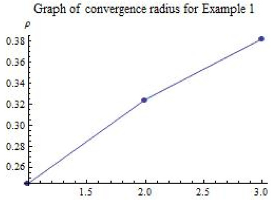
Returning to the motivational example presented in the study’s introduction, using (15) and $G^{\prime }\left({ϵ}^{*}\right)={(1,1,1)}^t$, we obtain the following.

Case ${\kappa }_0\left(u\right)=\kappa \left(u\right)=\frac{e}{2}$ provides

$${\delta }_0=0.245253.$$

Case ${\kappa }_0\left(u\right)=\frac{e-1}{2}and\kappa \left(u\right)=\frac{e}{2}$ gives

$${\delta }_1=0.324947.$$

Case ${\kappa }_0\left(u\right)=\frac{e-1}{2}and\overline{\kappa }\left(u\right)=\frac{e^{\frac{1}{(e-1)}}}{2}$ gives

$${\delta }_2=0.382692.$$

Hence, we conclude

$${\delta }_0<{\delta }_1<{\delta }_2.$$

Figure 1 also explains the advantages of different cases of κ on the convergence radius. The radius ${\delta }_0$ was given independently by Rheinboldt [1] and Traub [16], whereas radii ${\delta }_1$ and ${\delta }_2$ were reported by Argyros [3,4] for Newton’s method.

Figure 1. Convergence radius for different cases of $\kappa \left(u\right)$.

Example 2.

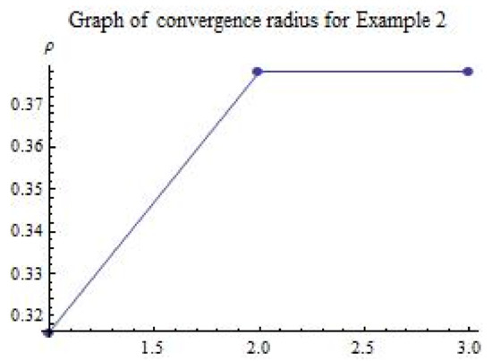
Assuming $\Re =\overline{V}(0,1)$ and ${ϵ}^{*}=0$, $\chi =Y=C[0,1]$, we describe M on ℜ such as

$$M\left(v\right)\left(x\right)=v\left(x\right)-{\int }_0^{1}x\lambda v{\left(\lambda \right)}^{3}d\lambda .$$

So,

$$M^{\prime }\left(v\left(p\right)\right)\left(x\right)=p\left(x\right)-3{\int }_0^{1}x\lambda v{\left(\lambda \right)}^{2}p\left(\lambda \right)d\lambda forallp\in \Re .$$

Then, we obtain

$${\kappa }_0\left(u\right)=1.5u<\kappa \left(u\right)=\overline{\kappa }\left(u\right)=3u.$$

As a result, by solving (15), we obtain the same advantages as in Example 1.

Old case $\kappa \left(u\right)={\kappa }_0\left(u\right)=3u$ gives

$${\delta }_0=0.316228.$$

Case $\kappa \left(u\right)=3uand{\kappa }_0\left(u\right)=1.5u$ gives

$${\delta }_1=0.377964.$$

Case $\overline{\kappa }\left(u\right)=3uand{\kappa }_0\left(u\right)=1.5u$ gives

$${\delta }_2=0.377964.$$

Hence, we conclude

$${\delta }_0<{\delta }_1\le {\delta }_2.$$

This can also be explained by Figure 2, which extends the applicability of the method through different cases of $\kappa \left(u\right)$.

Figure 2. Convergence radius for different cases of $\kappa$.

Example 3

([10]). Assume $\chi =Y=\Re$. We describe

$$G\left(u\right)={\int }_0^u\left(1+2usin\frac{\pi }{u}\right)du,\forall u\in (-\infty ,\infty ).$$

Therefore,

$$G^{\prime }\left(u\right)=\left\{\begin{array}{cc}1+2usin\frac{\pi }{u},\hfill & u\ne 0,\hfill \\ 1,\hfill & u=0,\hfill \end{array}\right..$$

Evidently, ${ϵ}^{*}=0$, $G\left(u\right)=0$, and with the help of the assumption on $G^{\prime }$

$$\left|\right|{\left[G^{\prime }\left({ϵ}^{*}\right)\right]}^{-1}(G^{\prime }\left(u\right)-G^{\prime }\left({ϵ}^{*}\right))\left|\right|=\left|2usin\frac{\pi }{u}\right|\le 2|u-{ϵ}^{*}|,\forall u\in R.$$

Theorem 4 demonstrates this for any $u_0\in \Re ({ϵ}^{*},1/6)$,

$$\left|\right|u_t-{ϵ}^{*}\left|\right|\le E^{5^t-1}\left|\right|u_0-{ϵ}^{*}\left|\right|,t=1,2,\cdots ,E=\left(\frac{16|u_0{|}^4\left[2\right|u_0|+2|y_0\left|\right]}{[1-2|u_0{\left|\right]}^3|y_0\left|\right|z_0|}\right).$$

Moreover, no other P.I.F. κ satisfies the expression (7). Observe, for example,

$$\left|\right|{\left[G^{\prime }\left({ϵ}^{*}\right)\right]}^{-1}(G^{\prime }\left(u\right)-G^{\prime }\left(y^{\lambda }\right))\left|\right|=\left|2usin\frac{\pi }{u}-2y\lambda sin\frac{\pi }{y\lambda }\right|=\frac{4}{2i+1},$$

where $u=1/i,y=1/i,\lambda =\frac{2i}{2i+1}$, and $i=1,2,\cdots$ Thus, if there exists a P.I.F. κ, i.e., relation (7) belongs in $\Re ({ϵ}^{*},\delta )$ with some $\delta >0$, as a result, there exists some $n_0>1$, i.e.,

$${\int }_0^{2r\delta }\kappa \left(u\right)du\ge \sum _{i=n_0}^{+\infty }{\int }_{\frac{4}{2i+1}}^{\frac{2}{i}}\kappa \left(u\right)du\ge \sum _{i=n_0}^{+\infty }\frac{4}{2i+1}=+\infty ,$$

which is counterintuitive. This example demonstrates that Theorem 4 is a major extension of Theorem 3, when the radius is neglected.

7. Conclusions

A novel technique was developed in order to provide a finer ball convergence analysis without making additional assumptions than in earlier studies. The method is quite generic. It turns out that while the criteria are more generic, they are also more flexible, which results in some benefits with no more computational cost. As a result, we are able to expand the usage of classified NTS to situations not previously covered. The methodology opens the door for future studies to be more effective in NTS’s convergence and other iterative procedures [9,10,11,13,14,15,19,20,21,23,25,26,27,28,29] along the same lines.

References

- Ortega, J.M.; Rheinboldt, W.C. Iterative Solution of Nonlinear Equations in Several Variables; Society for Industrial and Applied Mathematics: Philadelphia, PA, USA, 2000. [Google Scholar]
- Kantorovich, L.V.; Akilov, G.P. Functional Analysis; Pergamon Press: Oxford, UK, 1982. [Google Scholar]
- Argyros, I.K. The Theory and Applications of Iteration Methods, 2nd ed.; Engineering Series CRC Press: Boca Raton, FL, USA, 2022. [Google Scholar]
- Argyros, I.K.; Magreñán, Á.A. Iterative Methods and Their Dynamics with Applications: A Contemporary Study; CRC Press: Boca Raton, FL, USA, 2017. [Google Scholar]
- Ezquerro, J.A.; Gutiérrez, J.M.; Hernández, M.A.; Romero, N.; Rubio, M.J. The Newton Method: From Newton to Kantorovich. Gac. R. Soc. Mat. Esp. 2010, 13, 53–76. (In Spanish) [Google Scholar]
- Ezquerro, J.A.; Hernandez, M.A. Newton’s Scheme: An Updated Approach of Kantorovich’s Theory; Springer: Cham, Switzerland, 2018. [Google Scholar]
- Proinov, P.D. General local convergence theory for a class of iterative processes and its applications to Newton’s method. J. Complex. 2009, 25, 38–62. [Google Scholar] [CrossRef]
- Rall, L.B. Computational Solution of Nonlinear Operator Equations; Robert, E., Ed.; Krieger Publishing Company: New York, NY, USA, 1979. [Google Scholar]
- Ren, H.; Argyros, I.K. On the complexity of extending the convergence ball of Wang’s method for finding a zero of a derivative. J. Complex. 2021, 64, 101526. [Google Scholar] [CrossRef]
- Saxena, A.; Argyros, I.K.; Jaiswal, J.P.; Argyros, C.; Pardasani, K.R. On the Local convergence of two-step Newton type Method in Banach Spaces under generalized Lipschitz Conditions. Mathematics 2021, 9, 669. [Google Scholar] [CrossRef]
- Verma, R.U. New Trends in Fractional Programming; Nova Science Publishers: New York, NY, USA, 2019. [Google Scholar]
- Wang, X. Convergence of Newton’s method and uniqueness of the solution of equations in Banach space. IMA J. Numer. Anal. 2000, 20, 123–134. [Google Scholar] [CrossRef]
- Homeier, H.H.H. On Newton-type methods with cubic convergence. J. Comput. Appl. Math. 2005, 176, 425–432. [Google Scholar] [CrossRef]
- Kou, J.; Li, Y.; Wang, X. A modification of Newton method with third-order convergence. Appl. Math. Comput. 2006, 181, 1106–1111. [Google Scholar] [CrossRef]
- Nazeer, W.; Tanveer, M.; Kang, S.M.; Naseem, A. A new Householder’s method free from second derivatives for solving nonlinear equations and polynomiography. J. Nonlinear Sci. Appl. 2016, 9, 998–1007. [Google Scholar] [CrossRef]
- Traub, J.F. Iterative Methods for the Solution of Equations; Chelsea Publishing Company: New York, NY, USA, 1977. [Google Scholar]
- Zhanlav, T.; Chuluunbaatar, O.; Ankhbayar, G. On Newton-type methods with fourth and fifth-order convergence. Discret. Contin. Model. Appl. Comput. Sci. 2010, 2, 30–35. [Google Scholar]
- Sulaiman, I.M.; Mamat, M.; Owoyemi, A.E.; Ghazali, P.L.; Rivaie, M.; Malik, M. The convergence properties of some descent conjugate gradient algorithms for optimization models. J. Math. Comput. Sci. 2021, 22, 204–215. [Google Scholar] [CrossRef]
- Chen, J.; Li, W. Convergence behaviour of inexact Newton methods under weak Lipschitz condition. J. Comput. Appl. Math. 2006, 191, 143–164. [Google Scholar] [CrossRef]
- Kanwar, V.; Kukreja, V.K.; Singh, S. On some third-order iterative methods for solving nonlinear equations. Appl. Math. Comput. 2005, 171, 272–280. [Google Scholar]
- Magreñán, Á.A.; Argyros, I. A Contemporary Study of Iterative Methods; Elsevier: Amsterdam, The Netherlands; Academic Press: New York, NY, USA, 2018. [Google Scholar]
- Sharma, D.; Parhi, S.K. On the local convergence of modified Weerakoon’s method in Banach spaces. J. Anal. 2020, 28, 867–877. [Google Scholar] [CrossRef]
- George, S.; Argyros, I.K.A.; Jidesh, P. On the local convergence of Newton-like methods with fourth and fifth–order of convergence under hypotheses only on the first Frechet derivative. Novi Sad J. Math. 2017, 47, 1–15. [Google Scholar] [CrossRef]
- Wang, X.H.; Li, C. Convergence of Newton’s method and uniqueness of the solution of equations in Banach spaces II. Acta Math. Sin. 2003, 19, 405–412. [Google Scholar] [CrossRef]
- Shakhno, S. On a two-step iterative process under generalized Lipschitz conditions for first-order divided differences. J. Math. Sci. 2010, 168, 576–584. [Google Scholar] [CrossRef]
- Cǎtinaş, E. The inexact, inexact perturbed, and quasi-Newton methods are equivalent models. Math. Comput. 2005, 74, 291–301. [Google Scholar] [CrossRef]
- Magreñán, Á.A.; Gutiérrez, J.M. Real dynamics for damped Newton’s method applied to cubic polynomials. J. Comput. Appl. Math. 2015, 275, 527–538. [Google Scholar] [CrossRef]
- Potra, F.A.; Pták, V. Non-Discrete Induction and Iterative Processes; Research Notes in Mathematics; Pitman (Advanced Publishing Program): Boston, MA, USA, 1984. [Google Scholar]
- Singh, S.; Martínez, E.; Maroju, P.; Behl, R. A study of the local convergence of a fifth order iterative method. Indian J. Pure Appl. Math. 2020, 51, 439–455. [Google Scholar] [CrossRef]
Publisher’s Note: MDPI stays neutral with regard to jurisdictional claims in published maps and institutional affiliations. |
© 2022 by the authors. Licensee MDPI, Basel, Switzerland. This article is an open access article distributed under the terms and conditions of the Creative Commons Attribution (CC BY) license (https://creativecommons.org/licenses/by/4.0/).