The Imprecision Issues of Four Powers and Eight Predictive Powers with Historical and Interim Data

Abstract

Imprecision is commonly encountered with respect to powers and predictive powers in clinical trials. In this article, we investigate the imprecision issues of four powers (Classical Power, Classical Conditional Power, Bayesian Power, and Bayesian Conditional Power) and eight predictive powers. To begin with, we derive the probabilities of Control Superior (CS), Treatment Superior (TS), and Equivocal (E) of the four powers and the eight predictive powers, and evaluate the limits of the probabilities at point 0. Moreover, we conduct extensive numerical experiments to exemplify the imprecision issues of the four powers and the eight predictive powers. In the numerical experiments, first, we compute the probabilities of CS, TS, and E for the four powers as functions of the sample size of the future data when the true treatment effect favors control, treatment, and equivocal, respectively. Second, we compute the probabilities of CS, TS, and E for the eight predictive powers as functions of the sample size of the future data under the sceptical prior and the optimistic prior, respectively. Finally, we carry out a real data example to show the prominence of the methods.

1. Introduction

As we understand, the power with extremely distinct values at different treatment effects (for example, an observed treatment effect in the interim analysis or a treatment effect under the alternative hypothesis) may cause difficulty for interpretation. However, the predictive power, which is the prior expectation of the power and averaged over the prior distribution for the unknown true treatment effect, is better than the power in giving a favorable indication of the probability that the trial will demonstrate a positive or statistically significant outcome. The predictive power has been studied intensively in the literature [1,2,3,4,5]. In addition, the predictive power is also known as assurance [6,7,8], Probability Of Success (POS) [9,10,11], Average Success Probability (ASP) [12,13], or Contemplated Average Success Probability (CASP) [14].

The predictive power is an average power with respect to some prior, that is,

$$\mathrm{predictive}\mathrm{power}={\int }_{-\infty }^{\infty }\mathrm{power}\left(\delta \right)\times \mathrm{prior}\left(\delta \right)d\delta ,$$

where $\delta$ is the true treatment effect of the early phase and Phase III trials. As described in [5], there are eight predictive powers with historical and interim data, because we have four choices for $\mathrm{power}\left(\delta \right)$, including the Classical Power (CP) which does not use any data, the Classical Conditional Power (CCP), which uses the interim data once, the Bayesian Power (BP), which uses the historical data once, and the Bayesian Conditional Power (BCP) which uses the historical data once and the interim data once; and we have two choices for $\mathrm{prior}\left(\delta \right)$, including $\pi \left(\delta |d_0\right)$ which uses the historical data once, and $\pi \left(\delta |d_0,d_1\right)$ which uses the historical data once and the interim data once, where $d_0$ are the historical data, and $d_1$ are the interim data. As described in [5], the eight predictive powers are $I_1$ which is the Classical Predictive Power (CPP), $I_2$ which is the Classical Interim Predictive Power (CIPP), $I_3$, which is the Classical Conditional Predictive Power (CCPP), $I_4$, which is the Classical Conditional Interim Predictive Power (CCIPP), $I_5$, which is the Bayesian Predictive Power (BPP), $I_6$, which is the Bayesian Interim Predictive Power (BIPP), $I_7$, which is the Bayesian Conditional Predictive Power (BCPP), and $I_8$, which is the Bayesian Conditional Interim Predictive Power (BCIPP), where I is short for integral, indicating that the predictive powers are integrals. In the literature, most researchers consider $I_1$, the CPP (see (6.4) in [15], (6) in [6], and (2) in [12]). Moreover, in [15], they also consider $I_4$ (CCIPP, (6.15) in [15]), $I_5$ (BPP, (6.7) in [15]), and $I_8$ (BCIPP, (6.18) in [15]). In this article, we are interested in the four powers (CP, CCP, BP, and BCP) and the eight predictive powers.

The imprecision issues of the four powers and the eiht predictive powers are investigated in this article. Imprecision means that $m_2$ is small, where $m_2$ is the sample size of the future data. Imprecision issue means when $m_2$ is small (imprecision), the probability of Equivocal (E) is large, and thus, it is hard to discriminate between Control Superior (CS) and Treatment Superior (TS). For the four powers, when the true treatment effect favors treatment, the probabilities of TS are increasing functions of $m_2$. Moreover, for the eight predictive powers under the optimistic prior, the probabilities of TS are also increasing functions of $m_2$. As a result, when $m_2$ is small (imprecision), the probabilities of TS or the probabilities of success will be small. Hence, it is probably that the trial will end up with a no-go decision and a prospective drug will be killed because of small $m_2$. Therefore, imprecision is an important issue that should be studied thoroughly.

In [5], under normal models of the data, they expand the four predictive powers in [15] to eight predictive powers for the hypotheses $H_0:\delta \le {\delta }_0$ versus $H_1:\delta >{\delta }_0$ and the reversed hypotheses $H_0:\delta \ge {\delta }_0$ versus $H_1:\delta <{\delta }_0$, where ${\delta }_0$ is a threshold value for $\delta$, and the results are summarized in two tables. Namely, they have discovered four predictive powers with the historical and interim data for the hypotheses and the reversed hypotheses. Moreover, the eight predictive powers are utilized to guide the futility analysis in the tamoxifen example, in which a long-term tamoxifen therapy is used to prevent the recurrence of breast cancer. The tamoxifen example is a Phase III trial and the predictive powers suggest them to stop the trial for futility. In the Conclusions and Discussion section of [5], they state that “The way the results are presented right now suggests to stop the trial for futility but this may in fact be an imprecision issue due to small $m_2$ (or limited overall number of events)…”. In this article, we will have an in-depth study on the imprecision issues of the four powers and the eight predictive powers.

The main contributions of this article are summarized as follows. We have evaluated the limits at point 0 of the probabilities of CS, TS, and E of the four powers and the eight predictive powers. Moreover, we have conducted extensive numerical experiments to exemplify the imprecision issues of the four powers and the eight predictive powers. In the numerical experiments, first, we have computed the probabilities of CS, TS, and E for the four powers as functions of $m_2$ when the true treatment effect favors control, treatment, and equivocal, respectively. Second, we have computed the probabilities of CS, TS, and E for the eight predictive powers as functions of $m_2$ under the sceptical prior and the optimistic prior, respectively. Finally, we have carried out a real data example to show the prominence of the methods.

The rest of the article is organized as follows. In Section 2, we will derive the probabilities of CS, TS, and E of the four powers and the eight predictive powers, and evaluate the limits of the probabilities at point 0. Section 3 conducts extensive numerical experiments to exemplify the imprecision issues of the four powers and the eight predictive powers. In Section 4, we will perform some numerical experiments for a real data example. Section 5 provides some conclusions and discussions.

2. The Four Powers and the Eight Predictive Powers, and Their Limits at 0

In this section, after some preliminary results, we will derive the probabilities of CS, TS, and E of the four powers and the eight predictive powers, and evaluate their limits at point 0 ($m_2\to 0^{+}$).

2.1. Preliminary

In this subsection, we will give some preliminary results.

The four powers, the eight predictive powers, and the data structures of the historical data, interim data, and future data are described in Figure 1. On the basis of Figure 1 in [5], we have added the four powers in the two plots. From Figure 1, we see that the time when CP and BP are calculated in the upper plot is at the end of early phase and before the start of Phase III. At that time, only the first and fifth predictive powers can be calculated. Moreover, the time when CCP and BCP are calculated in the lower plot is at the interim of the Phase III trial. At the interim, there are six predictive powers; that is, the second, third, fourth, sixth, seventh, and eighth predictive powers. As described in [5], in the figure, H means historical data, I means interim data, and F means future data. The historical data could be the Phase II data, or the previous Phase III data, provided that the outcome variable and patient populations are the same between the historical data and the new Phase III data. Furthermore, the historical data could also be fictitious data corresponding to a sceptical or an optimistic prior, and in this case, $d_0$ and $m_0$ of the historical data are calculated to satisfy the requirements of the sceptical or optimistic prior. Notice that $d_0$, $d_1$, and $d_2$ are the observed treatment differences in the treatment group and the control (or placebo) group means of the historical data, interim data, and future data, respectively, and $m_0$, $m_1$, and $m_2$ are the per group numbers of patients of the historical data, interim data, and future data, respectively.

Let us use the normal models given in [5]. For CP, BP, $I_1$, and $I_5$, the model and prior are given by

$$d_2|\delta \sim N\left(\delta ,\frac{2{\sigma }^2}{m_2}\right),\delta |d_0\sim N\left(d_0,\frac{2{\sigma }^2}{m_0}\right),$$

(1)

which implies

$$\begin{array}{cc}\hfill \delta |d_0,d_2& \sim N\left(\frac{m_0{d}_0+m_2{d}_2}{m_0+m_2},\frac{2{\sigma }^2}{m_0+m_2}\right),\hfill \\ \hfill d_2|d_0& \sim N\left(d_0,2{\sigma }^2\left(\frac{1}{m_0}+\frac{1}{m_2}\right)\right),\hfill \end{array}$$

where $\delta$ is the unknown true treatment effect, and ${\sigma }^2$ is a common known variance. The data structure of (1) is depicted in the upper plot of Figure 1. For CCP, BCP, $I_2$, $I_3$, $I_4$, $I_6$, $I_7$, and $I_8$, the model and prior are given by

$$d_1|\delta \sim N\left(\delta ,\frac{2{\sigma }^2}{m_1}\right),d_2|\delta \sim N\left(\delta ,\frac{2{\sigma }^2}{m_2}\right),\delta |d_0\sim N\left(d_0,\frac{2{\sigma }^2}{m_0}\right),$$

(2)

which leads to

$$\begin{array}{cc}\hfill \delta |d_0,d_1,d_2& \sim N\left(\frac{m_0{d}_0+m_1{d}_1+m_2{d}_2}{m_0+m_1+m_2},\frac{2{\sigma }^2}{m_0+m_1+m_2}\right),\hfill \\ \hfill d_2|d_0,d_1& \sim N\left(\frac{m_0{d}_0+m_1{d}_1}{m_0+m_1},2{\sigma }^2\left(\frac{1}{m_2}+\frac{1}{m_0+m_1}\right)\right).\hfill \end{array}$$

The data structure of (2) is depicted in the lower plot of Figure 1.

We will consider the hypotheses

$$H_0:\delta \le 0\mathrm{versus}{H}_1:\delta >0.$$

(3)

This kind of hypothesis arises when we assume that a larger value in the population mean of the normal distribution means improvement in disease condition. Hence, a positive value of $\delta$ means better. Moreover, we are also interested in the reversed hypotheses

$$H_0:\delta \ge 0\mathrm{versus}{H}_1:\delta <0.$$

(4)

This kind of hypothesis arises when we assume that a smaller value in the population mean of the normal distribution means improvement in disease condition. Hence, a negative value of $\delta$ means a better condition.

There are three conclusions, namely, CS, TS, and E. In terms of the $\delta$ values, assume that

$$\begin{array}{cc}\hfill {\mathrm{CS}}_{\mathrm{TC}}& \iff \delta >0,\hfill \\ \hfill {\mathrm{TS}}_{\mathrm{TC}}& \iff \delta <0,\hfill \\ \hfill {\mathrm{E}}_{\mathrm{TC}}& \iff \delta =0,\hfill \end{array}$$

where $\mathrm{TC}$ stands for True Condition. For example, let $h_1$ and $h_2$ be the hazard rates corresponding to treatment and control, respectively. Hence,

$$\begin{array}{cc}\hfill {\mathrm{CS}}_{\mathrm{TC}}& \iff h_1>h_2\iff HR=\frac{h_1}{h_2}>1\iff \delta =log\left(HR\right)>0,\hfill \\ \hfill {\mathrm{TS}}_{\mathrm{TC}}& \iff h_1<h_2\iff HR=\frac{h_1}{h_2}<1\iff \delta =log\left(HR\right)<0,\hfill \\ \hfill {\mathrm{E}}_{\mathrm{TC}}& \iff h_1=h_2\iff HR=\frac{h_1}{h_2}=1\iff \delta =log\left(HR\right)=0,\hfill \end{array}$$

where $HR$ is the Hazard Ratio. In terms of confidence or credible intervals of $\delta$, we have

$$\begin{array}{cc}\hfill {\mathrm{CS}}_{\mathrm{D}}& \iff \mathrm{the}1-\alpha \mathrm{confidence}\mathrm{or}\mathrm{credible}\mathrm{interval}\mathrm{of}\delta \mathrm{with}\mathrm{lower}\mathrm{limit}[L,\infty )\mathrm{lying}\mathrm{wholly}\mathrm{above}0,\hfill \\ \hfill {\mathrm{TS}}_{\mathrm{D}}& \iff \mathrm{the}1-\alpha \mathrm{confidence}\mathrm{or}\mathrm{credible}\mathrm{interval}\mathrm{of}\delta \mathrm{with}\mathrm{upper}\mathrm{limit}(-\infty ,U]\mathrm{lying}\mathrm{wholly}\mathrm{below}0,\hfill \\ \hfill {\mathrm{E}}_{\mathrm{D}}& \iff \mathrm{the}1-2\alpha \mathrm{confidence}\mathrm{or}\mathrm{credible}\mathrm{interval}\mathrm{of}\delta \mathrm{with}\mathrm{lower}\mathrm{and}\mathrm{upper}\mathrm{limits}[L,U]\mathrm{including}0,\hfill \end{array}$$

where $\mathrm{D}$ stands for Decision.

2.2. The CP, and the First and Second Predictive Powers

In this subsection, we will calculate the confidence intervals of $\delta$ with lower, upper, and both limits for the Classical Power (CP). Moreover, we will derive the probabilities of CS, TS, and E of the CP and the first and second predictive powers, and evaluate their limits at point 0.

Let us first calculate the confidence intervals of $\delta$ with lower, upper, and both limits for the CP. The CP is the probability of the classical rejection region with $d_2$,

$$S_{\alpha ,0}^{C,d_2}=\left\{d_2>Z_{\alpha }\sigma \sqrt{2/m_2}\right\},$$

given a value for $\delta$, that is, $\mathrm{CP}=P\left(S_{\alpha ,0}^{C,d_2}|\delta \right)$. It is easy to show that the $1-\alpha$ confidence interval of $\delta$ with lower limit for the CP is

$$[d_2-Z_{\alpha }\sigma \sqrt{2/m_2},\infty ).$$

Now, let us consider the ${\mathrm{CP}}^{-}$, which is the probability of the classical rejection region with $d_2$,

$$S_{\alpha ,0}^{C-,d_2}=\left\{d_2<-Z_{\alpha }\sigma \sqrt{2/m_2}\right\},$$

given a value for $\delta$, that is, ${\mathrm{CP}}^{-}=P\left(S_{\alpha ,0}^{C-,d_2}|\delta \right)$. It is easy to show that the $1-\alpha$ confidence interval of $\delta$ with upper limit for the CP is

$$(-\infty ,d_2+Z_{\alpha }\sigma \sqrt{2/m_2}].$$

Moreover, the $1-2\alpha$ confidence interval of $\delta$ with lower and upper limits for the CP is

$$\left[d_2-Z_{\alpha }\sigma \sqrt{2/m_2},d_2+Z_{\alpha }\sigma \sqrt{2/m_2}\right].$$

(5)

It is worth noting that the confidence level related to the lower or upper limit for the CP is $1-\alpha$, while the confidence level related to both limits for the CP is $1-2\alpha$.

The expressions of the probabilities $P\left(\mathrm{CS}:\mathrm{CP}\right)$, $P\left(\mathrm{TS}:\mathrm{CP}\right)$, $P\left(\mathrm{E}:\mathrm{CP}\right)$, $P\left(\mathrm{CS}:I_1\right)$, $P\left(\mathrm{TS}:I_1\right)$, $P\left(\mathrm{E}:I_1\right)$, $P\left(\mathrm{CS}:I_2\right)$, $P\left(\mathrm{TS}:I_2\right)$, and $P\left(\mathrm{E}:I_2\right)$ are given in Supplementary Materials. Note that the CS, TS, and E in the probabilities are for decisions. However, the subscripts $\mathrm{D}$ are omitted to lighten notations.

The main theoretical contributions of this article are summarized in the following four propositions, whose proofs are given in Supplementary Materials.

The limits at point 0 of the probabilities of CS, TS, and E of the CP and the first and second predictive powers are summarized in the following proposition.

Proposition 1.

The limits at point 0 of the probabilities of CS, TS, and E of the CP and the first and second predictive powers are given by

$$\begin{array}{cc}\hfill \underset{m_2\to 0^{+}}{lim}P\left(CS:CP\right)& =\underset{m_2\to 0^{+}}{lim}P\left(CS:I_1\right)=\underset{m_2\to 0^{+}}{lim}P\left(CS:I_2\right)=\alpha ,\hfill \\ \hfill \underset{m_2\to 0^{+}}{lim}P\left(TS:CP\right)& =\underset{m_2\to 0^{+}}{lim}P\left(TS:I_1\right)=\underset{m_2\to 0^{+}}{lim}P\left(TS:I_2\right)=\alpha ,\hfill \\ \hfill \underset{m_2\to 0^{+}}{lim}P\left(E:CP\right)& =\underset{m_2\to 0^{+}}{lim}P\left(E:I_1\right)=\underset{m_2\to 0^{+}}{lim}P\left(E:I_2\right)=1-2\alpha .\hfill \end{array}$$

(6)

Therefore, when $m_2$ is small (imprecision), the probabilities $P\left(\mathrm{E}:\mathrm{CP}\right)$, $P\left(\mathrm{E}:I_1\right)$, and $P\left(\mathrm{E}:I_2\right)$ are large.

2.3. The CCP, and the Third and Fourth Predictive Powers

In this subsection, we will calculate the confidence intervals of $\delta$ with lower, upper, and both limits for the Classical Conditional Power (CCP). Moreover, we will derive the probabilities of CS, TS, and E of the CCP and the third and fourth predictive powers, and evaluate their limits at point 0.

Let us first calculate the confidence intervals of $\delta$ with lower, upper, and both limits for the CCP. The CCP is the probability of the classical rejection region with $d_1$ and $d_2$,

$$S_{\alpha ,0}^{C,d_1,d_2}=\left\{d_2>\frac{Z_{\alpha }\sigma \sqrt{2\left(m_1+m_2\right)}-m_1{d}_1}{m_2}\right\},$$

given values of $\delta$ and the interim result $d_1$, that is, $\mathrm{CCP}=P\left(S_{\alpha ,0}^{C,d_1,d_2}|\delta ,d_1\right)$. It is easy to show that the $1-\alpha$ confidence interval of $\delta$ with a lower limit for the CCP is

$$\left[\frac{m_1{d}_1+m_2{d}_2}{m_1+m_2}-Z_{\alpha }\sigma \sqrt{\frac{2}{m_1+m_2}},\infty \right).$$

Now let us consider the ${\mathrm{CCP}}^{-}$, which is the probability of the classical rejection region with $d_1$ and $d_2$,

$$S_{\alpha ,0}^{C-,d_1,d_2}=\left\{d_2<\frac{-Z_{\alpha }\sigma \sqrt{2\left(m_1+m_2\right)}-m_1{d}_1}{m_2}\right\},$$

given values of $\delta$ and the interim result $d_1$, that is, ${\mathrm{CCP}}^{-}=P\left(S_{\alpha ,0}^{C-,d_1,d_2}|\delta ,d_1\right)$. It is easy to show that the $1-\alpha$ confidence interval of $\delta$ with the upper limit for the CCP is

$$\left(-\infty ,\frac{m_1{d}_1+m_2{d}_2}{m_1+m_2}+Z_{\alpha }\sigma \sqrt{\frac{2}{m_1+m_2}}\right].$$

Moreover, the $1-2\alpha$ confidence interval of $\delta$ with lower and upper limits for the CCP is

$$\left[\frac{m_1{d}_1+m_2{d}_2}{m_1+m_2}-Z_{\alpha }\sigma \sqrt{\frac{2}{m_1+m_2}},\frac{m_1{d}_1+m_2{d}_2}{m_1+m_2}+Z_{\alpha }\sigma \sqrt{\frac{2}{m_1+m_2}}\right].$$

(7)

It is worth noting that the confidence level related to the lower or upper limit for the CCP is $1-\alpha$, while the confidence level related to both limits for the CCP is $1-2\alpha$.

The expressions of the probabilities $P\left(\mathrm{CS}:\mathrm{CCP}\right)$, $P\left(\mathrm{TS}:\mathrm{CCP}\right)$, $P\left(\mathrm{E}:\mathrm{CCP}\right)$, $P\left(\mathrm{CS}:I_3\right)$, $P\left(\mathrm{TS}:I_3\right)$, $P\left(\mathrm{E}:I_3\right)$, $P\left(\mathrm{CS}:I_4\right)$, $P\left(\mathrm{TS}:I_4\right)$, and $P\left(\mathrm{E}:I_4\right)$ are given in Supplementary Materials. For clinical trials with interim data, we have

$$m_1+m_2=s,$$

and thus,

$$m_1\to s\mathrm{as}{m}_2\to 0^{+},$$

where s is the subtotal sample size of the early trial and the confirmatory trial of one arm.

The limits at point 0 of the probabilities of CS, TS, and E of the CCP and the third and fourth predictive powers are summarized in the following proposition.

Proposition 2.

The limits at point 0 of the probabilities of CS, TS, and E of the CCP and the third and fourth predictive powers are given by

$$\begin{array}{cc}\hfill & \underset{m_2\to 0^{+}}{lim}P\left(CS:CCP\right)\underset{m_2\to 0^{+}}{=lim}P\left(CS:I_3\right)=\underset{m_2\to 0^{+}}{lim}P\left(CS:I_4\right)\hfill \\ \hfill & =\left\{\begin{array}{cc}1,\hfill & \mathrm{if}{d}_1>Z_{\alpha }\sigma \sqrt{2/s},\hfill \\ 0.5,\hfill & \mathrm{if}{d}_1=Z_{\alpha }\sigma \sqrt{2/s},\hfill \\ 0,\hfill & \mathrm{if}{d}_1<Z_{\alpha }\sigma \sqrt{2/s},\hfill \end{array}\right.\hfill \end{array}$$

(8)

$$\begin{array}{cc}\hfill & \underset{m_2\to 0^{+}}{lim}P\left(TS:CCP\right)\underset{m_2\to 0^{+}}{=lim}P\left(TS:I_3\right)=\underset{m_2\to 0^{+}}{lim}P\left(TS:I_4\right)\hfill \\ \hfill & =\left\{\begin{array}{cc}1,\hfill & \mathrm{if}{d}_1<-Z_{\alpha }\sigma \sqrt{2/s},\hfill \\ 0.5,\hfill & \mathrm{if}{d}_1=-Z_{\alpha }\sigma \sqrt{2/s},\hfill \\ 0,\hfill & \mathrm{if}{d}_1>-Z_{\alpha }\sigma \sqrt{2/s},\hfill \end{array}\right.\hfill \end{array}$$

(9)

and

$$\begin{array}{cc}\hfill & \underset{m_2\to 0^{+}}{lim}P\left(E:CCP\right)\underset{m_2\to 0^{+}}{=lim}P\left(E:I_3\right)=\underset{m_2\to 0^{+}}{lim}P\left(E:I_4\right)\hfill \\ \hfill & =\left\{\begin{array}{cc}0,\hfill & \mathrm{if}{d}_1<-Z_{\alpha }\sigma \sqrt{2/s},\hfill \\ 0.5,\hfill & \mathrm{if}{d}_1=-Z_{\alpha }\sigma \sqrt{2/s},\hfill \\ 1,\hfill & \mathrm{if}-Z_{\alpha }\sigma \sqrt{2/s}<d_1<Z_{\alpha }\sigma \sqrt{2/s},\hfill \\ 0.5,\hfill & \mathrm{if}{d}_1=Z_{\alpha }\sigma \sqrt{2/s},\hfill \\ 0,\hfill & \mathrm{if}{d}_1>Z_{\alpha }\sigma \sqrt{2/s}.\hfill \end{array}\right.\hfill \end{array}$$

(10)

The graph of the three limits (8)–(10) by one plot is depicted in Web Figure S1.

Alternatively, the graph of the three limits (8)–(10) by three plots is depicted in Figure 2.

2.4. The BP, and the Fifth and Sixth Predictive Powers

In this subsection, we will calculate the credible intervals of $\delta$ with lower, upper, and both limits for the Bayesian Power (BP). Moreover, we will derive the probabilities of CS, TS, and E of the BP and the fifth and sixth predictive powers, and evaluate their limits at point 0.

Let us first calculate the credible intervals of $\delta$ with lower, upper, and both limits for the BP. The BP is the probability of the Bayesian rejection region with $d_0,d_2$,

$$S_{\alpha ,0}^{B,d_0,d_2}=\left\{d_2>\frac{Z_{\alpha }\sigma \sqrt{2\left(m_0+m_2\right)}-m_0{d}_0}{m_2}\right\},$$

given values of $\delta$ and the historical result $d_0$, that is, $\mathrm{BP}=P\left(S_{\alpha ,0}^{B,d_0,d_2}|\delta ,d_0\right)$. It is easy to show that the $1-\alpha$ credible interval of $\delta$ with a lower limit for the BP is

$$\left[\frac{m_0{d}_0+m_2{d}_2}{m_0+m_2}-Z_{\alpha }\sigma \sqrt{\frac{2}{m_0+m_2}},\infty \right).$$

Now, let us consider the ${\mathrm{BP}}^{-}$, which is the probability of the Bayesian rejection region with $d_0,d_2$,

$$S_{\alpha ,0}^{B-,d_0,d_2}=\left\{d_2<\frac{-Z_{\alpha }\sigma \sqrt{2\left(m_0+m_2\right)}-m_0{d}_0}{m_2}\right\},$$

given values of $\delta$ and historical result $d_0$, that is, ${\mathrm{BP}}^{-}=P\left(S_{\alpha ,0}^{B-,d_0,d_2}|\delta ,d_0\right)$. It is easy to show that the $1-\alpha$ credible interval of $\delta$ with an upper limit for the BP is

$$\left(-\infty ,\frac{m_0{d}_0+m_2{d}_2}{m_0+m_2}+Z_{\alpha }\sigma \sqrt{\frac{2}{m_0+m_2}}\right].$$

Moreover, the $1-2\alpha$ credible interval of $\delta$ with lower and upper limits for the BP is

$$\left[\frac{m_0{d}_0+m_2{d}_2}{m_0+m_2}-Z_{\alpha }\sigma \sqrt{\frac{2}{m_0+m_2}},\frac{m_0{d}_0+m_2{d}_2}{m_0+m_2}+Z_{\alpha }\sigma \sqrt{\frac{2}{m_0+m_2}}\right].$$

(11)

It is worth noting that the credible level related to the lower or upper limit for the BP is $1-\alpha$, while the credible level related to both limits for the BP is $1-2\alpha$.

The expressions of the probabilities $P\left(\mathrm{CS}:\mathrm{BP}\right)$, $P\left(\mathrm{TS}:\mathrm{BP}\right)$, $P\left(\mathrm{E}:\mathrm{BP}\right)$, $P\left(\mathrm{CS}:I_5\right)$, $P\left(\mathrm{TS}:I_5\right)$, $P\left(\mathrm{E}:I_5\right)$, $P\left(\mathrm{CS}:I_6\right)$, $P\left(\mathrm{TS}:I_6\right)$, and $P\left(\mathrm{E}:I_6\right)$ are given in Supplementary Materials.

The limits at point 0 of the probabilities of CS, TS, and E of the BP and the fifth and sixth predictive powers are summarized in the following proposition.

Proposition 3.

The limits at point 0 of the probabilities of CS, TS, and E of the BP and the fifth and sixth predictive powers are given by

$$\begin{array}{cc}\hfill & \underset{m_2\to 0^{+}}{lim}P\left(CS:BP\right)\underset{m_2\to 0^{+}}{=lim}P\left(CS:I_5\right)=\underset{m_2\to 0^{+}}{lim}P\left(CS:I_6\right)\hfill \\ \hfill & =\left\{\begin{array}{cc}1,\hfill & \mathrm{if}{d}_0>Z_{\alpha }\sigma \sqrt{2/m_0},\hfill \\ 0.5,\hfill & \mathrm{if}{d}_0=Z_{\alpha }\sigma \sqrt{2/m_0},\hfill \\ 0,\hfill & \mathrm{if}{d}_0<Z_{\alpha }\sigma \sqrt{2/m_0},\hfill \end{array}\right.\hfill \end{array}$$

(12)

$$\begin{array}{cc}\hfill & \underset{m_2\to 0^{+}}{lim}P\left(TS:BP\right)\underset{m_2\to 0^{+}}{=lim}P\left(TS:I_5\right)=\underset{m_2\to 0^{+}}{lim}P\left(TS:I_6\right)\hfill \\ \hfill & =\left\{\begin{array}{cc}1,\hfill & \mathrm{if}{d}_0<-Z_{\alpha }\sigma \sqrt{2/m_0},\hfill \\ 0.5,\hfill & \mathrm{if}{d}_0=-Z_{\alpha }\sigma \sqrt{2/m_0},\hfill \\ 0,\hfill & \mathrm{if}{d}_0>-Z_{\alpha }\sigma \sqrt{2/m_0},\hfill \end{array}\right.\hfill \end{array}$$

(13)

and

$$\begin{array}{cc}\hfill & \underset{m_2\to 0^{+}}{lim}P\left(E:BP\right)\underset{m_2\to 0^{+}}{=lim}P\left(E:I_5\right)=\underset{m_2\to 0^{+}}{lim}P\left(E:I_6\right)\hfill \\ \hfill & =\left\{\begin{array}{cc}0,\hfill & \mathrm{if}{d}_0<-Z_{\alpha }\sigma \sqrt{2/m_0},\hfill \\ 0.5,\hfill & \mathrm{if}{d}_0=-Z_{\alpha }\sigma \sqrt{2/m_0},\hfill \\ 1,\hfill & \mathrm{if}-Z_{\alpha }\sigma \sqrt{2/m_0}<d_0<Z_{\alpha }\sigma \sqrt{2/m_0},\hfill \\ 0.5,\hfill & \mathrm{if}{d}_0=Z_{\alpha }\sigma \sqrt{2/m_0},\hfill \\ 0,\hfill & \mathrm{if}{d}_0>Z_{\alpha }\sigma \sqrt{2/m_0}.\hfill \end{array}\right.\hfill \end{array}$$

(14)

2.5. The BCP, and the Seventh and Eighth Predictive Powers

In this subsection, we will calculate the credible intervals of $\delta$ with lower, upper, and both limits for the Bayesian Conditional Power (BCP). Moreover, we will derive the probabilities of CS, TS, and E of the BCP and the seventh and eighth predictive powers, and evaluate their limits at point 0.

Let us first calculate the credible intervals of $\delta$ with lower, upper, and both limits for the BCP. The BCP is the probability of the Bayesian rejection region with $d_0,d_1,d_2$,

$$S_{\alpha ,0}^{B,d_0,d_1,d_2}=\left\{d_2>\frac{Z_{\alpha }\sigma \sqrt{2\left(m_0+m_1+m_2\right)}-m_0{d}_0-m_1{d}_1}{m_2}\right\},$$

given values of $\delta ,d_0,d_1$, that is, $\mathrm{BCP}=P\left(S_{\alpha ,0}^{B,d_0,d_1,d_2}|\delta ,d_0,d_1\right)$. It is easy to show that the $1-\alpha$ credible interval of $\delta$ with lower limit for the BCP is

$$\left[\frac{m_0{d}_0+m_1{d}_1+m_2{d}_2}{m_0+m_1+m_2}-Z_{\alpha }\sigma \sqrt{\frac{2}{m_0+m_1+m_2}},\infty \right).$$

Now, let us consider the ${\mathrm{BCP}}^{-}$, which is the probability of the Bayesian rejection region with $d_0,d_1,d_2$,

$$S_{\alpha ,0}^{B-,d_0,d_1,d_2}=\left\{d_2<\frac{-Z_{\alpha }\sigma \sqrt{2\left(m_0+m_1+m_2\right)}-m_0{d}_0-m_1{d}_1}{m_2}\right\},$$

given values of $\delta ,d_0,d_1$, that is, ${\mathrm{BCP}}^{-}=P\left(S_{\alpha ,0}^{B-,d_0,d_1,d_2}|\delta ,d_0,d_1\right)$. It is easy to show that the $1-\alpha$ credible interval of $\delta$ with the upper limit for the BCP is

$$\left(-\infty ,\frac{m_0{d}_0+m_1{d}_1+m_2{d}_2}{m_0+m_1+m_2}+Z_{\alpha }\sigma \sqrt{\frac{2}{m_0+m_1+m_2}}\right].$$

Moreover, the $1-2\alpha$ credible interval of $\delta$ with lower and upper limits for the BCP is

$$\left[\frac{m_0{d}_0+m_1{d}_1+m_2{d}_2}{m_0+m_1+m_2}-Z_{\alpha }\sigma \sqrt{\frac{2}{m_0+m_1+m_2}},\frac{m_0{d}_0+m_1{d}_1+m_2{d}_2}{m_0+m_1+m_2}+Z_{\alpha }\sigma \sqrt{\frac{2}{m_0+m_1+m_2}}\right].$$

(15)

It is worth noting that the credible level related to the lower or upper limit for the BCP is $1-\alpha$, while the credible level related to both limits for the BCP is $1-2\alpha$.

The expressions of the probabilities $P\left(\mathrm{CS}:\mathrm{BCP}\right)$, $P\left(\mathrm{TS}:\mathrm{BCP}\right)$, $P\left(\mathrm{E}:\mathrm{BCP}\right)$, $P\left(\mathrm{CS}:I_7\right)$, $P\left(\mathrm{TS}:I_7\right)$, $P\left(\mathrm{E}:I_7\right)$, $P\left(\mathrm{CS}:I_8\right)$, $P\left(\mathrm{TS}:I_8\right)$, and $P\left(\mathrm{E}:I_8\right)$ are given in Supplementary Materials.

The limits at point 0 of the probabilities of CS, TS, and E of the BCP and the seventh and eighth predictive powers are summarized in the following proposition.

Proposition 4.

The limits at point 0 of the probabilities of CS, TS, and E of the BCP and the seventh and eighth predictive powers are given by

$$\begin{array}{cc}\hfill & \underset{m_2\to 0^{+}}{lim}P\left(CS:BCP\right)=\underset{m_2\to 0^{+}}{lim}P\left(CS:I_7\right)=\underset{m_2\to 0^{+}}{lim}P\left(CS:I_8\right)\hfill \\ \hfill & =\left\{\begin{array}{cc}1,\hfill & \mathrm{if}{m}_0{d}_0+s{d}_1>Z_{\alpha }\sigma \sqrt{2\left(m_0+s\right)},\hfill \\ 0.5,\hfill & \mathrm{if}{m}_0{d}_0+s{d}_1=Z_{\alpha }\sigma \sqrt{2\left(m_0+s\right)},\hfill \\ 0,\hfill & \mathrm{if}{m}_0{d}_0+s{d}_1<Z_{\alpha }\sigma \sqrt{2\left(m_0+s\right)},\hfill \end{array}\right.\hfill \end{array}$$

(16)

$$\begin{array}{cc}\hfill & \underset{m_2\to 0^{+}}{lim}P\left(TS:BCP\right)=\underset{m_2\to 0^{+}}{lim}P\left(TS:I_7\right)=\underset{m_2\to 0^{+}}{lim}P\left(TS:I_8\right)\hfill \\ \hfill & =\left\{\begin{array}{cc}1,\hfill & \mathrm{if}{m}_0{d}_0+s{d}_1<-Z_{\alpha }\sigma \sqrt{2\left(m_0+s\right)},\hfill \\ 0.5,\hfill & \mathrm{if}{m}_0{d}_0+s{d}_1=-Z_{\alpha }\sigma \sqrt{2\left(m_0+s\right)},\hfill \\ 0,\hfill & \mathrm{if}{m}_0{d}_0+s{d}_1>-Z_{\alpha }\sigma \sqrt{2\left(m_0+s\right)},\hfill \end{array}\right.\hfill \end{array}$$

(17)

and

$$\begin{array}{cc}\hfill & \underset{m_2\to 0^{+}}{lim}P\left(E:BCP\right)=\underset{m_2\to 0^{+}}{lim}P\left(E:I_7\right)=\underset{m_2\to 0^{+}}{lim}P\left(E:I_8\right)\hfill \\ \hfill & =\left\{\begin{array}{cc}0,\hfill & \mathrm{if}{m}_0{d}_0+s{d}_1<-Z_{\alpha }\sigma \sqrt{2\left(m_0+s\right)},\hfill \\ 0.5,\hfill & \mathrm{if}{m}_0{d}_0+s{d}_1=-Z_{\alpha }\sigma \sqrt{2\left(m_0+s\right)},\hfill \\ 1,\hfill & \mathrm{if}-Z_{\alpha }\sigma \sqrt{2\left(m_0+s\right)}<m_0{d}_0+s{d}_1<Z_{\alpha }\sigma \sqrt{2\left(m_0+s\right)},\hfill \\ 0.5,\hfill & \mathrm{if}{m}_0{d}_0+s{d}_1=Z_{\alpha }\sigma \sqrt{2\left(m_0+s\right)},\hfill \\ 0,\hfill & \mathrm{if}{m}_0{d}_0+s{d}_1>Z_{\alpha }\sigma \sqrt{2\left(m_0+s\right)}.\hfill \end{array}\right.\hfill \end{array}$$

(18)

3. Numerical Experiments

In this section, we will conduct extensive numerical experiments to exemplify the imprecision issues of the four powers and the eight predictive powers. First, we will compute the probabilities of CS, TS, and E for the four powers as functions of $m_2$ when $\delta =1$, which favors control, $\delta =-1$, which favors treatment, and $\delta =0$, which favors equivocal, respectively. Second, we will compute the probabilities of CS, TS, and E for the eight predictive powers as functions of $m_2$ under the sceptical prior and the optimistic prior, respectively.

As was used in [5,15], we assume that

$$\begin{array}{cc}\hfill \alpha & =0.025,\sigma =\sqrt{2},{\mu }_s=0,{\mu }_o=log\left(0.6\right)\approx -0.51,\hfill \\ \hfill m_0^r& \approx 41.4,m_1^r=46,m_2^r\left\{\begin{array}{cc}=s=115,\hfill & \mathrm{for}i=1,5,\hfill \\ =s-m_1^r=69,\hfill & \mathrm{for}i=2,3,4,6,7,8,\hfill \end{array}\right.\hfill \\ \hfill d_1^r& =0.435,s=115,t^r=\frac{m_1^r}{s}=0.4,\hfill \end{array}$$

(19)

where

$$m_0^r={\left(\frac{{\mathrm{\Phi }}^{-1}\left(0.05\right)\sqrt{2}\sigma }{{\mu }_o}\right)}^2\approx 41.4,$$

is calculated to ensure that an optimistic prior was centered on a $40\%$ hazard reduction and a $5\%$ chance of a negative effect (i.e., $HR>1$), equivalent on the $log\left(HR\right)$ scale to a normal prior with mean ${\mu }_o=log\left(0.6\right)\approx -0.51$ and standard deviation $0.31$ ($\sigma =\sqrt{2}$, $m_0^r\approx 41.4$). The sceptical prior was adopted as a normal distribution with the same standard deviation as the optimistic prior, but centered on ${\mu }_s=0$. The superscripts “r” in $m_0^r$, $m_1^r$, $m_2^r$, $d_1^r$, and $t^r$ are added to indicate that they are from the real data.

The four powers and the eight predictive powers as functions of the parameters and the data used are summarized in

Table 1. The 4 powers and the 8 predictive powers as functions of the parameters, and the data used.

	$\mathit{\alpha }$	$\mathit{\sigma }$	${\mathit{m}}_2$	$\mathit{\delta }$	${\mathit{m}}_1$	${\mathit{d}}_1$	${\mathit{m}}_0$	${\mathit{d}}_0$	Data Used
CP	√	√	√	√					0
$I_1$	√	√	√				√	√	H
$I_2$	√	√	√		√	√	√	√	HI
CCP	√	√	√	√	√	√			I
$I_3$	√	√	√		√	√	√	√	HI
$I_4$	√	√	√		√	√	√	√	HI${}^2$
BP	√	√	√	√			√	√	H
$I_5$	√	√	√				√	√	H${}^2$
$I_6$	√	√	√		√	√	√	√	H${}^2$I
BCP	√	√	√	√	√	√	√	√	HI
$I_7$	√	√	√		√	√	√	√	H${}^2$I
$I_8$	√	√	√		√	√	√	√	H${}^2$I${}^2$

. From the table, we observe the following facts.

(1)

The CP has relations to $I_1$ and $I_2$, the CCP has relations to $I_3$ and $I_4$, the BP has relations to $I_5$ and $I_6$, and the BCP has relations to $I_7$ and $I_8$.

(2)

All four powers and eight predictive powers are functions of $\alpha$, $\sigma$, and $m_2$.

(3)

The four powers are functions of $\delta$, while the eight predictive powers are not functions of $\delta$.

(4)

For the data used column, as described in [5], H means that the historical data are used, and I means that the interim data are used. HI means that the historical data are used once and that the interim data are also used once. HI${}^2$ means that the historical data are used once and that the interim data are used twice. H${}^2$ means that the historical data are used twice. H${}^2$I means that the historical data are used twice and that the interim data are used once. H${}^2$I${}^2$ means that the historical data are used twice and that the interim data are also used twice. Note that CP does not use the historical data nor the interim data, and thus, 0 is used to indicate this fact.

(5)

For the eight predictive powers, $I_1$ and $I_5$ only use the historical data, while for the other predictive powers, they use both the historical data and the interim data.

The probabilities of CS, TS, and E for CP, CCP, BP, and BCP as functions of $m_2$ when $\delta =1$, which favors control, are plotted in Figure 3. From the figure, we observe the following facts.

(1)

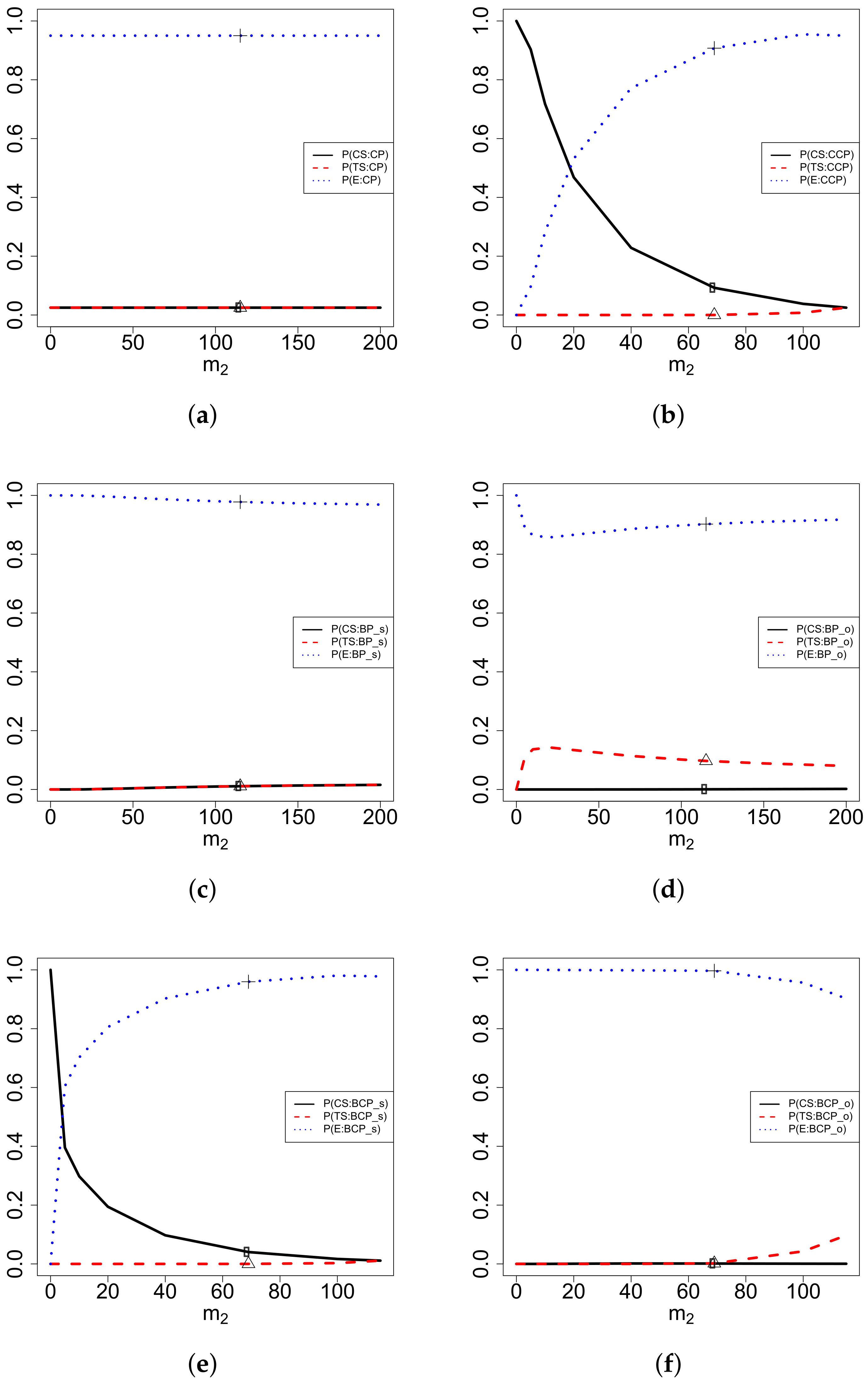
The upper left plot is for CP. We have

$$\underset{m_2\to 0^{+}}{lim}P\left(\mathrm{CS}:\mathrm{CP}\right)=\alpha ,\underset{m_2\to 0^{+}}{lim}P\left(\mathrm{TS}:\mathrm{CP}\right)=\alpha ,\underset{m_2\to 0^{+}}{lim}P\left(\mathrm{E}:\mathrm{CP}\right)=1-2\alpha .$$

Therefore, when $m_2$ is small (imprecision), the $P\left(\mathrm{E}:\mathrm{CP}\right)$ is large and it is hard to discriminate between CS and TS. Moreover, $P\left(\mathrm{CS}:\mathrm{CP}\right)$ is an increasing function of $m_2$, $P\left(\mathrm{TS}:\mathrm{CP}\right)$ is almost 0, and $P\left(\mathrm{E}:\mathrm{CP}\right)$ is a decreasing function of $m_2$. The three probabilities ($P\left(\mathrm{CS}:\mathrm{CP}\right)$, $P\left(\mathrm{TS}:\mathrm{CP}\right)$, and $P\left(\mathrm{E}:\mathrm{CP}\right)$) sum to 1.

(2)

The upper right plot is for CCP. We have

$$\underset{m_2\to 0^{+}}{lim}P\left(\mathrm{CS}:\mathrm{CCP}\right)=1,\underset{m_2\to 0^{+}}{lim}P\left(\mathrm{TS}:\mathrm{CCP}\right)=0,\underset{m_2\to 0^{+}}{lim}P\left(\mathrm{E}:\mathrm{CCP}\right)=0.$$

Therefore, when $m_2$ is small (imprecision), the $P\left(\mathrm{E}:\mathrm{CCP}\right)$ is small and it will predict CS. Moreover, $P\left(\mathrm{CS}:\mathrm{CCP}\right)$ is a first decreasing and then increasing function of $m_2$, $P\left(\mathrm{TS}:\mathrm{CCP}\right)$ is almost 0, and $P\left(\mathrm{E}:\mathrm{CCP}\right)$ is a first increasing and then decreasing function of $m_2$. The three probabilities ($P\left(\mathrm{CS}:\mathrm{CCP}\right)$, $P\left(\mathrm{TS}:\mathrm{CCP}\right)$, and $P\left(\mathrm{E}:\mathrm{CCP}\right)$) sum to 1.

(3)

The central left plot is for BP with a sceptical prior ($d_0={\mu }_s=0$). We have

$$\underset{m_2\to 0^{+}}{lim}P\left(\mathrm{CS}:\mathrm{BP}\_s\right)=0,\underset{m_2\to 0^{+}}{lim}P\left(\mathrm{TS}:\mathrm{BP}\_s\right)=0,\underset{m_2\to 0^{+}}{lim}P\left(E:\mathrm{BP}\_s\right)=1.$$

Therefore, when $m_2$ is small (imprecision), the $P\left(E:\mathrm{BP}\_s\right)$ is large and it is hard to discriminate between CS and TS. Moreover, $P\left(\mathrm{CS}:\mathrm{BP}\_s\right)$ is an increasing function of $m_2$, $P\left(\mathrm{TS}:\mathrm{BP}\_s\right)$ is almost 0, and $P\left(E:\mathrm{BP}\_s\right)$ is a decreasing function of $m_2$. The three probabilities ($P\left(\mathrm{CS}:\mathrm{BP}\_s\right)$, $P\left(\mathrm{TS}:\mathrm{BP}\_s\right)$, and $P\left(E:\mathrm{BP}\_s\right)$) sum to 1.

(4)

The central right plot is for BP with an optimistic prior ($d_0={\mu }_o=log0.6\approx -0.51$). We have

$$\underset{m_2\to 0^{+}}{lim}P\left(\mathrm{CS}:\mathrm{BP}\_o\right)=0,\underset{m_2\to 0^{+}}{lim}P\left(\mathrm{TS}:\mathrm{BP}\_o\right)=0,\underset{m_2\to 0^{+}}{lim}P\left(E:\mathrm{BP}\_o\right)=1.$$

Therefore, when $m_2$ is small (imprecision), the $P\left(E:\mathrm{BP}\_o\right)$ is large and it is hard to discriminate between CS and TS. Moreover, $P\left(\mathrm{CS}:\mathrm{BP}\_o\right)$ is an increasing function of $m_2$, $P\left(\mathrm{TS}:\mathrm{BP}\_o\right)$ is almost 0, and $P\left(E:\mathrm{BP}\_o\right)$ is a decreasing function of $m_2$. The three probabilities ($P\left(\mathrm{CS}:\mathrm{BP}\_o\right)$, $P\left(\mathrm{TS}:\mathrm{BP}\_o\right)$, and $P\left(E:\mathrm{BP}\_o\right)$) sum to 1.

(5)

The lower left plot is for BCP with a sceptical prior. We have

$$\underset{m_2\to 0^{+}}{lim}P\left(\mathrm{CS}:\mathrm{BCP}\_s\right)=1,\underset{m_2\to 0^{+}}{lim}P\left(\mathrm{TS}:\mathrm{BCP}\_s\right)=0,\underset{m_2\to 0^{+}}{lim}P\left(E:\mathrm{BCP}\_s\right)=0.$$

Therefore, when $m_2$ is small (imprecision), the $P\left(E:\mathrm{BCP}\_s\right)$ is small and it will predict CS. Moreover, $P\left(\mathrm{CS}:\mathrm{BCP}\_s\right)$ is a first decreasing and then increasing function of $m_2$, $P\left(\mathrm{TS}:\mathrm{BCP}\_s\right)$ is almost 0, and $P\left(E:\mathrm{BCP}\_s\right)$ is a first increasing and then decreasing function of $m_2$. The three probabilities ($P\left(\mathrm{CS}:\mathrm{BCP}\_s\right)$, $P\left(\mathrm{TS}:\mathrm{BCP}\_s\right)$, and $P\left(E:\mathrm{BCP}\_s\right)$) sum to 1.

(6)

The lower right plot is for BCP with an optimistic prior. We have

$$\underset{m_2\to 0^{+}}{lim}P\left(\mathrm{CS}:\mathrm{BCP}\_o\right)=0,\underset{m_2\to 0^{+}}{lim}P\left(\mathrm{TS}:\mathrm{BCP}\_o\right)=0,\underset{m_2\to 0^{+}}{lim}P\left(E:\mathrm{BCP}\_o\right)=1.$$

Therefore, when $m_2$ is small (imprecision), the $P\left(E:\mathrm{BCP}\_o\right)$ is large and it is hard to discriminate between CS and TS. Moreover, $P\left(\mathrm{CS}:\mathrm{BCP}\_o\right)$ is an increasing function of $m_2$, $P\left(\mathrm{TS}:\mathrm{BCP}\_o\right)$ is almost 0, and $P\left(E:\mathrm{BCP}\_o\right)$ is a decreasing function of $m_2$. The three probabilities ($P\left(\mathrm{CS}:\mathrm{BCP}\_o\right)$, $P\left(\mathrm{TS}:\mathrm{BCP}\_o\right)$, and $P\left(E:\mathrm{BCP}\_o\right)$) sum to 1.

(7)

The central two plots are for BP, with the left plot being a sceptical prior and the right plot being an optimistic prior. The two plots display similar patterns of increasing and decreasing characteristics. The sceptical prior favors control, and thus $P\left(\mathrm{CS}:\mathrm{BP}\_s\right)$ is larger than $P\left(\mathrm{CS}:\mathrm{BP}\_o\right)$. The optimistic prior favors treatment; however, the two probabilities ($P\left(\mathrm{TS}:\mathrm{BP}\_s\right)$ and $P\left(\mathrm{TS}:\mathrm{BP}\_o\right)$) for TS are almost 0, forcing $P\left(E:\mathrm{BP}\_o\right)tobe$ larger than $P\left(E:\mathrm{BP}\_s\right)$.

(8)

The lower two plots are for BCP, with the left plot being a sceptical prior and the right plot being an optimistic prior. The two plots display different patterns of increasing and decreasing characteristics. The sceptical prior favors control, and thus $P\left(\mathrm{CS}:\mathrm{BCP}\_s\right)$ is larger than $P\left(\mathrm{CS}:\mathrm{BCP}\_o\right)$. The optimistic prior favors treatment; however, the two probabilities ($P\left(\mathrm{TS}:\mathrm{BCP}\_s\right)$ and $P\left(\mathrm{TS}:\mathrm{BCP}\_o\right)$) for TS are almost 0, forcing $P\left(E:\mathrm{BCP}\_o\right)tobe$ larger than $P\left(E:\mathrm{BCP}\_s\right)$. The sceptical prior favors control and the interim data ($d_1^r$$=0.435$) also favors control, and thus, $P\left(\mathrm{CS}:\mathrm{BCP}\_s\right)$ is large. The optimistic prior favors treatment, but the interim data favors control, and thus, $P\left(E:\mathrm{BCP}\_o\right)$ is large.

(9)

The CP and BP do not utilize the interim data, and thus, the range of $m_2$ is $\left[0,200\right],$ with $m_2=s=115$ being marked in the plot (∘, ▵, and + for CS, TS, and E, respectively). The CCP and BCP utilize the interim data, and thus, the range of $m_2$ is $\left[0,s\right]=\left[0,115\right]$ with $m_2=m_2^r=69$ being marked in the plot (∘, ▵, and + for CS, TS, and E, respectively).

The probabilities of CS, TS, and E for CP, CCP, BP, and BCP as functions of $m_2$ when $\delta =1$, which favors control, are summarized in Web Table S1. This table reports the numerical values of the probabilities in Figure 3.

The probabilities of CS, TS, and E for CP, CCP, BP, and BCP as functions of $m_2$ when $\delta =-1$, which favors treatment, are plotted in Figure 4. From the figure, we observe the following facts.

(1)

Compared to Figure 3, since $\delta =1$ favors control and $\delta =-1$ favors treatment, the probabilities of CS in Figure 4 are smaller than those in Figure 3, while the probabilities of TS in Figure 4 are larger than those in Figure 3.

(2)

The central two plots are for BP, with the left plot being a sceptical prior and the right plot being an optimistic prior. The two plots display similar patterns of increasing and decreasing characteristics. The optimistic prior favors treatment, and thus, $P\left(\mathrm{TS}:\mathrm{BP}\_o\right)$ is larger than $P\left(\mathrm{TS}:\mathrm{BP}\_s\right)$. The sceptical prior favors control; however, the two probabilities ($P\left(\mathrm{CS}:\mathrm{BP}\_o\right)$ and $P\left(\mathrm{CS}:\mathrm{BP}\_s\right)$) for CS are almost 0, forcing $P\left(E:\mathrm{BP}\_s\right)tobe$ larger than $P\left(E:\mathrm{BP}\_o\right)$.

(3)

The lower two plots are for BCP, with the left plot being a sceptical prior and the right plot being an optimistic prior. The two plots display different patterns of increasing and decreasing characteristics. The sceptical prior favors control, and thus, $P\left(\mathrm{CS}:\mathrm{BCP}\_s\right)$ is larger than $P\left(\mathrm{CS}:\mathrm{BCP}\_o\right)$. The optimistic prior favors treatment, and thus, $P\left(\mathrm{TS}:\mathrm{BCP}\_o\right)$ is larger than $P\left(\mathrm{TS}:\mathrm{BCP}\_s\right)$. The sceptical prior favors control and the interim data ($d_1^r$$=0.435$) also favors control, and thus, $P\left(\mathrm{CS}:\mathrm{BCP}\_s\right)$ is large. The optimistic prior favors treatment but the interim data favors control, and thus, $P\left(E:\mathrm{BCP}\_o\right)$ is large.

The probabilities of CS, TS, and E for CP, CCP, BP, and BCP as functions of $m_2$ when $\delta =-1$ which favors treatment, are summarized in Web Table S2. This table reports the numerical values of the probabilities in Figure 4.

The probabilities of CS, TS, and E for CP, CCP, BP, and BCP as functions of $m_2$ when $\delta =0$, which favors equivocal, are plotted in Figure 5. From the figure, we observe the following facts.

(1)

Compared to Figure 3 and Figure 4, since $\delta =0$ favors equivocal, the probabilities of equivocal in Figure 5 are larger than those in Figure 3 and Figure 4 for CP, BP_s, BP_o, and BCP_o. It is interesting to note that for $P\left(\mathrm{E}:\mathrm{CCP}\right)$ in Figure 4, the interim data favors control and $\delta =-1$ favors treatment, and thus, $P\left(\mathrm{E}:\mathrm{CCP}\right)$ in Figure 4 is large. Similarly, for $P\left(E:\mathrm{BCP}\_s\right)$ in Figure 4, the interim data favors control, the sceptical prior favors control, and $\delta =-1$ favors treatment, and thus, $P\left(E:\mathrm{BCP}\_s\right)$ in Figure 4 is large. Nevertheless, the $P\left(\mathrm{E}:\mathrm{CCP}\right)$ and $P\left(E:\mathrm{BCP}\_s\right)$ in Figure 5 are large, since $\delta =0$ favors equivocal in this figure.

(2)

The central two plots are for BP, with the left plot being a sceptical prior and the right plot being an optimistic prior. The two plots display different patterns of increasing and decreasing characteristics. The sceptical prior favors control, and thus, $P\left(CS:\mathrm{BP}\_s\right)$ is larger than $P\left(CS:\mathrm{BP}\_o\right)$. The optimistic prior favors treatment, and thus, $P\left(TS:\mathrm{BP}\_o\right)$ is larger than $P\left(TS:\mathrm{BP}\_s\right)$.

(3)

The lower two plots are for BCP, with the left plot being a sceptical prior and the right plot being an optimistic prior. The two plots display different patterns of increasing and decreasing characteristics. The sceptical prior favors control, and thus, $P\left(CS:\mathrm{BCP}\_s\right)$ is larger than $P\left(CS:\mathrm{BCP}\_o\right)$. The optimistic prior favors treatment, and thus, $P\left(TS:\mathrm{BCP}\_o\right)$ is larger than $P\left(TS:\mathrm{BCP}\_s\right)$. The sceptical prior favors control and the interim data ($d_1^r$$=0.435$) also favors control, and thus, $P\left(CS:\mathrm{BCP}\_s\right)$ is large. The optimistic prior favors treatment, but the interim data favors control, and thus, $P\left(E:\mathrm{BCP}\_o\right)$ is large.

Comparing Figure 3, Figure 4 and Figure 5, we see that

$$\begin{array}{cc}\hfill \underset{m_2\to 0^{+}}{lim}P\left(\mathrm{CS}:\mathrm{CP}\right)& =\alpha ,\underset{m_2\to 0^{+}}{lim}P\left(\mathrm{TS}:\mathrm{CP}\right)=\alpha ,\underset{m_2\to 0^{+}}{lim}P\left(\mathrm{E}:\mathrm{CP}\right)=1-2\alpha ,\hfill \\ \hfill \underset{m_2\to 0^{+}}{lim}P\left(\mathrm{CS}:\mathrm{CCP}\right)& =1,\underset{m_2\to 0^{+}}{lim}P\left(\mathrm{TS}:\mathrm{CCP}\right)=0,\underset{m_2\to 0^{+}}{lim}P\left(\mathrm{E}:\mathrm{CCP}\right)=0,\hfill \\ \hfill \underset{m_2\to 0^{+}}{lim}P\left(CS:\mathrm{BP}\_s\right)& =0,\underset{m_2\to 0^{+}}{lim}P\left(TS:\mathrm{BP}\_s\right)=0,\underset{m_2\to 0^{+}}{lim}P\left(ES:\mathrm{BP}\_s\right)=1,\hfill \\ \hfill \underset{m_2\to 0^{+}}{lim}P\left(CS:\mathrm{BP}\_o\right)& =0,\underset{m_2\to 0^{+}}{lim}P\left(TS:\mathrm{BP}\_o\right)=0,\underset{m_2\to 0^{+}}{lim}P\left(E:\mathrm{BP}\_o\right)=1,\hfill \\ \hfill \underset{m_2\to 0^{+}}{lim}P\left(CS:\mathrm{BCP}\_s\right)& =1,\underset{m_2\to 0^{+}}{lim}P\left(TS:\mathrm{BCP}\_s\right)=0,\underset{m_2\to 0^{+}}{lim}P\left(E:\mathrm{BCP}\_s\right)=0,\hfill \\ \hfill \underset{m_2\to 0^{+}}{lim}P\left(CS:\mathrm{BCP}\_o\right)& =0,\underset{m_2\to 0^{+}}{lim}P\left(TS:\mathrm{BCP}\_o\right)=0,\underset{m_2\to 0^{+}}{lim}P\left(E:\mathrm{BCP}\_o\right)=1,\hfill \end{array}$$

regardless of the $\delta$ values, as the comparison variables and the threshold variables of all the limits do not depend on $\delta$. Therefore, the CP, BP_s, BP_o, and BCP_o have imprecision issues.

The probabilities of CS, TS, and E for CP, CCP, BP, and BCP as functions of $m_2$ when $\delta =0$, which favors equivocal, are summarized in Web Table S3. This table reports the numerical values of the probabilities in Figure 5.

The probabilities of CS, TS, and E for the eight predictive powers as functions of $m_2$ under the sceptical prior are plotted in Web Figure S2 and summarized in Web Table S4.

The probabilities of CS, TS, and E for the eight predictive powers as functions of $m_2$ under the optimistic prior are plotted in Web Figure S3 and summarized in Web Table S5.

4. A Real Data Example

In this section, we perform some numerical experiments on a real data example. First, we will compute the probabilities of CS, TS, and E for CP, CCP, BP_s, BP_o, BCP_s, and BCP_o when $\delta =1$ (favors control), $-1$ (favors treatment), and 0 (favors equivocal), respectively. Second, we will compute the probabilities of CS, TS, and E for the eight predictive powers under either a sceptical or optimistic prior.

Long-term tamoxifen therapy is used to prevent the recurrence of breast cancer (see [5]; Example 6.7 in [15,16]). The aim of this study is to estimate disease-free survival benefit from tamoxifen over placebo, in patients who already have had 5 years of taking tamoxifen without a recurrence. It implies that patients were randomized to either continuation with placebo vs. continuation with tamoxifen therapy after having survived recurrence-free under tamoxifen for 5 years. So as to detect a $40\%$ reduction in annual risk associated with tamoxifen (hazard ratio $=0.6$), with $85\%$ power and a one-sided tail area of $5\%$, 115 events were required. With summary using the approximate hazard ratio analysis, the proportional hazards regression model is the statistical model. If there are $O_T$ events on treatment, and $O_C$ events on control, then $d_1=2(O_T-O_C)/m_1$ is an approximate estimate of the log(hazard ratio) $\delta$, with mean $\delta$ and variance $4/m_1$, as shown in [17]. There are two prior distributions that are used. An optimistic prior was centered on a $40\%$ hazard reduction and a $5\%$ chance of a negative effect (i.e., $HR>1$), equivalent on the $log\left(HR\right)$ scale to a normal prior with mean ${\mu }_o=log\left(0.6\right)=-0.51$ and standard deviation $0.31$ ($\sigma =\sqrt{2}$, $m_0=41.4$). It is useful to note that in [15], the variance is ${\sigma }^2=4$, while in this article, the variance is $2{\sigma }^2=4$, and thus, $\sigma =\sqrt{2}$ in this article. In addition, a sceptical prior was adopted with the same standard deviation as the optimistic prior, but centered on ${\mu }_s=0$. The estimated $log\left(HR\right)$ after the first interim analysis in 1993 is $d_1=0.435$; at that time, $m_1=46$ events have been observed, and a further $m_2=115-46=69$ events are to be observed. The chosen significance level $\alpha$ is $0.025$. Therefore, we have

$$\alpha =0.025,\sigma =\sqrt{2},{\mu }_s=0,{\mu }_o=log\left(0.6\right)=-0.51,s=115,d_1=0.435,$$

$$m_0=41.4,m_1=46,m_2\left\{\begin{array}{cc}=s=115,\hfill & \mathrm{for}i=1,5,\hfill \\ =s-m_1=69,\hfill & \mathrm{for}i=2,3,4,6,7,8.\hfill \end{array}\right.$$

The probabilities of CS, TS, and E for CP, CCP, BP_s, BP_o, BCP_s, and BCP_o when $\delta =1$ (favors control), $-1$ (favors treatment), and 0 (favors equivocal) are summarized in

Table 2. The probabilities of CS, TS, and E for CP, CCP, BP_s, BP_o, BCP_s, and BCP_o when $\delta =1$ (favors control), $-1$ (favors treatment), and 0 (favors equivocal).

		CS	TS	E
$\delta =1$	CP	$0.986$	$0.000$	$0.014$
	CCP	$0.998$	$0.000$	$0.002$
	$BP\_s$	$0.953$	$0.000$	$0.047$
	$BP\_o$	$0.655$	$0.000$	$0.345$
	$BCP\_s$	$0.992$	$0.000$	$0.008$
	$BCP\_o$	$0.871$	$0.000$	$0.129$
$\delta =-1$	CP	$0.000$	$0.986$	$0.014$
	CCP	$0.000$	$0.662$	$0.338$
	$BP\_s$	$0.000$	$0.953$	$0.047$
	$BP\_o$	$0.000$	$0.998$	$0.002$
	$BCP\_s$	$0.000$	$0.499$	$0.501$
	$BCP\_o$	$0.000$	$0.898$	$0.102$
$\delta =0$	CP	$0.025$	$0.025$	$0.950$
	CCP	$0.092$	$0.000$	$0.907$
	$BP\_s$	$0.007$	$0.007$	$0.987$
	$BP\_o$	$0.000$	$0.114$	$0.886$
	$BCP\_s$	$0.040$	$0.000$	$0.960$
	$BCP\_o$	$0.001$	$0.002$	$0.997$

. From the table, we observe the following facts.

(1)

In each row, the sum of the three probabilities should be equal to 1. However, in some circumstances, the sum is equal to $0.999$, due to the rounding error.

(2)

When $\delta =1$, which favors control, the probabilities of CS are large for CP, CCP, BP_s, BP_o, BCP_s, and BCP_o; when $\delta =-1$, which favors treatment, the probabilities of TS are large for CP, CCP, BP_s, BP_o, BCP_s, and BCP_o; and when $\delta =0$, which favors equivocal, the probabilities of E are large for CP, CCP, BP_s, BP_o, BCP_s, and BCP_o. In conclusion, for a given true condition (CS, TS, or E), the probabilities of that condition (CS, TS, or E) are large for CP, CCP, BP_s, BP_o, BCP_s, and BCP_o.

(3)

CP, BP_s, BP_o, and BCP_o have imprecision issues, while CCP and BCP_s do not have imprecision issues (see Figure 3, Figure 4 and Figure 5). However, for all the powers, the probabilities of E are large only when $\delta =0$, which favors equivocal. That is to say, when $\delta =1$ (favors control) and $\delta =-1$ (favors treatment), the probabilities of E are not large for all the powers (an exception is the probability of E, which is equal to $0.501$ for BCP_s when $\delta =-1$). Therefore, whether the probabilities of E are large are affected by the $\delta$ values, but are not affected by whether the power has an imprecision issue.

The probabilities of CS, TS, and E for the eight predictive powers under the sceptical or optimistic prior are summarized in

Table 3. The probabilities of CS, TS, and E for the eight predictive powers under the sceptical or optimistic prior.

	CS		TS		E
PPs	Sceptical	Optimistic	Sceptical	Optimistic	Sceptical	Optimistic
$I_1$	$0.156$	$0.008$	$0.156$	$0.656$	$0.687$	$0.336$
$I_2$	$0.225$	$0.066$	$0.015$	$0.077$	$0.760$	$0.857$
$I_3$	$0.208$	$0.017$	$0.011$	$0.161$	$0.781$	$0.821$
$I_4$	$0.389$	$0.151$	$0.000$	$0.003$	$0.610$	$0.846$
$I_5$	$0.120$	$0.001$	$0.120$	$0.771$	$0.761$	$0.228$
$I_6$	$0.126$	$0.002$	$0.005$	$0.195$	$0.869$	$0.803$
$I_7$	$0.142$	$0.001$	$0.005$	$0.321$	$0.852$	$0.678$
$I_8$	$0.276$	$0.011$	$0.000$	$0.017$	$0.724$	$0.972$

. From the table, we observe the following facts.

(1)

In each row, the sum of the three probabilities corresponding to the sceptical prior (or the optimistic prior) should be equal to 1. However, in some cases, the sum is equal to $0.999$, due to the rounding error.

(2)

For the eight predictive powers, $I_1$_s, $I_2$_s, $I_5$_s, $I_6$_s, $I_1$_o, $I_2$_o, $I_5$_o, $I_6$_o, $I_7$_o, and $I_8$_o have imprecision issues; however, $I_3$_s, $I_4$_s, $I_7$_s, $I_8$_s, $I_3$_o, and $I_4$_o do not have imprecision issues (see Web Figures S2 and S3). Moreover, the probabilities of E are large for all the eight predictive powers under the sceptical or optimistic prior except $I_1$_o and $I_5$_o. It is common that having an imprecision issue combines with $P\left(\mathrm{E}\right)$ large; for instance, $I_1$_s, $I_2$_s, $I_5$_s, $I_6$_s, $I_2$_o, $I_6$_o, $I_7$_o, and $I_8$_o. However, not having an imprecision issue may combine with $P\left(\mathrm{E}\right)$ large; for example, $I_3$_s, $I_4$_s, $I_7$_s, $I_8$_s, $I_3$_o, and $I_4$_o. Moreover, having an imprecision issue may combine with $P\left(\mathrm{E}\right)$ small; for instance, $I_1$_o and $I_5$_o. Therefore, whether the probabilities of E are large is not affected by whether the predictive power has an imprecision issue.

(3)

Note that the numerical values of this table are the same as those of Table 3 in [5]. However, in this table, we have discussed that the relationship between the imprecision issue of the predictive power and the probability of E large, and the relationship is described in item (2).

(4)

At the interim, the trial is stopped for futility, because the probabilities of TS are small for all the six predictive powers at the interim ($I_2$, $I_3$, $I_4$, $I_6$, $I_7$, and $I_8$). However, it is not because the probabilities of CS are large, but because the probabilities of E are large. In a word, at the interim, the trial neither favors treatment nor control, but favors equivocal.

5. Conclusions and Discussions

Some conclusions and discussions are provided below.

• We have derived the probabilities of CS, TS, and E of the four powers and the eight predictive powers, and have evaluated the limits of the probabilities at point 0. Moreover, we have conducted extensive numerical experiments to exemplify the imprecision issues of the four powers and the eight predictive powers. In the numerical experiments, first, we have computed the probabilities of CS, TS, and E for the four powers as functions of $m_2$ when the true treatment effect favors control, treatment, and equivocal, respectively. Second, we have computed the probabilities of CS, TS, and E for the eight predictive powers as functions of $m_2$ under the sceptical prior and the optimistic prior, respectively. Finally, we have carried out a real data example to show the prominence of the methods.
• For the four powers and the eight predictive powers with the parameters specified in (19), some have imprecision issues, but the others do not have these issues. More precisely, the CP, BP_s, BP_o, BCP_o, $I_1$_s, $I_2$_s, $I_5$_s, $I_6$_s, $I_1$_o, $I_2$_o, $I_5$_o, $I_6$_o, $I_7$_o, and $I_8$_o have imprecision issues. However, the CCP, BCP_s, $I_3$_s, $I_4$_s, $I_7$_s, $I_8$_s, $I_3$_o, and $I_4$_o do not have imprecision issues.
• In fact, each of the four powers and the eight predictive powers has an opportunity to encounter the imprecision issue as long as the parameter values are chosen appropriately. Firstly, from (6), we see that the CP, $I_1$, and $I_2$ will certainly have imprecision issues. Moreover, from (10), we see that if

  $$-Z_{\alpha }\sigma \sqrt{2/s}<d_1<Z_{\alpha }\sigma \sqrt{2/s},$$

  then the CCP, $I_3$, and $I_4$ will have imprecision issues. Furthermore, from (14), we see that if

  $$-Z_{\alpha }\sigma \sqrt{2/m_0}<d_0<Z_{\alpha }\sigma \sqrt{2/m_0},$$

  then the BP, $I_5$, and $I_6$ will have imprecision issues. Finally, from (18), we see that if

  $$-Z_{\alpha }\sigma \sqrt{2\left(m_0+s\right)}<m_0{d}_0+s{d}_1<Z_{\alpha }\sigma \sqrt{2\left(m_0+s\right)},$$

  then the BCP, $I_7$, and $I_8$ will have imprecision issues.
• For simplicity, let

  $$P\left(\mathrm{CS}\right)=P\left(\mathrm{CS}:i\right),P\left(\mathrm{TS}\right)=P\left(\mathrm{TS}:i\right),\mathrm{and}P\left(\mathrm{E}\right)=P\left(\mathrm{E}:i\right),$$

  where $i=$ CP, CCP, BP_s, BP_o, BCP_s, BCP_o, $I_j$_s, and $I_j$_o for $j=1,\dots ,8$. We say that

  $$\begin{array}{cc}\hfill P\left(\mathrm{E}\right)\mathrm{is}\mathrm{large}& \iff P\left(\mathrm{E}\right)=max\left\{P\left(\mathrm{CS}\right),P\left(\mathrm{TS}\right),P\left(\mathrm{E}\right)\right\},\hfill \\ \hfill P\left(\mathrm{E}\right)\mathrm{is}\mathrm{small}& \iff P\left(\mathrm{E}\right)\ne max\left\{P\left(\mathrm{CS}\right),P\left(\mathrm{TS}\right),P\left(\mathrm{E}\right)\right\},\hfill \end{array}$$

  where the comparison is for the same power or predictive power. Similarly, we say that

  $$\begin{array}{cc}\hfill P\left(\mathrm{CS}\right)\mathrm{is}\mathrm{large}& \iff P\left(\mathrm{CS}\right)=max\left\{P\left(\mathrm{CS}\right),P\left(\mathrm{TS}\right),P\left(\mathrm{E}\right)\right\},\hfill \\ \hfill P\left(\mathrm{CS}\right)\mathrm{is}\mathrm{small}& \iff P\left(\mathrm{CS}\right)\ne max\left\{P\left(\mathrm{CS}\right),P\left(\mathrm{TS}\right),P\left(\mathrm{E}\right)\right\},\hfill \\ \hfill P\left(\mathrm{TS}\right)\mathrm{is}\mathrm{large}& \iff P\left(\mathrm{TS}\right)=max\left\{P\left(\mathrm{CS}\right),P\left(\mathrm{TS}\right),P\left(\mathrm{E}\right)\right\},\hfill \\ \hfill P\left(\mathrm{TS}\right)\mathrm{is}\mathrm{small}& \iff P\left(\mathrm{TS}\right)\ne max\left\{P\left(\mathrm{CS}\right),P\left(\mathrm{TS}\right),P\left(\mathrm{E}\right)\right\}.\hfill \end{array}$$
• For the powers with the parameters specified in (19), CP, BP_s, BP_o, and BCP_o have imprecision issues, while CCP and BCP_s do not have imprecision issues. For all the powers (CP, CCP, BP_s, BP_o, BCP_s, and BCP_o), when the true condition favors control ($\delta =1$ in Figure 3), the $P\left(\mathrm{CS}\right)$ is large on the marker (∘ for CS); when the true condition favors treatment ($\delta =-1$ in Figure 4), the $P\left(\mathrm{TS}\right)$ is large on the marker (▵ for TS); and when the true condition favors equivocal ($\delta =0$ in Figure 5), the $P\left(\mathrm{E}\right)$ is large on the marker (+ for E). We discover that whether the power has an imprecision issue is not related to whether $P\left(\mathrm{E}\right)$ is large or not on the marker.
• It is important to point out that the statement that the predictive power has an imprecision issue is different from the statement that $P\left(\mathrm{E}\right)$ is large on the marker (+ for E). An imprecision issue means that when $m_2$ is small (imprecision), $P\left(\mathrm{E}\right)$ is large. However, $P\left(\mathrm{E}\right)$ is large on the marker, which does not require a small or large $m_2$. It is common that having an imprecision issue combines with $P\left(\mathrm{E}\right)$ large on the marker; for instance, $I_1$_s, $I_2$_s, $I_5$_s, and $I_6$_s in Web Figure S2, and $I_2$_o, $I_6$_o, $I_7$_o, and $I_8$_o in Web Figure S3. However, not having an imprecision issue may combine with $P\left(\mathrm{E}\right)$ large on the marker; for example, $I_3$_s, $I_4$_s, $I_7$_s, and $I_8$_s in Web Figure S2, and $I_3$_o and $I_4$_o in Web Figure S3. Moreover, having an imprecision issue may combine with $P\left(\mathrm{E}\right)$ small on the marker, for instance, $I_1$_o and $I_5$_o in Web Figure S3.
• It is worth noting that the CP in this article means Classical Power, which should not be confused with Conditional Power in the literature (see [18,19,20,21,22,23]).

References

- Choi, S.C.; Smith, P.J.; Becker, D.P. Early decision in clinical trials when the treatment differences are small. Control. Clin. Trials 1985, 6, 280–288. [Google Scholar] [CrossRef]
- Spiegelhalter, D.J.; Freedman, L.S.; Blackburn, P.R. Monitoring clinical trials: Conditional or predictive power? Control. Clin. Trials 1986, 7, 8–17. [Google Scholar] [CrossRef]
- Schmidli, H.; Bretz, F.; Racine-Poon, A. Bayesian predictive power for interim adaptation in seamless phase II/III trials where the endpoint is survival up to some specified timepoint. Stat. Med. 2007, 26, 4925–4938. [Google Scholar] [CrossRef] [PubMed]
- Zhang, Y.Y.; Ting, N. Bayesian sample size determination for a phase III clinical trial with diluted treatment effect. J. Biopharm. Stat. 2018, 28, 1119–1142. [Google Scholar] [CrossRef]
- Zhang, Y.Y.; Rong, T.Z.; Li, M.M. Eight predictive powers with historical and interim data for futility and efficacy analysis. Stat. Theory Relat. Fields 2022. [Google Scholar] [CrossRef]
- O’Hagan, A.; Stevens, J.W.; Campbell, M.J. Assurance in clinical trial design. Pharm. Stat. 2005, 4, 187–201. [Google Scholar] [CrossRef]
- Wang, S.J.; Hung, H.M.J.; O’Neill, R.T. Adapting the sample size planning of a phase III trial based on phase II data. Pharm. Stat. 2006, 5, 85–97. [Google Scholar] [CrossRef]
- Kirby, S.; Burke, J.; Chuang-Stein, C.; Sin, C. Discounting phase 2 results when planning phase 3 clinical trials. Pharm. Stat. 2012, 11, 373–385. [Google Scholar] [CrossRef]
- Trzaskoma, B.; Sashegyi, A. Predictive probability of success and the assessment of futility in large outcomes trials. J. Biopharm. Stat. 2007, 17, 45–63. [Google Scholar] [CrossRef]
- Jiang, K. Optimal sample sizes and go/no-go decisions for phase II/III development programs based on probability of success. Stat. Biopharm. Res. 2011, 3, 463–475. [Google Scholar] [CrossRef]
- Ibrahim, J.G.; Chen, M.H.; Lakshminarayanan, M.; Liu, G.F.; Heyse, J.F. Bayesian probability of success for clinical trials using historical data. Stat. Med. 2015, 34, 249–264. [Google Scholar] [CrossRef]
- Chuang-Stein, C. Sample size and the probability of a successful trial. Pharm. Stat. 2006, 5, 305–309. [Google Scholar] [CrossRef]
- Zhang, Y.Y.; Ting, N. Sample size considerations for a phase III clinical trial with diluted treatment effect. Stat. Biopharm. Res. 2020, 12, 311–321. [Google Scholar] [CrossRef]
- Zhang, Y.Y.; Rong, T.Z.; Li, M.M. The contemplated average success probability for normally distributed models with an application to optimal sample sizes selection. Stat. Med. 2020, 39, 3173–3183. [Google Scholar] [CrossRef]
- Spiegelhalter, D.J.; Abrams, K.R.; Myles, J.P. Bayesian Approaches to Clinical Trials and Health-Care Evaluation; Wiley: Chichester, UK, 2004. [Google Scholar]
- Dignam, J.J.; Bryant, J.; Wieand, H.S.; Fisher, B.; Wolmark, N. Early stopping of a clinical trial when there is evidence of no treatment benefit: Protocol B-14 of the National Surgical Adjuvant Breast and Bowel Project. Control. Clin. Trials 1998, 19, 575–588. [Google Scholar] [CrossRef]
- Tsiatis, A.A. The asymptotic joint distribution of the efficient scores test for the proportional hazards model calculated over time. Biometrika 1981, 68, 311–315. [Google Scholar] [CrossRef]
- Lachin, J.M. A review of methods for futility stopping based on conditional power. Stat. Med. 2005, 24, 2747–2764. [Google Scholar] [CrossRef]
- Lachin, J.M. Operating characteristics of sample size re-estimation with futility stopping based on conditional power. Stat. Med. 2006, 25, 3348–3365. [Google Scholar] [CrossRef]
- Lan, K.K.G.; Hu, P.; Proschan, M.A. A conditional power approach to the evaluation of predictive power. Stat. Biopharm. Res. 2009, 1, 131–136. [Google Scholar] [CrossRef]
- Zhang, Y.; Clarke, W.R. A flexible futility monitoring method with time-varying conditional power boundary. Clin. Trials 2010, 7, 209–218. [Google Scholar] [CrossRef]
- Ciolino, J.D.; Martin, R.H.; Zhao, W.L.; Jauch, E.C.; Hill, M.D.; Palesch, Y.Y. Continuous covariate imbalance and conditional power for clinical trial interim analyses. Contemp. Clin. Trials 2014, 38, 9–18. [Google Scholar] [CrossRef]
- Deng, Q.Q.; Zhang, Y.Y.; Roy, D.; Chen, M.H. Superiority of combining two independent trials in interim futility analysis. Stat. Methods Med. Res. 2020, 29, 522–540. [Google Scholar] [CrossRef]