Optimizing Echo State Networks for Enhancing Large Prediction Horizons of Chaotic Time Series

Abstract

Reservoir computing has shown promising results in predicting chaotic time series. However, the main challenges of time-series predictions are associated with reducing computational costs and increasing the prediction horizon. In this sense, we propose the optimization of Echo State Networks (ESN), where the main goal is to increase the prediction horizon using a lower count number of neurons compared with state-of-the-art models. In addition, we show that the application of the decimation technique allows us to emulate an increase in the prediction of up to 10,000 steps ahead. The optimization is performed by applying particle swarm optimization and considering two chaotic systems as case studies, namely the chaotic Hindmarsh–Rose neuron with slow dynamic behavior and the well-known Lorenz system. The results show that although similar works used from 200 to 5000 neurons in the reservoir of the ESN to predict from 120 to 700 steps ahead, our optimized ESN including decimation used 100 neurons in the reservoir, with a capability of predicting up to 10,000 steps ahead. The main conclusion is that we ensured larger prediction horizons compared to recent works, achieving an improvement of more than one order of magnitude, and the computational costs were greatly reduced.

1. Introduction

Nowadays, the prediction of chaotic time series remains an open challenge. Some well-known applications are, for example, weather predictions [1,2,3], health-related pathologies [4], and financial procedures [5], among others. In particular, these cases exhibit chaotic behavior that is often modeled by sets of strongly coupled nonlinear differential equations [6] so that their solutions depend on the dynamic characteristics, which have high sensitivity to the initial conditions, i.e., the solutions of two identical chaotic systems with slight differences in the initial conditions will be significantly different after a brief evolution time [7]. Fortunately, some works provide guidelines to solve these types of chaotic systems by applying appropriate numerical methods [8].

Due to the difficulties in modeling chaotic systems, promising techniques such as machine learning (ML) as universal approximations of nonlinear functions are employed to learn the behavior of chaotic systems from experimental data, making predictions of the time series without specific knowledge of the model [9]. Some ML techniques that are applied to chaotic time series predictions are support vector machine (SVM) [10], artificial neural networks (ANN), recurrent neural networks with long short-term memory (RNN-LSTM) [6], feedforward neural networks [11,12], and reservoir computing (RC) [13,14,15,16], among others. The RC technique is one of the most commonly used for predicting chaotic time series, as shown in [6,17,18], where the authors compared RC with ANN and RNN-LSTM, showing that RC predicted a more significant number of steps ahead. Some improvements to RC, such as including a knowledge-based model (hybrid model) [19], increased the prediction time almost twofold. In this sense, the main challenges are related to how to increase the prediction horizon and reduce computing costs. To cope with these issues, different alternatives were explored in [20], where the authors proposed a robust Echo State Network (ESN) by replacing the Gaussian likelihood function in the Bayesian regression with a Laplace likelihood function. In [21], the authors carried out a Bayesian optimization of the reservoir hyperparameters (leaking rate, spectral radius, etc.) since selecting them is difficult due to all the possible combinations. In [22], the authors also used Bayesian optimization to find a good set of hyperparameters for the ESN and proposed a cross-validation method to validate their results. In [23], one can see the application of a backtracking search optimization algorithm (BSA) and its variants to determine the most appropriate output weights of an ESN given that the optimization problem was complex. In [24], the authors optimized the ESN input matrix, which was randomly defined in the original proposal [25], using the selective opposition gray wolf algorithm. Recently, in [26], an ESN with improved topology was proposed for accurate and efficient time-series predictions using a smooth reservoir activation function. The prediction times increased in all of these cases but the study systems were still lacking in some aspects. For example, they did not include slow-behavior chaotic systems as artificial neurons, where the change in amplitude between the current point and the previous one was small, tending to be monotone or periodic.

In this work, we show the time-series predictions of two chaotic systems, namely the Lorenz system [27] and the Hindmarsh–Rose neuron (HRN), which has slow dynamic behavior [28]. We show the use of ESNs as an ML technique with the goal of improving the prediction horizon. The horizon is highly improved by decimating the time series without affecting its dynamical characteristics, such as the Lyapunov spectrum and Kaplan–Yorke dimension. The prediction horizon is also increased by optimizing the reservoir input matrix of the ESN ${\mathbf{W}}_{\mathbf{in}}$, applying the particle swarm optimization (PSO) algorithm. It is highlighted that in all the experiments, our work considers a small reservoir size compared to similar works, making our proposal more efficient in terms of computational costs. The paper concludes by showing a comparison of our results and related studies, observing a similar or even a much better prediction horizon with very few neurons. The remainder of the document is structured as follows. Section 2, describes the topology of the ESN and PSO algorithms. Section 3 describes the datasets used for the times-series prediction. Section 4 presents the technique for the chaotic time-series prediction using ESN without optimization. Section 5 shows the prediction results of the optimized ESN with different decimation cases. Finally, the conclusions are summarized in Section 6.

2. ESN and PSO Algorithms

2.1. Echo State Network

In general, the basic structure of an ESN consists of an input layer, an internal reservoir network containing N nodes in the hidden layer, and an output layer [24]. One recommendation is that N is in the range $(\frac{T}{10}\le N\le \frac{T}{2})$, with T being the number of sample data [29]. For optimization purposes, the optimal value of N depends on the periodicity of the training data and learning task complexity. A reservoir size that is too small may cause model inaccuracy, whereas a reservoir size that is too large may lead to slow training and data overfitting [30]. The ESN topology is shown in Figure 1, where ${\mathbf{W}}_{\mathbf{in}}\in {\mathbb{R}}^{N_x\times (1+N_u)}$ is the input weight matrix; $\mathbf{W}\in {\mathbb{R}}^{N_x\times N_x}$ is the recurrent weight matrix in the reservoir; $u\left(t\right)\in {\mathbb{R}}^{N_u}$ is the input signal; $y\left(t\right)\in {\mathbb{R}}^{N_y}$ is the network output; $\mathbf{x}\left(t\right)\in {\mathbb{R}}^{N_x}$ is the state vector of the reservoir neuron activations; and $t=1,\cdots ,T$ denotes the discrete time.

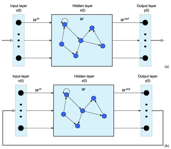
Figure 1. Generic topology of an Echo State Network. (a) Training stage, and (b) Prediction stage.

The leaky integrator ESN is the most frequently used variant. The state vector update equation is described by (1), where parameter $a\in (0,1]$ is the leaking rate, and this parameter controls the update speed of the reservoir state vector $\mathbf{x}\left(\mathbf{t}\right)$. In [31], some considerations are given to select this parameter, where the authors suggest that the gain $\left(\gamma \right)$ be 1.

$$\mathbf{x}(t+1)=(1-a\gamma )\mathbf{x}\left(t\right)+\gamma f(\mathbf{Wx}\left(t\right)+{\mathbf{W}}_{\mathbf{in}}[b_{in};u\left(t\right)])$$

(1)

The new state vector update is given in (2), where $b_{in}=1$ is the input bias value, f is an activation function such as $tanh(·)$, and ${\mathbf{W}}_{\mathbf{in}}$ and $\mathbf{W}$ are the weight matrices generated randomly from a uniform distribution in $[-1,1]$ when the reservoir was initially established. The matrix $\mathbf{W}$ must be re-scaled to a sparse matrix with a spectral radius $\left({\rho }_r\right)$ less than or equal to 1 [21], according to (3) to guarantee the echo state property [32].

$$\mathbf{x}(t+1)=(1-a)\mathbf{x}\left(t\right)+f(\mathbf{Wx}\left(t\right)+{\mathbf{W}}_{\mathbf{in}}[b_{in};u\left(t\right)])$$

(2)

$${\mathbf{W}}_{\mathbf{r}}=\frac{{\rho }_r}{{\rho }_r\left(\mathbf{W}\right)}\mathbf{W}$$

(3)

In the training stage shown in Figure 1a, the main goal is to minimize the error between $y\left(t\right)$ and the target output $y^{target}\left(t\right)$. The output weight matrix ${\mathbf{W}}_{\mathbf{out}}$ is the parameter “trainable” and it is available just after the training stage. Equation (4) describes this matrix, where $\lambda$ is the regularization coefficient of the reservoir, which is used to prevent overfitting. $\mathbf{X}\in {\mathbb{R}}^{(1+N_u+N_x)\times T}$ is the matrix collecting all column-vectors $[1;u(t);\mathbf{x}(\mathbf{t}\left)\right]$ by concatenating horizontally during the training period $t=1,\cdots ,T$.

$${\mathbf{W}}_{\mathbf{out}}=y^{target}{\mathbf{X}}^{\mathbf{T}}{(\mathbf{X}{\mathbf{X}}^T+\lambda \mathbf{I})}^{-1}$$

(4)

In the prediction stage shown in Figure 1b, the current output is the feedback and is used as the input $u\left(t\right)$ to predict the next value using (5), where $b_{out}=1$ is the output bias value; the rest of the elements are part of a vertical vector (or matrix) concatenation.

$$y(t+1)={\mathbf{W}}_{\mathbf{out}}[b_{out};u\left(t\right);\mathbf{x}\left(\mathbf{t}\right)]$$

(5)

2.2. Particle Swarm Optimization (PSO) Algorithm

In the basic PSO algorithm, the particle swarm consists of n particles, and the position of each particle stands for the potential solution in D-dimensional space [33]. The PSO algorithm is simple in concept, easy to implement, and computationally efficient. The original procedure for implementing the PSO is as follows:

1.

Initialize a population of particles with random positions and velocities on D-dimensions in the problem space.

2.

For each particle, evaluate the desired optimization fitness function in D-variables.

3.

Compare the particle’s fitness evaluation with its $p_{best}$. If the current value is better than $p_{best}$, then set $p_{best}$ equal to the current value, and $P_i$ equals the current location $X_i$ in the D-dimensional space.

4.

Identify the particle in the neighborhood with the best success so far and assign its index to the variable g.

5.

Change the velocity and position of the particle according to the following equation:

$$\begin{array}{c}{v}_{id}=v_{id}+c_1\mathrm{rand}\left(\right)(p_{id}-x_{id})+c_2\mathrm{rand}\left(\right)(p_{gd}-x_{id})\hfill \\ x_{id}=x_{id}+v_{id}\hfill \end{array}$$

(6)

6.

Loop to step 2 until a criterion is met, usually a sufficiently good fitness or a maximum number of iterations [34].

3. Datasets of Lorenz System and HRN

3.1. Lorenz System

The Lorenz system is widely known for its chaotic behavior and is one of the most studied classical models. Equation (7) describes the Lorenz system, which generates chaotic behavior by setting $\sigma =10$, $\beta =8/3$, and $\rho =28$ [27].

$$\begin{array}{c}\dot{x}=\sigma (y-x)\hfill \\ \dot{y}=x(\rho -z)-y\hfill \\ \dot{z}=xy-\beta z\hfill \end{array}$$

(7)

Figure 2a shows that the dynamic range of the Lorenz system is $[-20,20]$. However, for appropriate predictions using ML as the ESN with the activation functions as the hyperbolic tangent, it is recommended to use data within a dynamic range $[-1,1]$, as shown in [18]. For this reason, the Lorenz system is scaled making the change of variables given in (8) into (7).

$$\begin{array}{c}x=k_{1}u\hfill \\ y=k_{2}v\hfill \\ z=k_{3}w\hfill \end{array}$$

(8)

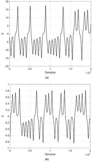
Figure 2. Lorenz chaotic time series solving (7) using a fourth-order Runge–Kutta, with $h=0.0001$ and initial conditions $(x_0,y_0,z_0)=(0.1;0.1;0.1)$. (a) Original, (b) Scaled.

The scaled Lorenz system is described in (9), where $k_1=k_2=k_3=20$, and Figure 2b shows the behavior of the scaled chaotic time series.

$$\begin{array}{c}\dot{u}=\sigma (\frac{k_2}{k_1}v-u)\hfill \\ \dot{v}=\frac{k_1}{k_2}u(\rho -k_{3}w)-v\hfill \\ \dot{w}=\frac{k_1{k}_2}{k_3}uv-\beta w\hfill \end{array}$$

(9)

3.2. Hindmarsh–Rose Neuron

The HRN model represents snail neurons obtained by voltage-clamp experiments. It is simple and easy to implement and can effectively simulate a molluscum neuron’s repetitive and irregular behavior. It also has many neuronal behavioral characteristics such as periodic peak discharge, periodic cluster discharge, chaotic peak discharge, and chaotic cluster discharge [35]. The HRN model is given in (10) [28], where x is the neuronal membrane voltage, y is the recovery variable associated with the current in the neuronal cell, z is the slow adaptability current, and the other parameters can have the following values to generate chaotic behavior: $a=0.5$, $b=1$, $a_1=-0.1$, $b_1=-0.045$, $k=0.2$, $\phi =1$, $\epsilon =0.02$, and $s=-1.605$ [28]. Figure 3 shows the chaotic time series of the variable x of the HRN.

$$\begin{array}{c}\dot{x}=-s(-a{x}^3+x^2)-y-bz\hfill \\ \dot{y}=\phi (x^2-y)\hfill \\ \dot{z}=\epsilon (s{a}_{1}x+b_1-kz)\hfill \end{array}$$

(10)

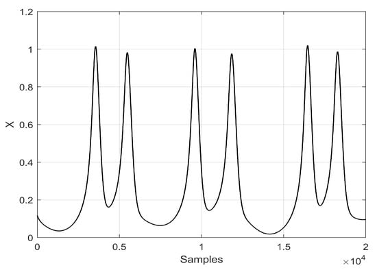
Figure 3. Chaotic time series of variable x of HRN by setting $h=0.01$ and initial conditions $(x_0,y_0,z_0)=(0.1169;0.0356;0.0103)$.

3.3. Decimation of the Chaotic Time Series

To emulate an increase in the prediction horizon, we decided to decimate the time series before conducting the reservoir training, as shown in [18]. The decimation operation by an integer factor $D>1$ on a sequence $\mathbf{x}\left[\mathbf{n}\right]$ consists of keeping every Dth sample of $\left[\mathbf{x}\right(\mathbf{n}\left)\right]$ and removing $D-1$ in-between samples, generating an output sequence $\mathbf{y}\left[\mathbf{d}\right]$ [36]. One can only use this proposal if the main characteristics of the time series do not change, and therefore its Lyapunov exponents and Kaplan–Yorke dimension remain at around the same values without decimation.

This work used the time-series analysis (TISEAN) software to evaluate the Lyapunov exponents from the chaotic time series and the Kaplan–Yorke dimension [37], whose equation is given in (11) and includes the Lyapunov exponents’ values.

$$D_{KY}=k+\frac{{\sum }_{i=1}^{k}L{E}_i}{|L{E}_{k+1}|}$$

(11)

4. Prediction Using ESNs

This section describes the prediction of both chaotic systems, the Lorenz and HRN, using ESNs.

4.1. Lorenz System

The prediction of the Lorenz chaotic time series is performed herein by applying decimation D. Table 1 shows the values of the positive Lyapunov exponent (LE+) and Kaplan–Yorke dimension $\left(D_{KY}\right)$ without decimation (None) and for the three decimation cases with D equal to 10, 25, and 50. The corresponding chaotic time series from this table are shown in Figure 4. As can be seen, the dynamical behavior of the chaotic time series by applying decimation was quite similar to the original data and this helped to increase the prediction horizon, as shown in the remainder of this manuscript.

Table 1. Lyapunov exponent (LE+) and Kaplan–Yorke dimension $\left(D_{KY}\right)$ of the Lorenz system without decimation and for decimation values of 10, 25, and 50.

D	None	10	25	50
LE+	$0.0061$	$0.0016$	$0.0022$	$0.0038$
$D_{KY}$	$2.7995$	$2.2518$	$2.1265$	$2.1079$

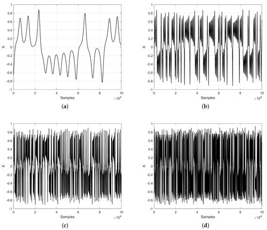
Figure 4. Chaotic time series of Lorenz system: (a) without decimation $D=0$, and with (b) $D=10$, (c) $D=25$, and (d) $D=50$.

For the selection of the ESN hyperparameters to predict the time series of the Lorenz system, we used the grid search method, varying the leaking rate and spectral radius, with 100 neurons $(N=100)$ in the reservoir. According to the recommendation mentioned in Section 2.1, there should be between 1000 and 5000 neurons for a training dataset of 10,000 points; however, we sought to increase the prediction horizon with the least number of neurons possible. The matrices $\mathbf{W}$ and ${\mathbf{W}}_{\mathbf{in}}$ were randomly generated from a range of $[-1,1]$, and $\mathbf{W}$ was re-scaled according to the spectral radius to guarantee the echo state property and fully-connected topology. Figure 5 shows the results of the grid search, where it can be seen that for large values of the leaking rate and spectral radius, the root-mean-squared error (RMSE) tended to increase.

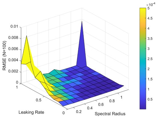
Figure 5. Grid search for the selection of ESN hyperparameters.

The prediction of the chaotic time series was conducted by generating 10,000 data points from the time series to perform the reservoir training, establishing a leaking rate of $0.5$ and a spectral radius of $0.41$, according to the results shown in Figure 5, and finally, a regularization parameter of the ride regression of $1\times {10}^{-8}$. Table 2 shows the results of the prediction for the times series generated from the Lorenz system using reservoir computing with three decimation values. It can be seen that in all the decimation cases, the total prediction steps increased, multiplying the decimation value by the steps ahead. For example, for the case where $D=25$, there was a prediction of 60 steps ahead and a total of 1500 steps ahead. To measure the root mean square error (RMSE) and correlation coefficient (CC), we made several predictions to obtain approximately 5000 points. In all cases, the error values were very close, allowing us to conclude that decimation enabled an increase in the number of predicted steps ahead without significantly changing the RMSE and CC.

Table 2. Results of the chaotic time-series prediction of Lorenz system using ESN with and without the three different decimation values.

D	Steps Ahead	Total Steps Ahead	Steps Predicted	RMSE	CC
None	250	250	5000	$4.6020\times {10}^{-6}$	$0.999960$
10	80	800	5040	$2.3270\times {10}^{-6}$	$0.999992$
25	60	1500	5040	$6.4784\times {10}^{-6}$	$0.999968$
50	30	1500	5010	$1.4494\times {10}^{-6}$	$0.999995$

4.2. Hindmarsh–Rose Neuron

As with the prediction of the chaotic time series for the Lorenz system, a similar process was performed for the HRN. First, the Lyapunov exponents and Kaplan–Yorke dimension were calculated using different decimation values, as shown in Table 3. Figure 6 shows the results of the time series for the four cases listed in Table 3.

Table 3. Lyapunov exponent (LE+) and Kaplan–Yorke dimension $\left(D_{KY}\right)$ of the Hindmarsh–Rose Neuron without decimation and for decimation values of 10, 25, and 50.

D	None	10	25	50
LE+	$0.0012$	$0.0113$	$0.0283$	$0.0566$
$D_{KY}$	$2.3401$	$2.2754$	$2.2748$	$2.2736$

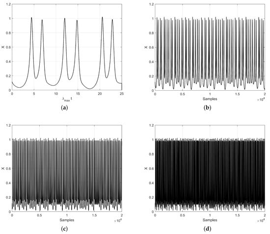
Figure 6. HRN chaotic time series: (a) without decimation, and with decimation (b) $D=10$, (c) $D=25$, and (d) $D=50$.

The next step was to predict the different decimated time series using the ESN. For this, again, we generated 10,000 data points, as with the Lorenz system, to perform the training, setting a leaking rate of $0.5$ and a spectral radius of $0.41$. The matrices $\mathbf{W}$ and ${\mathbf{W}}_{\mathbf{in}}$ were randomly generated and the reservoir comprised 100 neurons. Table 4 shows the obtained results.

Table 4. Prediction results of the HRN chaotic time series shown in Figure 6 and using the ESN with 100 neurons in the hidden layer.

D	Steps Ahead	Total Steps Ahead	Steps Predicted	RMSE	CC
None	350	350	10,150	$4.5872\times {10}^{-5}$	$0.999696$
10	100	1000	10,000	$4.1105\times {10}^{-7}$	$0.999997$
25	45	1125	10,035	$1.5395\times {10}^{-5}$	$0.999898$
50	7	350	10,000	$1.4543\times {10}^{-4}$	$0.999045$

Decimating the HRN time series increased the number of predicted steps ahead. However, when $D=50$, it was impossible to improve the prediction, even though this decimation value did not change the system’s dynamics. This indicates that the maximum decimation value that allows for an increase in the prediction steps depends on each chaotic system.

5. ESN Optimization Using PSO

Metaheuristics are iterative techniques and algorithms that use some level of randomness to discover optimal or near-optimal solutions to computationally hard problems [30]. Among the most commonly applied are differential evolution (DE) [38], genetic algorithms (GA) [39], and PSO [40]. This section shows the application of PSO to enhance time-series prediction [30]. We show the optimization of the ESN applying PSO and considering different decimation cases. The final results of predicting the chaotic time series of the Lorenz system and HRN show the superiority of our technique, allowing predictions of up to 10,000 steps ahead as detailed below.

5.1. Echo State Network Optimization

The ${\mathbf{W}}_{\mathbf{in}}$ and $\mathbf{W}$ matrices were randomly generated. For this reason, we proposed to optimize some of them to increase the prediction horizon. The weight matrix $\mathbf{W}$ of the reservoir must be re-scaled to a sparse matrix with a spectral radius less than or equal to 1 to maintain the echo state property [41]. This condition complicates the optimization of the $\mathbf{W}$ matrix; therefore, we decided to optimize the ${\mathbf{W}}_{\mathbf{in}}$ matrix.

The initial population of the PSO algorithm corresponds to the values of the ${\mathbf{W}}_{\mathbf{in}}$ matrix used in Section 4 to increase the prediction. The fitness function is the RMSE between the target values $\left(y_{target}\right)$ and the predicted values $\left(y_{pred}\right)$ of the chaotic time series. This procedure is performed for the Lorenz system and HRN.

$$RMSE=\sqrt{\frac{1}{T}\sum _{i=1}^T{(y_{target}-y_{pred})}^2}$$

(12)

Figure 7 shows our proposed optimization process to predict the time series of the Lorenz system and the HRN.

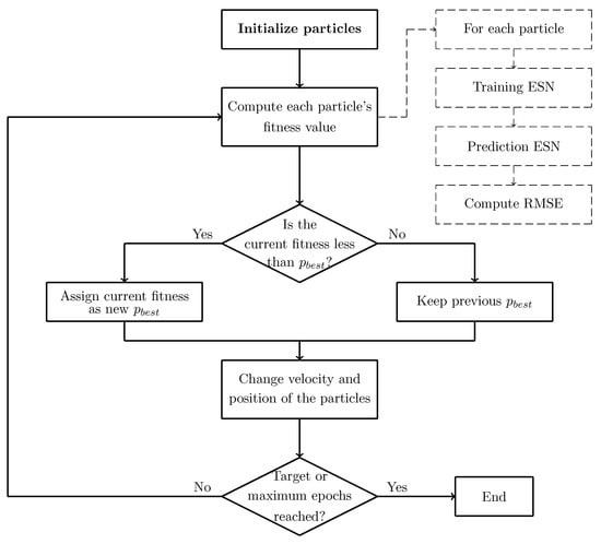
Figure 7. Proposed flow diagram of the ESN optimization process for predicting chaotic time series.

5.2. Enhanced Prediction of Lorenz System Using Optimized ESN

From the optimization process of the ESN, we chose the two most optimistic cases from Table 2, which correspond to the chaotic time series with decimations of 25 and 50. The PSO algorithm was run with a population of 30 particles and 10 generations, and we decided to perform a scaled optimization. For example, when $D=25$, the optimization was performed for 100 steps ahead, the ${\mathbf{W}}_{\mathbf{in}}$ matrix was in the initial population for the subsequent optimization of 150 steps ahead, and so on, until it was impossible to increase the steps ahead with a small error. Table 5 shows the results of the different optimization runs for the two decimations, 25 and 50. Figure 8 shows the prediction results for $D=25$ and Figure 9 for $D=50$. In both cases, one can appreciate that the predicted steps ahead were increased and that the absolute error was low.

Table 5. Optimized ESN for times-series prediction of Lorenz system.

Run	D	Steps Ahead	Total Steps Ahead	Steps Predicted	RMSE
1	25	250	6250	5000	$3.3315\times {10}^{-5}$
2					$7.7769\times {10}^{-6}$
3					$6.1854\times {10}^{-5}$
4					$1.9145\times {10}^{-5}$
5					$1.2868\times {10}^{-5}$
6					$4.6597\times {10}^{-5}$
1	50	200	10,000	5000	$0.5899\times {10}^{-5}$
2					$8.8973\times {10}^{-6}$
3					$3.6936\times {10}^{-5}$
4					$5.1623\times {10}^{-5}$
5					$1.3510\times {10}^{-5}$
6					$7.2846\times {10}^{-5}$

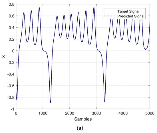
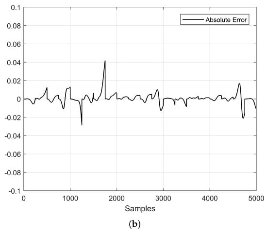
Figure 8. Time-series prediction (Lorenz system) using an optimized ESN with $D=25$. (a) Predicted time series and target signal, and (b) Absolute error.

Figure 9. Time-series prediction (Lorenz system) using an optimized ESN with $D=50$. (a) Predicted time series and target signal, and (b) Absolute error.

5.3. Enhanced Prediction of Hindmarsh–Rose Neuron Using Optimized ESN

For the HRN, we performed the same scaled optimization procedure and selected the cases where $D=10$ and $D=25$, which obtained the best results, as seen in Table 4. Table 6 shows the optimization results.

Table 6. Optimized ESN for times-series prediction of HRN.

Run	D	Steps Ahead	Total Steps Ahead	Steps Predicted	RMSE
1	10	700	7000	5600	$2.5441\times {10}^{-6}$
2					$1.3352\times {10}^{-5}$
3					$6.2291\times {10}^{-6}$
4					$1.2683\times {10}^{-5}$
5					$1.5212\times {10}^{-5}$
6					$3.2412\times {10}^{-6}$
1	25	300	7500	5100	$3.4141\times {10}^{-6}$
2					$3.8000\times {10}^{-6}$
3					$6.8645\times {10}^{-7}$
4					$1.0267\times {10}^{-6}$
5					$1.8325\times {10}^{-6}$
6					$1.3844\times {10}^{-5}$

From Table 6 and Figure 10 and Figure 11, one can conclude that there was not a big difference between the number of total predicted steps ahead and that there was also no significant difference between the absolute error. However, when $D=25$, one can observe more dynamics in the graph despite having a window of 5000 steps.

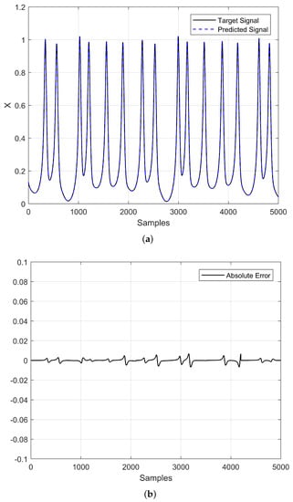
Figure 10. Time-series prediction (HRN) using an optimized ESN with $D=10$. (a) Predicted time series and target signal, and (b) Absolute error.

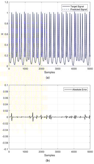
Figure 11. Times series prediction (HRN) using an optimized ESN with $D=25$. (a) Predicted time series and target signal, and (b) Absolute Error.

5.4. Prediction Results and Comparison with Related Works

In this work, we took into account two main objectives; the first was focused on how to increase the prediction steps of chaotic time series and the second was to keep a reservoir with a small size. Table 7 shows the results obtained from the prediction using the optimized ESN with decimation cases for the Lorenz system and HRN, and they were compared with similar works. As one can appreciate, our prediction results were pretty competitive. For example, for the Lorenz system without decimation, the prediction was 250 steps ahead, which was a similar result to that reported in [25], where the authors used three times the number of neurons in the reservoir. In [6], the authors predicted 460 steps using 5000 neurons in the reservoir, which was significantly different from our work in that in all cases, the ESN consisted of only 100 neurons in the reservoir. On the other hand, we can highlight how the decimation process increased the number of predicted steps ahead; only with a decimation of 10 did we improve on the results presented in [42].

Table 7. Prediction results using optimized ESN without/with decimation (D) and comparison with related works.

Method	Lorenz				HRN
	Steps Ahead	RMSE	Neurons	${\mathit{W}}_{\mathit{elem}}$	Steps Ahead	RMSE	Neurons	${\mathit{W}}_{\mathit{elem}}$
ESN	250	$4.6020\times {10}^{-6}$	100	$1\times {10}^4$	350	$4.5872\times {10}^{-5}$	100	$1\times {10}^4$
ESN + D10	800	$2.3270\times {10}^{-6}$	100	$1\times {10}^4$	1000	$4.1105\times {10}^{-7}$	100	$1\times {10}^4$
ESN + D25	1500	$6.4784\times {10}^{-6}$	100	$1\times {10}^4$	1125	$1.5395\times {10}^{-5}$	100	$1\times {10}^4$
ESN + D50	1500	$1.4494\times {10}^{-6}$	100	$1\times {10}^4$	350	$1.4543\times {10}^{-4}$	100	$1\times {10}^4$
ESN + PSO + D10	—	—	—	—	7000	$2.5441\times {10}^{-6}$	100	$1\times {10}^4$
ESN + PSO + D25	6250	$3.3315\times {10}^{-6}$	100	$1\times {10}^4$	7500	$3.4141\times {10}^{-6}$	100	$1\times {10}^4$
ESN + PSO + D50	10,000	$5.8987\times {10}^{-6}$	100	$1\times {10}^4$	—	—	—	—
ESN [25]	300	—	300	$9\times {10}^4$	—	—	—	—
ESN [6]	460	—	5000	$5\times {10}^6$	—	—	—	—
RNN-LSTM [6]	180	—	5000	$5\times {10}^6$	—	—	—	—
ANN [6]	120	—	5000	$5\times {10}^6$	—	—	—	—
ESN [42]	700	—	300	$9\times {10}^4$	—	—	—	—
RESN [20]	500	$0.2238$	200	$4\times {10}^4$	—	—	—	—

Another interesting conclusion is that the optimization of the ${\mathbf{W}}_{\mathbf{in}}$ input matrix resulted in an improvement of more than one order of magnitude in the best case. Finally, to the best of our knowledge, chaotic time-series prediction of neural behavior such as the HRN has not been performed before. This type of neuron has a slow behavior that can complicate the prediction task in long windows of time. One can also use other neuron models such as cellular neural networks [43], the Hopfield neuron [44], and the Huber–Braun neuron [45], as well as other systems related to health modeling [4].

6. Conclusions

This work aimed to increase the prediction horizon of chaotic time series using optimized ESNs, including the decimation of the time series generated from the Lorenz system and HRN. The first contribution was the strategy to decimate the time series. In this case, the HRN presented slow behavior, thus requiring special attention during the generation of time series, since by using a larger step size in the numerical method $\left(h\right)$, the chaos can be diminished and one cannot apply decimation to guarantee a large prediction horizon. In this manner, the prediction results given in Table 7, show that our proposed method for optimizing ESN including decimation greatly increased the predicted steps ahead without affecting the time-series dynamics. The second contribution was the optimization of the ${\mathbf{W}}_{\mathbf{in}}$ input matrix of the ESN, implementing a scaled optimization strategy. The optimization was carried out for a certain number of steps ahead and the resulting optimized matrix was used to initialize the population of the following test, guaranteeing the improvement of the prediction results with more steps ahead. This process was carried out until it was impossible to improve the prediction with an established minimum error value.

Another important conclusion is that our proposed method guaranteed larger prediction horizons with just 100 neurons, which is a very good size reduction of the reservoir compared to similar works and obtained quite competitive prediction results with lower computational costs.

References

- Nadiga, B.T. Reservoir Computing as a Tool for Climate Predictability Studies. J. Adv. Model. Earth Syst. 2021, 13, e2020MS002290. [Google Scholar] [CrossRef]
- Dueben, P.D.; Bauer, P. Challenges and design choices for global weather and climate models based on machine learning. Geosci. Model Dev. 2018, 11, 3999–4009. [Google Scholar] [CrossRef]
- Scher, S. Toward Data-Driven Weather and Climate Forecasting: Approximating a Simple General Circulation Model With Deep Learning. Geophys. Res. Lett. 2018, 45, 12616–12622. [Google Scholar] [CrossRef]
- Shahi, S.; Marcotte, C.D.; Herndon, C.J.; Fenton, F.H.; Shiferaw, Y.; Cherry, E.M. Long-Time Prediction of Arrhythmic Cardiac Action Potentials Using Recurrent Neural Networks and Reservoir Computing. Front. Physiol. 2021, 12, 734178. [Google Scholar] [CrossRef] [PubMed]
- Kim, K.j. Financial time series forecasting using support vector machines. Neurocomputing 2003, 55, 307–319. [Google Scholar] [CrossRef]
- Chattopadhyay, A.; Hassanzadeh, P.; Subramanian, D. Data-driven predictions of a multiscale Lorenz 96 chaotic system using machine-learning methods: Reservoir computing, artificial neural network, and long short-term memory network. Nonlinear Process. Geophys. 2020, 27, 373–389. [Google Scholar] [CrossRef]
- Munir, F.A.; Zia, M.; Mahmood, H. Designing multi-dimensional logistic map with fixed-point finite precision. Nonlinear Dyn. 2019, 97, 2147–2158. [Google Scholar] [CrossRef]
- Valencia-Ponce, M.A.; Tlelo-Cuautle, E.; de la Fraga, L.G. Estimating the Highest Time-Step in Numerical Methods to Enhance the Optimization of Chaotic Oscillators. Mathematics 2021, 9, 1938. [Google Scholar] [CrossRef]
- Pathak, J.; Hunt, B.; Girvan, M.; Lu, Z.; Ott, E. Model-Free Prediction of Large Spatiotemporally Chaotic Systems from Data: A Reservoir Computing Approach. Phys. Rev. Lett. 2018, 120, 024102. [Google Scholar] [CrossRef]
- Thissen, U.; van Brakel, R.; de Weijer, A.P.; Melssen, W.J.; Buydens, L.M.C. Using support vector machines for time series prediction. Chemom. Intell. Lab. Syst. 2003, 69, 35–49. [Google Scholar] [CrossRef]
- Scher, S.; Messori, G. Generalization properties of feed-forward neural networks trained on Lorenz systems. Nonlinear Process. Geophys. 2019, 26, 381–399. [Google Scholar] [CrossRef]
- Amil, P.; Soriano, M.C.; Masoller, C. Machine learning algorithms for predicting the amplitude of chaotic laser pulses. Chaos Interdiscip. J. Nonlinear Sci. 2019, 29, 113111. [Google Scholar] [CrossRef] [PubMed]
- Antonik, P.; Gulina, M.; Pauwels, J.; Massar, S. Using a reservoir computer to learn chaotic attractors, with applications to chaos synchronization and cryptography. Phys. Rev. E 2018, 98, 012215. [Google Scholar] [CrossRef] [PubMed]
- Vlachas, P.R.; Pathak, J.; Hunt, B.R.; Sapsis, T.P.; Girvan, M.; Ott, E.; Koumoutsakos, P. Backpropagation algorithms and Reservoir Computing in Recurrent Neural Networks for the forecasting of complex spatiotemporal dynamics. Neural Netw. 2020, 126, 191–217. [Google Scholar] [CrossRef]
- Lu, Z.; Hunt, B.R.; Ott, E. Attractor reconstruction by machine learning. Chaos Interdiscip. J. Nonlinear Sci. 2018, 28, 061104. [Google Scholar] [CrossRef]
- Arcomano, T.; Szunyogh, I.; Pathak, J.; Wikner, A.; Hunt, B.R.; Ott, E. A Machine Learning-Based Global Atmospheric Forecast Model. Geophys. Res. Lett. 2020, 47, e2020GL087776. [Google Scholar] [CrossRef]
- Tian, Z. Echo state network based on improved fruit fly optimization algorithm for chaotic time series prediction. J. Ambient. Intell. Humaniz. Comput. 2022, 13, 3483–3502. [Google Scholar] [CrossRef]
- Pano-Azucena, A.D.; Tlelo-Cuautle, E.; Ovilla-Martinez, B.; de la Fraga, L.G.; Li, R. Pipeline FPGA-Based Implementations of ANNs for the Prediction of up to 600-Steps-Ahead of Chaotic Time Series. J. Circuits Syst. Comput. 2021, 30, 2150164. [Google Scholar] [CrossRef]
- Pathak, J.; Wikner, A.; Fussell, R.; Chandra, S.; Hunt, B.R.; Girvan, M.; Ott, E. Hybrid forecasting of chaotic processes: Using machine learning in conjunction with a knowledge-based model. Chaos Interdiscip. J. Nonlinear Sci. 2018, 28, 041101. [Google Scholar] [CrossRef]
- Li, D.; Han, M.; Wang, J. Chaotic Time Series Prediction Based on a Novel Robust Echo State Network. IEEE Trans. Neural Netw. Learn. Syst. 2012, 23, 787–799. [Google Scholar] [CrossRef]
- Griffith, A.; Pomerance, A.; Gauthier, D.J. Forecasting chaotic systems with very low connectivity reservoir computers. Chaos Interdiscip. J. Nonlinear Sci. 2019, 29, 123108. [Google Scholar] [CrossRef] [PubMed]
- Racca, A.; Magri, L. Robust Optimization and Validation of Echo State Networks for learning chaotic dynamics. Neural Netw. 2021, 142, 252–268. [Google Scholar] [CrossRef] [PubMed]
- Wang, Z.; Zeng, Y.R.; Wang, S.; Wang, L. Optimizing echo state network with backtracking search optimization algorithm for time series forecasting. Eng. Appl. Artif. Intell. 2019, 81, 117–132. [Google Scholar] [CrossRef]
- Chen, H.C.; Wei, D.Q. Chaotic time series prediction using echo state network based on selective opposition grey wolf optimizer. Nonlinear Dyn. 2021, 104, 3925–3935. [Google Scholar] [CrossRef]
- Pathak, J.; Lu, Z.; Hunt, B.R.; Girvan, M.; Ott, E. Using machine learning to replicate chaotic attractors and calculate Lyapunov exponents from data. Chaos Interdiscip. J. Nonlinear Sci. 2017, 27, 121102. [Google Scholar] [CrossRef] [PubMed]
- Li, X.; Bi, F.; Yang, X.; Bi, X. An Echo State Network with Improved Topology for Time Series Prediction. IEEE Sensors J. 2022, 22, 5869–5878. [Google Scholar] [CrossRef]
- Strogatz, S. Nonlinear Dynamics and Chaos (Studies in Nonlinearity); CRC Press: Boca Raton, FL, USA, 1994. [Google Scholar] [CrossRef]
- Wang, T.; Wang, D.; Wu, K. Chaotic Adaptive Synchronization Control and Application in Chaotic Secure Communication for Industrial Internet of Things. IEEE Access 2018, 6, 8584–8590. [Google Scholar] [CrossRef]
- Jaeger, H. A Tutorial on Training Recurrent Neural Networks, Covering BPPT, RTRL, EKF and the “Echo State Network” Approach; GMD Report 159; German National Research Center for Information Technology: St. Augustin, Germany, 2002; p. 46. [Google Scholar]
- Bala, A.; Ismail, I.; Ibrahim, R.; Sait, S.M. Applications of Metaheuristics in Reservoir Computing Techniques: A Review. IEEE Access 2018, 6, 58012–58029. [Google Scholar] [CrossRef]
- Jaeger, H.; Lukoševičius, M.; Popovici, D.; Siewert, U. Optimization and applications of echo state networks with leaky- integrator neurons. Neural Netw. 2007, 20, 335–352. [Google Scholar] [CrossRef]
- Yildiz, I.B.; Jaeger, H.; Kiebel, S.J. Re-visiting the echo state property. Neural Netw. 2012, 35, 1–9. [Google Scholar] [CrossRef]
- Bai, Q. Analysis of particle swarm optimization algorithm. Comput. Inf. Sci. 2010, 3, 180. [Google Scholar] [CrossRef]
- Shi, Y. Particle swarm optimization. IEEE Connect. 2004, 2, 8–13. [Google Scholar]
- Tsaneva-Atanasova, K.; Osinga, H.M.; Rieß, T.; Sherman, A. Full system bifurcation analysis of endocrine bursting models. J. Theor. Biol. 2010, 264, 1133–1146. [Google Scholar] [CrossRef] [PubMed]
- Dolecek, G.J. Advances in Multirate Systems; Springer: New York, NY, USA, 2017. [Google Scholar]
- Chlouverakis, K.E.; Sprott, J.C. A comparison of correlation and Lyapunov dimensions. Phys. D Nonlinear Phenom. 2005, 200, 156–164. [Google Scholar] [CrossRef]
- Zhang, Y.; Yu, Y.; Liu, D. The Application of modified ESN in chaotic time series prediction. In Proceedings of the 2013 25th Chinese Control and Decision Conference (CCDC), Guiyang, China, 25–27 May 2013; pp. 2213–2218. [Google Scholar] [CrossRef]
- Xu, D.; Lan, J.; Principe, J. Direct adaptive control: An echo state network and genetic algorithm approach. In Proceedings of the 2005 IEEE International Joint Conference on Neural Networks, Montreal, QC, Canada, 31 July–4 August 2005; Volume 3, pp. 1483–1486. [Google Scholar] [CrossRef]
- Chouikhi, N.; Ammar, B.; Rokbani, N.; Alimi, A.M. PSO-based analysis of Echo State Network parameters for time series forecasting. Appl. Soft Comput. 2017, 55, 211–225. [Google Scholar] [CrossRef]
- Yusoff, M.H.; Chrol-Cannon, J.; Jin, Y. Modeling neural plasticity in echo state networks for classification and regression. Inf. Sci. 2016, 364–365, 184–196. [Google Scholar] [CrossRef]
- Bompas, S.; Georgeot, B.; Guéry-Odelin, D. Accuracy of neural networks for the simulation of chaotic dynamics: Precision of training data vs precision of the algorithm. Chaos Interdiscip. J. Nonlinear Sci. 2020, 30, 113118. [Google Scholar] [CrossRef] [PubMed]
- Tlelo-Cuautle, E.; González-Zapata, A.M.; Díaz-Muñoz, J.D.; de la Fraga, L.G.; Cruz-Vega, I. Optimization of fractional-order chaotic cellular neural networks by metaheuristics. Eur. Phys. J. Spec. Top. 2022, 231, 2037–2043. [Google Scholar] [CrossRef]
- Tlelo-Cuautle, E.; Díaz-Muñoz, J.D.; González-Zapata, A.M.; Li, R.; León-Salas, W.D.; Fernández, F.V.; Guillén-Fernández, O.; Cruz-Vega, I. Chaotic Image Encryption Using Hopfield and Hindmarsh–Rose Neurons Implemented on FPGA. Sensors 2020, 20, 1326. [Google Scholar] [CrossRef]
- González-Zapata, A.M.; Tlelo-Cuautle, E.; Cruz-Vega, I.; León-Salas, W.D. Synchronization of chaotic artificial neurons and its application to secure image transmission under MQTT for IoT protocol. Nonlinear Dyn. 2021, 104, 4581–4600. [Google Scholar] [CrossRef]
Publisher’s Note: MDPI stays neutral with regard to jurisdictional claims in published maps and institutional affiliations. |
© 2022 by the authors. Licensee MDPI, Basel, Switzerland. This article is an open access article distributed under the terms and conditions of the Creative Commons Attribution (CC BY) license (https://creativecommons.org/licenses/by/4.0/).