A 2D Multi-Layer Model to Study the External Magnetic Field Generated by a Polymer Exchange Membrane Fuel Cell

Abstract

An original innovative two-dimensional (2D) multi-layer model based on the Maxwell–Fourier method for the diagnosis of a polymer exchange membrane (PEM) fuel cell (FC) stack is presented. It is possible to determine the magnetic field distribution generated around the PEMFC stack from the (non-)homogenous current density distribution inside the PEMFC stack. Analysis of the magnetic field distribution can indicate whether the FC is healthy or faulty. In this way, an explicit, accurate and fast analytical model can allow the health state of an FC to be studied. To evaluate the capacity and the efficiency of the 2D analytical model, the distribution of local quantities (i.e., magnetic vector potential and magnetic field) in a PEMFC stack has been validated with those obtained by the 2D finite-element analysis (FEA). The comparisons demonstrate excellent results both in terms of amplitude and waveform. The validation of this 2D analytical model is essential for the subsequent generation of an inverse model useful for the diagnosis of a PEMFC.

1. Introduction

1.1. Context of the Paper

Currently, the fuel cell (FC) system presents the advantage of combining high-energy efficiency (e.g., FC efficiency about 50% and heat engine efficiency about 32%) and environmental friendliness compared to other more conventional technologies [1]. This presents an interesting combination for conventional power generation systems, especially in stationary and portable FC applications [2,3,4]. Furthermore, a polymer exchange membrane fuel cell (PEMFC), which is the most commonly used FC in transport applications, is an interesting alternative to the internal combustion engine [5].

In order to transform fuel cells in to a mass-market technology, many challenges must be overcome. For that, it is necessary to estimate and comprehend the possible performance of PEMFC in automotive applications as analyzed in [6]. Hydrogen is a promising energy resource. In order to obtain an overview, various studies are based on economics and storage, while recommendations [7] or a critical view can be given on technologies, applications, trends and challenges [8].

The main application of FCs is in the automotive industry. A comprehensive review and research on FC electrical vehicles are presented in [9]. Many topics such as topologies, power electronic converters, energy management methods, technical challenges, marketing and future aspects are discussed.

Some research studies are conducted on the degradation mechanism and impacts on FC degradation with a focus in hybrid transport applications [10]. Similarly, FC diagnosis methods for embedded automotive applications are detailed in [11].

Many factors such as temperature, reactant humidity, partial pressures of feed gases, obstruction of gas diffusion layers, degradation of the membrane electrode assembly (MEA), flow field structure in combination with MEA, etc., could affect the current density distribution and consequently the PEMFC performance [12]. In order to diagnose the PEMFC, an abundance of methods have been developed from physical models [13,14,15] or experimental data information [16]. These can be divided into two categories [17], viz., intrusive and non-intrusive methods. Often, in order to study the (non-)homogeneous current density distribution inside a PEMFC reflecting an FC failure or a healthy FC, intrusive and inflexible methods are applied. Furthermore, the feedback effect of these methods on the measured current density distribution is uncertain. Therefore, a non-destructive control method for the diagnosis, at reasonable costs, will help in PEMFC deployment [18]. Magneto-tomography is one of the most efficient and easiest non-intrusive methods that comprises the mapping of an external magnetic field produced by any electrical device. This measurement technique allows researchers to deduce the current density distribution inside the device [19] by solving an inverse problem [20,21]. In [12], magneto-tomography is for the first time applied to the analysis and diagnosis of a PEMFC stack. The current density distribution can be evaluated by the Biot–Savart law [12,21,22,23,24,25,26,27,28,29,30,31], the varying-network electric circuit [30,31] or the heuristic search method [32,33] where the external magnetic field is determined by

• numerical method [e.g., finite-element analysis (FEA), volume finite method, etc.], viz., (i) two-dimensional (2D) [27,28], or (ii) three-dimensional (3D) [25,26,27,28,32,33];
• and, experimental data from magnetic sensors, viz., (i) uniaxial [22,23,25,26,30,31,33], or (ii) triaxial [12,24,34].

Experimental validations have been realized on

• FC emulator/simulator [25,30,32,35,36];
• single cell [12,22,23,24,27];
• and, real FC stack [24,25,26,30,31,33,34].

Moreover, studies were performed on the external magnetic field determination by imposing the (non-)homogeneous current density distribution inside a PEMFC with 3D numerical [35,36,37] and experimental [35] validations. It is interesting to note that a ferromagnetic circuit placed around a PEMFC emulator permits concentration of the external magnetic field and, consequently, the detection amplification of an FC failure [35]. The actual methods to determine the current density distribution can be globally described as redundant, time-consuming and have variable accuracy.

1.2. Objective of the Paper

In the literature, to the best of the authors’ knowledge, there is no 2D multi-layer model based on the Maxwell–Fourier method for the diagnosis of a PEMFC stack. This method is based on the formal resolution of Maxwell’s magnetostatic equations in Cartesian coordinates $\left(x,y\right)$ by using the separation of variables method, the Fourier’s series and the superposition principle. This purely analytical multi-layer model could give a perfect theoretical study of the magnetic field distribution with a rapid computation time. Moreover, this model could present more precision than the usual methods. Here, the magneto-tomography study is realized on a real bipolar plate of a PEMFC stack (without ferromagnetic circuit placed around the PEMFC stack) in order to diagnose the health state of this one, viz., (i) healthy FC, and (ii) FC failure. As reported in [35,36,37], the developed analytical model will allow the magnetic field distribution generated around the PEMFC to be determined by imposing the (non-)homogeneous current density distribution inside the FC. The reverse study, which is the second step of this scientific work, could then be easily performed on the 2D multi-layer model. However, this is beyond the scope of this paper. To evaluate the efficiency of the proposed analytical model, the distribution of local quantities (i.e., magnetic vector potential and magnetic field) for a healthy FC and an FC failure has been validated with those obtained by the 2D FEA [38]. The comparisons demonstrate excellent results both in terms of amplitude and waveform. The validation of this 2D analytical model is essential for the subsequent generation of an inverse model. This kind of model, which has never been previously developed for FC diagnosis application, must first be validated (e.g., by numerical validation) in order to finally obtain a powerful diagnostic tool of the FC operating mode.

2. Mathematical Development of 2D Multi-Layer Model

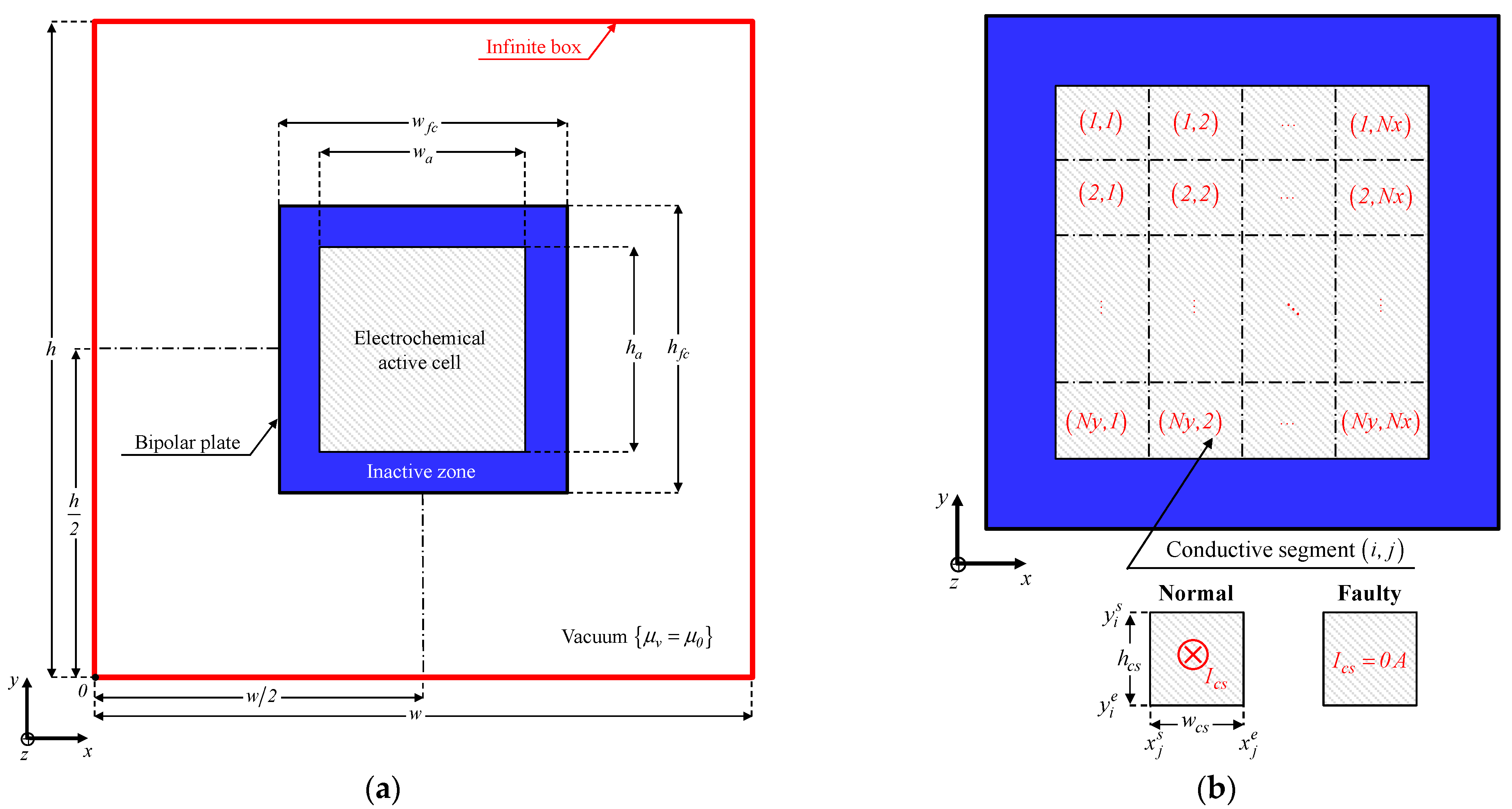
2.1. Problem Description

2.1.1. Bipolar Plate of a PEMFC Stack

Usually, a PEMFC stack (of dimension $w_{fc}\times h_{fc}\times L_{fc}$), with a related constant current of $I_{fc}$, consists of elements in parallel, i.e., compression of two end-plates, two current collectors and several unit cells. Each unit cell is composed of two bipolar plates with an inactive zone (seal) and an electrochemical active cell (of dimension $w_a\times h_a$), two gas diffusion layers and MEA. In electrochemical active cells, at the MEA level, the current density $\mathit{J}=\left\{0; 0; J_z\right\}$, which is perpendicular to the cells with a constant value along the z-axis, is directly related to the flow of hydrogen protons travelling through the electrolyte membrane. Outside of the electrochemical active cell, $\mathit{J}$ is neglected. An FC failure is characterized by a non-homogeneous distribution of $\mathit{J}$ [12]. The considered bipolar plate for the diagnosis of a PEMFC stack, with the geometrical and physical parameters, is illustrated in Figure 1a. This system is surrounded by a vacuum via an infinite box (of dimension $w\times h$).

2.1.2. Normal and Faulty Conductive Segments

To simulate (non-)homogeneous distribution of $\mathit{J}$, this electrochemical active cell of bipolar plates can be decomposed into $Ny\times Nx$ regular conductive segments (of dimension $S_{cs}=w_{cs}\times h_{cs}$ with $w_{cs}=w_a/Nx$ and $h_{cs}=h_a/Nx$), as shown in Figure 1b, where $Ny\in {\mathbb{N}}^{\ast }$ and $Nx\in {\mathbb{N}}^{\ast }$ are the segmentation number in the y- and x-axis, respectively. In Cartesian coordinates $\left(x,y\right)$, the starting and ending points of conductive segments in both axes can be defined by

$$x_j^s=\frac{\left(w-w_a\right)}{2}+\left(j-1\right)·w_{cs} \mathrm{and} x_j^e=x_j^s+w_{cs},$$

(1a)

$$y_i^s=\frac{\left(h+h_a\right)}{2}-\left(i-1\right)·h_{cs} \mathrm{and} y_i^e=y_i^s-h_{cs},$$

(1b)

with $j\in \left\{{\mathbb{N}}^{\ast },Nx\right\}$ and $i\in \left\{{\mathbb{N}}^{\ast },Ny\right\}$.

Any conductive segments $\left(i,j\right)$ may be faulty (not supplied) or normal (supplied). For a non-homogeneous distribution of $\mathit{J}$ reflecting an FC failure, some conductive segments are not supplied (i.e., the current are assumed to be null in the conductive segment). For a homogenous distribution of $\mathit{J}$ reflecting a healthy FC, all conductive segments are supplied by direct current $I_{cs}$ symbolized by $\otimes$ equal to

$$I_{cs}=\frac{I_{fc}}{N_{cs}^n},$$

(2)

with $N_{cs}^n$ the number of conductive segments in a normal condition defined by

$$N_{cs}^n={\displaystyle \sum _{i,j}{M}_{i,j}^{cs}},$$

(3)

where $M_{i,j}^{cs}$ represents the element $\left(i,j\right)$ of the power supply matrix of the conductive segments $M^{cs}$ (of dimension $Ny\times Nx$), viz.,

$$M_{i,j}^{cs}=\{\begin{array}{ll}{\displaystyle 0}& \mathrm{if} \mathbf{faulty} \mathrm{condition},\\ {\displaystyle 1}& \mathrm{if} \mathbf{normal} \mathrm{condition}.\end{array}$$

(4)

2.1.3. Modeling of Spatial Current Density Distribution in any Conductive Segments $\left(i,j\right)$

Figure 2 illustrates the waveform of the spatial distribution of $J_{zij}$ in any conductive segments $\left(i,j\right)$, which can be expressed as a Fourier’s series with $x\in \left[0, w\right]$:

$$J_{zij}={\displaystyle \sum _k{J}_{i,j,k}^{cs}·\sin \left({\beta }_k·x\right)},$$

(5a)

$$J_{i,j,k}^{cs}=\frac{2·J_{\max }^{cs}}{{\beta }_k·w}·F_{i,j,k}^{cs},$$

(5b)

with

$$F_{i,j,k}^{cs}=M_{i,j}^{cs}·\left[\cos \left({\beta }_k·x_j^s\right)-\cos \left({\beta }_k·x_j^e\right)\right]$$

(5c)

where $J_{\max }^{cs}=I_{cs}/S_{cs}$ is the maximum current density in each conductive segment, ${\beta }_k=k\pi /w$ is the spatial frequency (or periodicity) of $J_{zij}$ with $k\in \left\{{\mathbb{N}}^{\ast },K_{\max }\right\}$ the spatial harmonic orders in which $K_{\max }$ is the finite number of spatial harmonics terms.

2.2. List of Assumptions

The 2D magnetic field distribution generated around the PEMFC stack has been studied from multi-layer model by solving Maxwell’s magnetostatic equations in Cartesian coordinates $\left(x,y\right)$. In this analysis, the simplifying assumptions of the analytical model are:

• the end-effects are neglected (i.e., the magnetic variables are independent of z);
• the magnetic vector potential and current density have only one component along the z-axis, i.e., A = {0; 0; A_z} and $J=\left\{0; 0; J_z\right\}$;
• the skin depth effect is not considered;
• many industrial PEMFC stacks use graphite bipolar plates and non-magnetic stainless steels for rods and other mechanical parts [35]. Thus, the absolute magnetic permeability $\mu$ of all components used in bipolar plates of PEMFC stack are very close to the vacuum magnetic permeability ${\mu }_v={\mu }_0=4\pi \times {10}^{-7} H/m$.

2.3. Problem Discretization in Regions

As shown in Figure 3, the bipolar plate for the diagnosis of a PEMFC stack is divided into three regions $\forall x\in \left[0, w\right]$, viz.,

• Vacuum above the electrochemical active cell: Region 1 (R1) for $y\in \left[y_1^s, h\right]$ with ${\mu }_1={\mu }_v={\mu }_0$;
• The electrochemical active cell: Region 2 (R2) for $y\in \left[y_{Ny}^e, y_1^s\right]$, which is divided in the y-axis into sub-regions i (R2_i) for $y\in \left[y_i^e, y_i^s\right]$, with ${\mu }_2={\mu }_v={\mu }_0$;
• Vacuum below the electrochemical active cell: Region 3 (R3) for $y\in \left[0, y_{Ny}^e\right]$ with ${\mu }_3={\mu }_v={\mu }_0$.

2.4. Governing Partial Differential Equations (PDEs) in Cartesian Coordinates

In quasi-stationary, the magnetostatic Maxwell’s equations are represented by Maxwell–Ampère [39]

$$\mathbf{\nabla }\times \mathit{H}=\mathit{J} (\mathit{with} \mathit{J}=0 \mathit{for} \mathit{the} \mathit{no}-\mathit{load} \mathrm{operation}),$$

(6)

Maxwell–Thomson

$$\mathbf{\nabla }·\mathit{B}=0 (\mathit{Magnetic} \mathit{flux} \mathit{conservation}),$$

(7a)

$$\mathit{B}=\mathbf{\nabla }\times \mathit{A} \mathit{with} \mathbf{\nabla }·\mathit{A}=0 (\mathit{Coulomb}’s \mathit{gauge}),$$

(7b)

and the magnetic material equation

$$\mathit{B}=\mu ·\mathit{H}+{\mu }_0·\mathit{M}\mathit{r}$$

(8)

where $\mathit{B}$, $\mathit{H}$ and $\mathit{M}\mathit{r}$ are the magnetic flux density, the magnetic field and the remanent (or residual) magnetization vector (with $\mathit{M}\mathit{r}=0$ for other materials or $\mathit{M}\mathit{r}\ne 0$ for the magnets), respectively.

Using (6)~(8) with the general assumptions of the study, in Cartesian coordinates $\left(x,y\right)$, the general PDEs of magnetostatic in terms of $\mathit{A}=\left\{0; 0; A_z\right\}$ inside an isotropic and uniform material (i.e., $\mu =C^{ste}$) can be expressed by the Laplace’s equation in (R1)

$$\Delta A_{z1}=\frac{{\partial }^2{A}_{z1}}{\partial x^2}+\frac{{\partial }^2{A}_{z1}}{\partial y^2}=0,$$

(9a)

and in (R3)

$$\Delta A_{z3}=\frac{{\partial }^2{A}_{z3}}{\partial x^2}+\frac{{\partial }^2{A}_{z3}}{\partial y^2}=0,$$

(9b)

and the Poisson’s equation in (R2_i)

$$\Delta A_{z{2}_i}=\frac{{\partial }^2{A}_{z{2}_i}}{\partial x^2}+\frac{{\partial }^2{A}_{z{2}_i}}{\partial y^2}=-{\mu }_0·J_{z{2}_i}$$

(9c)

where $J_{z{2}_i}$ is the spatial distribution of $\mathit{J}$ along the x-axis for each i, i.e., in (R2_i), which is defined by

$$J_{z{2}_i}={\displaystyle \sum _j{J}_{zij}}={\displaystyle \sum _k{J}_{i,k}^{cs}·\sin \left({\beta }_k·x\right)},$$

(10a)

$$J_{i,k}^{cs}={\displaystyle \sum _j{J}_{i,j,k}^{cs}}=\frac{2·J_{\max }^{cs}}{{\beta }_k·w}·{\displaystyle \sum _j{F}_{i,j,k}^{cs}}.$$

(10b)

For example, with $Ny\times Nx=2\times 10$ conductive segments, Figure 4 illustrates the waveforms of $J_{z{2}_i}$ for each i in (R2_i) obtained by (10) and for

$$M^{cs}=\left[\begin{array}{cccccccccc}1& 1& 1& 1& 1& 1& 1& 1& 1& 1\\ 1& 0& 1& 1& 1& 0& 0& 1& 0& 1\end{array}\right].$$

(11)

Using (7b), the components of $\mathit{B}=\left\{{\mathit{B}}_x; {\mathit{B}}_y; 0\right\}$ whatever the region can be deduced from $A_z$ by

$$B_x=\frac{\partial A_z}{\partial y} \mathrm{and} B_y=-\frac{\partial A_z}{\partial x}.$$

(12)

From (8), and according to the materials assumptions, the components of $\mathit{H}=\left\{H_x; H_y; 0\right\}$ are defined by $\mathit{H}=\mathit{B}/{\mu }_0$.

2.5. Boundary Conditions (BCs)

In electromagnetic field problems, the general solutions of regions depend on boundary conditions (BCs) at the interface between two surfaces, which are defined by the continuity of parallel magnetic field $H_{\parallel }$ and $A$ [40]. On the infinite box [see Figure 1], $A_z$ satisfies the Dirichlet’s BC, viz., $A_z=0$. Figure 5 represents the respective BCs at the interface between the various regions.

2.6. General Solution of Magnetic Field in Each Region

Using the separation of variables method, the 2D general solution of $A$ in each region can be defined by Fourier’s series. The unknown coefficients (or integration constants) of series are determined analytically from a linear matrix system satisfying the BCs of Figure 5. To simplify the formal resolution of the Cramer’s system, the superposition principle on each sub-region i (R2_i) has been applied.

In (R1) for $y\in \left[y_1^s, h\right]$ and $\forall x\in \left[0, w\right]$, the magnetic vector potential $A_{z1}$, which is a solution of (9a) satisfying the various BCs, is defined by

$$A_{z1}={\displaystyle \sum _{i,k}{\mu }_0·\frac{J_{i,k}^{cs}}{{\beta }_k{}^2}·D{1}_{i,k}·f{1}_{i,k}\left(y\right)·\sin \left({\beta }_k·x\right)}$$

(13)

and the components of ${\mathit{H}}_1$ (i.e., $H_{x1}$ and $H_{y1}$) by

$$H_{x1}=-{\displaystyle \sum _{i,k}\frac{J_{i,k}^{cs}}{{\beta }_k}·D{1}_{i,k}·g{1}_{i,k}\left(y\right)·\sin \left({\beta }_k·x\right)},$$

(14a)

$$H_{y1}=-{\displaystyle \sum _{i,k}\frac{J_{i,k}^{cs}}{{\beta }_k}·D{1}_{i,k}·f{1}_{i,k}\left(y\right)·\cos \left({\beta }_k·x\right)},$$

(14b)

where

$$f{1}_{i,k}\left(y\right)=sh\left[{\beta }_k·\left(h-y\right)\right]/sh\left[{\beta }_k·\left(h-y_i^s\right)\right],$$

(15)

$$g{1}_{i,k}\left(y\right)=ch\left[{\beta }_k·\left(h-y\right)\right]/sh\left[{\beta }_k·\left(h-y_i^s\right)\right],$$

(16)

$$D{1}_{i,k}=NumD{1}_{i,k}/De{n}_{i,k},$$

(17)

with

$$De{n}_{i,k}=a{1}_k·\left(a{3}_{i,k}-a{4}_{i,k}\right)+a{3}_{i,k}·a{4}_{i,k}·\left(a{1}_k{}^2+a{2}_k{}^2\right)-1,$$

(18)

$$NumD{1}_{i,k}=-\left(a{2}_k+a{1}_k·a{4}_{i,k}+1\right),$$

(19)

in which

$$a{1}_k=-sh\left({\beta }_k·h_{cs}\right)/ch\left({\beta }_k·h_{cs}\right),$$

(20)

$$a{2}_k=-1/ch\left({\beta }_k·h_{cs}\right),$$

(21)

$$a{3}_{i,k}=ch\left[{\beta }_k·\left(h-y_i^s\right)\right]/sh\left[{\beta }_k·\left(h-y_i^s\right)\right],$$

(22)

$$a{4}_{i,k}=-sh\left({\beta }_k·y_i^e\right)/ch\left({\beta }_k·y_i^e\right).$$

(23)

In (R3) for $y\in \left[0, y_{Ny}^e\right]$ and $\forall x\in \left[0, w\right]$, the magnetic vector potential $A_{z3}$, which is a solution of (9b) satisfying the various BCs, is defined by

$$A_{z3}=\sum _{i,k}{\mu }_0·\frac{J_{i,k}^{cs}}{{\beta }_k{}^2}·D{3}_{i,k}·f{3}_{i,k}\left(y\right)·\sin \left({\beta }_k·x\right)$$

(24)

and the components of ${\mathit{H}}_3$ (i.e., $H_{x3}$ and $H_{y3}$) by

$$H_{x3}={\displaystyle \sum _{i,k}\frac{J_{i,k}^{cs}}{{\beta }_k}·D{3}_{i,k}·g{3}_{i,k}\left(y\right)·\sin \left({\beta }_k·x\right)},$$

(25a)

$$H_{y3}=-{\displaystyle \sum _{i,k}\frac{J_{i,k}^{cs}}{{\beta }_k}·D{3}_{i,k}·f{3}_{i,k}\left(y\right)·\cos \left({\beta }_k·x\right)},$$

(25b)

where

$$f{3}_{i,k}\left(y\right)=sh\left({\beta }_k·y\right)/ch\left({\beta }_k·y_i^e\right),$$

(26)

$$g{3}_{i,k}\left(y\right)=ch\left({\beta }_k·y\right)/ch\left({\beta }_k·y_i^e\right),$$

(27)

$$D{3}_{i,k}=NumD{3}_{i,k}/De{n}_{i,k},$$

(28)

with

$$NumD{3}_{i,k}=-\left[a{3}_{i,k}·\left(a{1}_k{}^2+a{2}_k{}^2\right)+a{3}_{i,k}·a{2}_k-a{1}_k\right].$$

(29)

In (R2_i) for $y\in \left[y_i^e, y_i^s\right]$ and $\forall x\in \left[0, w\right]$, the magnetic vector potential $A_{z{2}_i}$, which is a solution of (9c) satisfying the various BCs, is defined by

$$A_{z{2}_i}={\displaystyle \sum _k\left\{{\displaystyle \sum _{n=1}^{i-1}{\mu }_0·\frac{J_{n,k}^{cs}}{{\beta }_k{}^2}·D{3}_{n,k}·f{3}_{n,k}\left(y\right)}+{\mu }_0·\frac{J_{i,k}^{cs}}{{\beta }_k{}^2}·\left[\begin{array}{l}C{2}_{i,k}·f2c_{i,k}\left(y\right)\\ \cdots +D{2}_{i,k}·f2d_{i,k}\left(y\right)\\ \cdots +1\end{array}\right]+{\displaystyle \sum _{v=i+1}^{Ny}{\mu }_0·\frac{J_{v,k}^{cs}}{{\beta }_k{}^2}·D{1}_{v,k}·f{1}_{v,k}\left(y\right)}\right\}·\sin \left({\beta }_k·x\right)}$$

(30)

and the components of ${\mathit{H}}_{2_i}$ (i.e., $H_{x{2}_i}$ and $H_{y{2}_i}$) by

$$H_{x{2}_i}={\displaystyle \sum _k\left\{{\displaystyle \sum _{n=1}^{i-1}\frac{J_{n,k}^{cs}}{{\beta }_k}·D{3}_{n,k}·g{3}_{n,k}\left(y\right)}+\frac{J_{i,k}^{cs}}{{\beta }_k}·\left[\begin{array}{l}C{2}_{i,k}·g2c_{i,k}\left(y\right)\\ \cdots -D{2}_{i,k}·g2d_{i,k}\left(y\right)\end{array}\right]-{\displaystyle \sum _{v=i+1}^{Ny}\frac{J_{v,k}^{cs}}{{\beta }_k}·D{1}_{v,k}·g{1}_{v,k}\left(y\right)}\right\}·\sin \left({\beta }_k·x\right)},$$

(31a)

$$H_{y{2}_i}=-{\displaystyle \sum _k\left\{{\displaystyle \sum _{n=1}^{i-1}\frac{J_{n,k}^{cs}}{{\beta }_k}·D{3}_{n,k}·f{3}_{n,k}\left(y\right)}-\frac{J_{i,k}^{cs}}{{\beta }_k}·\left[\begin{array}{l}C{2}_{i,k}·f2c_{i,k}\left(y\right)\\ \cdots +D{2}_{i,k}·f2d_{i,k}\left(y\right)\\ \cdots +1\end{array}\right]+{\displaystyle \sum _{v=i+1}^{Ny}\frac{J_{v,k}^{cs}}{{\beta }_k}·D{1}_{v,k}·f{1}_{v,k}\left(y\right)}\right\}·\cos \left({\beta }_k·x\right)},$$

(31b)

where

$$f2c_{i,k}\left(y\right)=sh\left[{\beta }_k·\left(y-y_i^e\right)\right]/ch\left({\beta }_k·h_{cs}\right),$$

(32)

$$f2d_{i,k}\left(y\right)=ch\left[{\beta }_k·\left(y_i^s-y\right)\right]/ch\left({\beta }_k·h_{cs}\right),$$

(33)

$$g2c_{i,k}\left(y\right)=ch\left[{\beta }_k·\left(y-y_i^e\right)\right]/ch\left({\beta }_k·h_{cs}\right),$$

(34)

$$g2d_{i,k}\left(y\right)=sh\left[{\beta }_k·\left(y_i^s-y\right)\right]/ch\left({\beta }_k·h_{cs}\right),$$

(35)

$$C{2}_{i,k}=NumC{2}_{i,k}/De{n}_{i,k},$$

(36)

$$D{2}_{i,k}=NumD{2}_{i,k}/De{n}_{i,k},$$

(37)

with

$$NumC{2}_{i,k}=a{3}_{i,k}·\left(a{2}_k+a{1}_k·a{4}_{i,k}+1\right),$$

(38)

$$NumD{2}_{i,k}=\left(a{2}_k·a{3}_{i,k}·a{4}_{i,k}-a{1}_k·a{3}_{i,k}+1\right).$$

(39)

3. Comparison of Analytical and Numerical Calculations

3.1. Problem Description

The real bipolar plate of a PEMFC stack is illustrated in Figure 6. The electrochemical active cell is presented with the oxygen/hydrogen channels and surrounded by an inactive zone (seal). The geometrical and physical parameters of the PEMFC stack are reported in

Table 1. Geometrical and physical parameters of a PEMFC stack.

Symbol	Quantity	Values
$S_{fc}=w_{fc}\times h_{fc}$	FC surface	14 × 14 = 196 cm2
S = w × h	Infinite box surface	42 × 42 = 1764 cm2
$S_a=w_a\times h_a$	Electrochemical active cell surface	10 × 10 = 100 cm2
$Ny\times Nx$	Number of conductive segments	25 × 20 = 500
$S_{cs}=w_{cs}\times h_{cs}$	Conductive segment surface	5 × 4 = 20 mm2
$L_{fc}$	FC depth	10 cm

.

To simulate the (non-)homogeneous distribution of $\mathit{J}$, this electrochemical active cell is decomposed into $Ny\times Nx$ regular conductive segments. For example, the discretization with $Ny\times Nx=25\times 20=500$ conductive segments is considered. This discretization of the electrochemical active cell to study health of the FC is illustrated in Figure 7.

Such an important discretization is necessary due to the channels’ size (viz., ~0.8 mm) as shown in Figure 6. The total current flowing through the PEMFC stack (of surface $S_{fc}=$196 cm²) is considered constant and equal to $I_{fc}=$70 A. With an electrochemical active cell surface of $S_a=$100 cm², for a healthy FC [see Figure 7a], this corresponds to $J_{\max }^{cs}=$0.7 A/cm². An example of an FC failure, which can be a consequence of different operating problems, is exposed in Figure 7b. Considering 500 initial conductive segments, 144 segments are faulty (i.e., $J_{\max }^{cs}=$0 A/cm²), so 356 conductive segments present a current density of $J_{\max }^{cs}=$0.983 A/cm².

To evaluate the capacity and the efficacy of the 2D analytical model, the two operating conditions (i.e., normal and faulty condition) are simulated and compared to 2D FEA. The geometrical and physical parameters described previously are simulated on FEMM software [38]. The FE calculations are performed with the same assumptions as the analytical model [see Section 2.2]. The infinite box surface has been imposed to $S=3·S_{fc}=$1764 cm² (viz., $w=3·w_{fc}$ and $h=3·h_{fc}$) so that the equipotential lines of $A_z$ would not be perturbed by the Dirichlet’s CB imposed on the edges. Figure 8 presents the mesh of the system (viz., 107,385 nodes) and different paths with their dimensions added around the PEMFC stack (in red, rated from A to D) in order to evaluate the magnetic field distribution. In this comparison, the analytical solution of $\mathit{A}$ and $\mathit{H}$ in each region have been computed with $K_{\max }=$100.

3.2. Analysis of Equipotential Lines

3.2.1. Healthy FC

The 2D multi-layer model is implemented in order to obtain values of $A_z$ in the bipolar plate for the diagnosis of a PEMFC stack. Figure 9 presents the equipotential lines ($\approx$30 lines) of $A_z$ (or vector plot of $\mathit{H}$) for a healthy FC with the 2D analytical model and 2D FEA. As can be seen, a perfect accuracy between analytical and numerical results allows a first validation of the multi-layer model based on the Maxwell–Fourier method. Due to the homogenous distribution of $\mathit{J}$, and for a square FC, the field lines are symmetrical and circular along the centre of the bipolar plate.

3.2.2. FC Failure

With a non-homogeneous distribution of $\mathit{J}$ reflecting an FC failure, the generated magnetic field is impacted. In Figure 10, the deformation of the equipotential lines of $A_z$ is clearly observed. It is also correctly predicted analytically. On the left, a distortion of the field lines (i.e., asymmetry of field lines) is widely visible due to the presence of a major defect on the right [see Figure 7b].

3.3. Analysis of Magnetic Field Distributions

3.3.1. Healthy FC

Figure 11 represents the distribution of the components of $\mathit{H}=\left\{H_x; H_y; 0\right\}$ for a healthy FC computed by the 2D multi-layer model and verified by the 2D FEA on the various paths. Highly accurate results are achieved between the analytical and numerical model, regardless of the paths and the components of $\mathit{H}=\left\{H_x; H_y; 0\right\}$ in the different regions. It is interesting to note that the waveform and the amplitude of magnetic field components are exactly the same in the four paths (i.e., A to D in Figure 8) independently of the axis.

3.3.2. FC Failure

As for the case of a healthy FC, Figure 12 shows the distribution of the components of $\mathit{H}=\left\{H_x; H_y; 0\right\}$ for an FC failure obtained analytically and numerically on the different paths. Irrespective of the paths and regions, similar and accurate magnetic field results also permit validation of the 2D analytical model. A magnetic field variation reflects a failure in the FC. Around the most damaged part, the greatest decrease in magnetic field is observed (viz., on the path B and C), as shown in Figure 12b,c. As the overall current value $I_{fc}$ is maintained, the current density $J_{\max }^{cs}$ increases in the rest of the FC [see Figure 7]. Thus, the magnetic field variation is less observable for small surface defaults.

4. Conclusions

In this paper, an original innovative 2D multi-layer model, based on the Maxwell–Fourier method, has been developed analytically and validated numerically to estimate the health state of FC. Using magneto-tomography, knowledge of the magnetic field distribution generated around the PEMFC stack allowed for the expression of the (non-) homogeneous current density distribution inside the PEMFC stack and its operation mode. Through FEA validation, the accuracy and efficiency of the analytical model are undeniable.

This 2D analytical model represents the first step towards a comprehensive FC diagnostic tool. For this, the inverse problem of the presented analytical model will have to be solved. From the magnetic field measured around the FC, the inverse model will allow us to know the current density distribution inside the FC. It will then be quick and easy to check the health state of an FC with the advantage of being able to accurately locate a potential fault.

References

1. Dubas, F.; Espanet, C.; Miraoui, A. Design of a high-speed permanent magnet motor for the drive of a fuel cell air compressor. In Proceedings of the IEEE Vehicular Power and Propulsion Conference (VPPC), Chicago, IL, USA, 7–9 September 2005. [Google Scholar] [CrossRef] [Green Version]
2. Hart, D.; Lehner, F.; Jones, S.; Lewis, J. The Fuel Cell Industry Review 2019. E4tech (an ERM Group Company). Available online: http://www.fuelcellindustryreview.com (accessed on 9 January 2020).
3. Wilberforce, T.; Alaswad, A.; Palumbo, A.; Dassisti, M.; Olabi, A.G. Advances in stationary and portable fuel cell applications. Int. J. Hydrogen Energy 2016, 41, 16509–16522. [Google Scholar] [CrossRef] [Green Version]
4. Gurz, M.; Baltacioglu, E.; Hames, Y.; Kaya, K. The meeting of hydrogen and automotive: A review. Int. J. Hydrogen Energy 2017, 42, 23334–23346. [Google Scholar] [CrossRef]
5. Yue, M.; Jemei, S.; Gouriveau, R.; Zerhouni, N. Review on health-conscious energy management strategies for fuel cell hybrid electric vehicles: Degradation models and strategies. Int. J. Hydrogen Energy 2019, 44, 6844–6861. [Google Scholar] [CrossRef]
6. Pahon, E.; Bouquain, D.; Hissel, D.; Rouet, A.; Vacquier, C. Performance analysis of proton exchange membrane fuel cell in automotive applications. J. Power Sources 2021, 510, 230385. [Google Scholar] [CrossRef]
7. Abe, J.O.; Popoola, A.P.I.; Ajenifuja, E.; Popoola, O.M. Hydrogen energy, economy and storage: Review and recommendation. Int. J. Hydrogen Energy 2019, 44, 15072–15086. [Google Scholar] [CrossRef]
8. Yue, M.; Lambert, H.; Pahon, E.; Roche, R.; Jemei, S.; Hissel, D. Hydrogen energy systems: A critical review of technologies, applications, trends and challenges. Renew. Sustain. Energy Rev. 2021, 146, 111180. [Google Scholar] [CrossRef]
9. Inci, M.; Büyük, M.; Demir, M.H.; Ilbey, G. A review and research on fuel cell electric vehicles: Topologies, power electronic converters, energy management methods, technical challenges, marketing and future aspects. Renew. Sustain. Energy Rev. 2020, 137, 110648. [Google Scholar] [CrossRef]
10. Lorenzo, C.; Bouquain, D.; Hibon, S.; Hissel, D. Synthesis of degradation mechanisms and of their impacts on degradation rates on proton-exchange membrane fuel cells and lithium-ion nickel–manganese–cobalt batteries in hybrid transport applications. Reliab. Eng. Syst. Saf. 2021, 212, 107369. [Google Scholar] [CrossRef]
11. Aubry, J.; Steiner, N.Y.; Morando, S.; Zerhouni, N.; Hissel, D. Fuel cell diagnosis methods for embedded automotive applications. Energy Rep. 2022, 8, 6687–6706. [Google Scholar] [CrossRef]
12. Hauer, K.-H.; Potthast, R.; Wüster, T.; Stolten, D. Magnetotomography—A new method for analysing fuel cell performance and quality. J. Power Sources 2005, 143, 67–74. [Google Scholar] [CrossRef]
13. Buchholz, M.; Brebs, V. Dynamic modelling of a polymer electrolyte membrane fuel cell stack by nonlinear system identification. Fuel Cell. 2007, 7, 392–401. [Google Scholar] [CrossRef]
14. Rubio, M.; Urquia, A.; Dormido, S. Diagnosis of performance degradation phenomena in PEM fuel cells. Int. J. Hydrogen Energy 2010, 35, 2586–2590. [Google Scholar] [CrossRef]
15. Chevalier, S.; Trichet, D.; Auvity, B.; Olivier, J.; Josset, C.; Machmoum, M. Multiphysics DC and AC models of a PEMFC for the detection of degraded cell parameters. Int. J. Hydrogen Energy 2013, 38, 11609–11618. [Google Scholar] [CrossRef]
16. Zheng, Z.; Petrone, R.; Péra, M.; Hissel, D.; Becherif, M.; Pianese, C.; Steiner, N.Y.; Sorrentino, M. A review on non-model based diagnosis methodologies for PEM fuel cell stacks and systems. Int. J. Hydrogen Energy 2013, 38, 8914–8926. [Google Scholar] [CrossRef]
17. Geske, M.; Heuer, M.; Heideck, G.; Styczynski, Z.A. Current Density Distribution Mapping in PEM Fuel Cells as An Instrument for Operational Measurements. Energies 2010, 3, 770–783. [Google Scholar] [CrossRef] [Green Version]
18. Pei, P.; Chen, H. Main factors affecting the lifetime of Proton Exchange Membrane fuel cells in vehicle applications: A review. Appl. Energy 2014, 125, 60–75. [Google Scholar] [CrossRef]
19. Ghezzi, L.; Piva, D.; Di Rienzo, L. Current Density Reconstruction in Vacuum Arcs by Inverting Magnetic Field Data. IEEE Trans. Magn. 2012, 48, 2324–2333. [Google Scholar] [CrossRef]
20. Begot, S.; Voisin, E.; Hiebel, P.; Artioukhine, E.; Kauffmann, J.M. D-optimal experimental design applied to a linear magnetostatic inverse problem. IEEE Trans. Magn. 2002, 38, 1065–1068. [Google Scholar] [CrossRef]
21. Potthast, R.; Wannert, M. Uniqueness of Current Reconstructions for Magnetic Tomography in Multilayer Devices. SIAM J. Appl. Math. 2009, 70, 563–578. [Google Scholar] [CrossRef]
22. Izumi, M.; Gotoh, Y.; Yamanaka, T. Verification of Measurement Method of Current Distribution in Polymer Electrolyte Fuel Cells. ECS Trans. 2009, 17, 401–409. [Google Scholar] [CrossRef]
23. Lustfeld, H.; Reißel, M.; Schmidt, U.; Steffen, B. Reconstruction of Electric Currents in a Fuel Cell by Magnetic Field Measurements. J. Fuel Cell Sci. Technol. 2009, 6, 021012. [Google Scholar] [CrossRef]
24. Nasu, T.; Matsushita, Y.; Okano, J.; Okajima, K. Study of Current Distribution in PEMFC Stack Using Magnetic Sensor Probe. J. Int. Counc. Electr. Eng. 2012, 2, 391–396. [Google Scholar] [CrossRef]
25. Le Ny, M.; Chadebec, O.; Cauffet, G.; Dedulle, J.-M.; Bultel, Y.; Rosini, S.; Fourneron, Y.; Kuo-Peng, P. Current Distribution Identification in Fuel Cell Stacks From External Magnetic Field Measurements. IEEE Trans. Magn. 2013, 49, 1925–1928. [Google Scholar] [CrossRef] [Green Version]
26. Le Ny, M.; Chadebec, O.; Cauffet, G.; Rosini, S.; Bultel, Y. PEMFC stack diagnosis based on external magnetic field measurements. J. Appl. Electrochem. 2015, 45, 667–677. [Google Scholar] [CrossRef]
27. Nara, T.; Koike, M.; Ando, S.; Gotoh, Y.; Izumi, M. Estimation of localized current anomalies in polymer electrolyte fuel cells from magnetic flux density measurements. AIP Adv. 2016, 6, 056603. [Google Scholar] [CrossRef] [Green Version]
28. Ifrek, L.; Cauffet, G.; Chadebec, O.; Bultel, Y.; Rouveyre, L.; Rosini, S. 2D and 3D fault basis for fuel cell diagnosis by external magnetic field measurements. Eur. Phys. J. Appl. Phys. 2017, 79, 20901. [Google Scholar] [CrossRef] [Green Version]
29. Claycomb, J.R. Algorithms for the Magnetic Assessment of Proton Exchange Membrane (PEM) Fuel Cells. Res. Nondestruct. Eval. 2017, 29, 167–182. [Google Scholar] [CrossRef]
30. Ifrek, L.; Chadebec, O.; Rosini, S.; Cauffet, G.; Bultel, Y.; Bannwarth, B. Fault Identification on a Fuel Cell by 3-D Current Density Reconstruction From External Magnetic Field Measurements. IEEE Trans. Magn. 2019, 55, 2512271. [Google Scholar] [CrossRef]
31. Ifrek, L.; Rosini, S.; Cauffet, G.; Chadebec, O.; Rouveyre, L.; Bultel, Y. Fault detection for polymer electrolyte membrane fuel cell stack by external magnetic field. Electrochim. Acta 2019, 313, 141–150. [Google Scholar] [CrossRef]
32. Katou, T.; Gotoh, Y.; Takahashi, N.; Izumi, M. Measurement Technique of Distribution of Power Generation Current Using Static Magnetic Field around Polymer Electrolyte Fuel Cell by 3D Inverse Problem FEM. Mater. Trans. 2012, 53, 279–284. [Google Scholar] [CrossRef] [Green Version]
33. Yamanashi, R.; Gotoh, Y.; Izumi, M.; Nara, T. Evaluation of Generation Current inside Membrane Electrode Assembly in Polymer Electrolyte Fuel Cell Using Static Magnetic Field around Fuel Cell. ECS Trans. 2015, 65, 219–226. [Google Scholar] [CrossRef]
34. Akimoto, Y.; Okajima, K.; Uchiyama, Y. Evaluation of Current Distribution in a PEMFC using a Magnetic Sensor Probe. Energy Procedia 2015, 75, 2015–2020. [Google Scholar] [CrossRef] [Green Version]
35. Plait, A.; Giurgea, S.; Hissel, D.; Espanet, C. New magnetic field analyzer device dedicated for polymer electrolyte fuel cells noninvasive diagnostic. Int. J. Hydrogen Energy 2020, 45, 14071–14082. [Google Scholar] [CrossRef]
36. Plait, A.; Dubas, F. Experimental validation of a 2-D multi-layer model for fuel cell diagnosis using magneto-tomography. In Proceedings of the 23rd World Hydrogen Energy Conference (WHEC), Istanbul, Turkey, 26–30 June 2022. [Google Scholar]
37. Lustfeld, H.; Reißel, M.; Steffen, B. Magnetotomography and Electric Currents in a Fuel Cell. Fuel Cells 2009, 9, 474–481. [Google Scholar] [CrossRef]
38. Meeker, D.C. Finite Element Method Magnetics Ver. 4.2. Available online: http://www.femm.info (accessed on 10 October 2018).
39. Stoll, R.L. The Analysis of Eddy Currents; Clarendon Press: Oxfort, UK, 1974. [Google Scholar]
40. Dubas, F.; Boughrara, K. New Scientific Contribution on the 2-D Subdomain Technique in Cartesian Coordinates: Taking into Account of Iron Parts. Math. Comput. Appl. 2017, 22, 17. [Google Scholar] [CrossRef]
Figure 1. (a) Bipolar plate and (b) Electrochemical active cell modeled by N y × N x conductive segments for the diagnosis of a PEMFC stack (see Table 1 for the various parameters).
Mathematics 10 03883 g001
Figure 2. Waveform of the spatial distribution of J z i j in any conductive segments ( i , j ) .
Mathematics 10 03883 g002
Figure 3. Definition of regions in the bipolar plate for the diagnosis of a PEMFC stack.
Mathematics 10 03883 g003
Figure 4. Spatial distribution of: (a) J z 2 1 in (R21), and (b) J z 2 2 in (R22).
Mathematics 10 03883 g004
Figure 5. Boundary conditions at interface between (R1), (R2i) and (R3).
Mathematics 10 03883 g005
Figure 6. Real bipolar plate of a PEMFC stack.
Mathematics 10 03883 g006
Figure 7. FC representation with a discretization of N y × N x = 25 × 20 = 500 conductive segments for: (a) a healthy FC, and (b) an FC failure.
Mathematics 10 03883 g007
Figure 8. The 2D FEA mesh and paths of the magnetic field validation for comparison with { w m ;   h m } = { 5 ;   5 }   m m (see Table 1 for the various parameters).
Mathematics 10 03883 g008
Figure 9. Equipotential lines of A z for a healthy FC obtained by (a) 2D multi-layer model and (b) 2D FEA.
Mathematics 10 03883 g009
Figure 10. Equipotential lines of A z for an FC failure obtained by (a) 2D multi-layer model and (b) 2D FEA.
Mathematics 10 03883 g010
Figure 11. Components of H for a healthy FC calculated by the 2D multi-layer model and verified by 2D FEA on the path: (a) A, (b) B, (c) C and (d) D.
Mathematics 10 03883 g011
Figure 12. Components of H for an FC failure calculated by the 2D multi-layer model and verified by 2D FEA on the path: (a) A, (b) B, (c) C and (d) D.
Mathematics 10 03883 g012aMathematics 10 03883 g012b