Communication Times Reconstruction in a Telecontrolled Client–Server Scheme: An Approach by Kalman Filter Applied to a Proprietary Real-Time Operating System and TCP/IP Protocol

Abstract

Nowadays, various systems were developed in the telecommunications field which make use of technologies for the transmission and reception of information. One of these technologies is the Internet, which was developed in tandem with scientific growth. Therefore, its application in the control of various industrial processes has a notable influence. In this context, there are industrial processes that, due to the potential danger they represent to human beings, must be controlled by means of a remote control system. Such systems can be implemented through client–server communication schemes, which form a network of computers to exchange information. In the exchange of information, delay times are generated. These inactivity times have a close relationship with the latency in the communication network and have a negative impact on the performance of closed-loop control systems. In this sense, for physical implementation, it is essential to measure and mathematically characterize their magnitudes in order to know their variability and thus be able to design control strategies that compensate for their effects. Hence, this research paper presents the reconstruction of the communication times measured from a telecontrol system, where it is assumed that only one subsystem acts as the controller and the other one acts as the controlled. In other words, this paper addresses a control scheme type of single-input-single-output system (SISO). This reconstruction is based on the Kalman filter, which estimates the communication times that are measured on an experimental test bench with a client–server communication scheme. Communication times are characterized as stochastic processes. So, in order to validate the reconstruction presented, the level of dependence between the random processes is evaluated by analyzing their moments of probability as well as their covariance moments. Finally, an analysis based on the mean square error is presented, through which it can be concluded that the reconstruction technique used allows one to know the dynamics of the communication times generated by the remote control process presented in this research.

1. Introduction

The Internet is the primary on-ramp for connecting laptops, handsets, tablets, game consoles, smart televisions, and IoT devices to wired broadband networks [1]. Most of them try to manipulate or telecontrol a physical system remotely. These applications use client–server communication schemes, which, due to the way they are built, require time for processing the information that is sent and received.

These processing times in [2,3] were identified and defined as telecontrol time $T_{Tc,k}$, constituted by the execution times ${\tau }_{c,k}$ and transport times ${\tau }_k$, which in turn are made up of transmission times ${\tau }_{Tx,k}$ and reception times ${\tau }_{Rx,k}$. It should be noted that telecontrol time $T_{Tc,k}$ can present variations because the client–server communication scheme is susceptible to a set of factors. These affect the transport times of the information (reception and transmission), the execution times of the processes, and compromise delivery of the processed information within the maximum deadline time defined by the criteria of H. Nyquist [4] or V. A. Kotélnikov [5], to mention a few. These factors cause fluctuations in the processing time, which could negatively affect the dynamic of the system being telecontrolled. This leads us to the need to formulate mathematical models capable of calculating the increase in resources in the networks of Internet operators to be able to support this increase in the traffic network [6]. Consequently, it “is used” to imitate the behavior of the times involved in the extraction of basic properties, expressed in a set of mathematical attributes.

This is in order to improve the design of network access, maximize the ratio between sent and received information for any pair of source–destination nodes [7], and create efficient traffic control schemes which indirectly reduce transport time on the Internet [8]. In the case of telecontrolled systems, it is possible to improve the system’s behavioral dynamics with the design and development of strategies based onmeasuring the telecontrol time $T_{Tc,k}$.

The behavior of execution times ${\tau }_{c,k}$, fluctuates due to complex modern architecture such as deep pipeline, branch prediction [9], cache sizes [10], the worst-case execution path owing to mutual exclusion [11], and other interactions which cause the non-deterministic behavior of execution times and the asynchrony in the dynamics system [12,13].

Based on the computational complexity theory of [14,15], quantization techniques are used that allow estimating the execution time ${\tau }_{c,k}$ of a computational algorithm. However, it is also possible to find execution times ${\tau }_{c,k}$ reconstruction models, which try to obtain ${\widehat{\tau }}_{c,k}$ at each time instance. These models are based on the auto-regressive moving averages model (ARMA) in which parameters that identify the system were calculated using digital filtering [16,17,18,19,20,21].

In the case of reception times ${\tau }_{Rx,k}$ and transmission times ${\tau }_{Tx,k}$, the variation with respect to time is due to the fact that its duration depends on the increase in technological infrastructure, seasonal or hourly factors, cyclic factors, irregular factors [22], and communications protocols used for the exchange of information [23].

Nowadays, the traffic and control models of communication networks are based on bounded traffic models defined by the ratio of the peak rate and the average rate, and they are effective for the design based on an oversizing ratio, with high data transmission rates and low memory for waiting buffers [8]. In other investigations, mathematical models are proposed that serve to find performance measures of interest such as average delay, variations in delay, arrival time, transmission and reception time (round trip time), occupation in time of the memory in the interconnection circuits, coding times, etc., which mainly form the time existing in the Internet data traffic.

To quantify the encoding, compression, and transmission times of a digital video signal, Ref. [24] presented a model based on autoregressive techniques and Markovian processes. Another way of quantification times is shown in [25], which considers the number of transmitted bits, as well as the type of modulation used. The analysis of traffic data transmission time models for broadband networks based on various protocols was performed in [26]. In the specific case of the TCP protocol, it was mentioned that Poissonian models were used, and they conclude that it is inappropriate for modeling with the mentioned protocol. In the aforementioned manuscripts, the variability of time involved is not considered, but in [8], the authors suggest research based on the application of adaptive signal processing techniques to monitor and predict the performance of a network so that it can make timely and effective control decisions.

The main aim of this manuscript proposal is to show the relevance of a reconstruction technique based on Kalman’s filtering that allows us to describe the behavior of dynamics involved in telecontrol real-time processes. In this specific case of reception time ${\tau }_{Rx,k}$, which, along with transmission time ${\tau }_{Tx,k}$, composes the transport time ${\tau }_k$, a designed and programmed algorithm developed by [2], reported in [3] and applied in [27] as a test bench will be used. The main objective of this algorithm is to determine through computational measurement techniques and the times involved in telecontrol of real-time processes if reconstruction of the behavior is possible using the proposed filter where results could be acceptable to characterize the dynamic of the times involved in Internet communication processes.

The paper organization is as follows: the second section explains the times involved in the remote control process as well as the Kalman filter; the third section presents the development of a test bench used for measuring transmission times in a remote control system, and its statistical characterization and reconstruction from the Kalman filter; the fourth section presents the discussions about the investigation. Finally, the conclusions are presented.

2. Times in Telecontrol Process

The telecontrol system used in this paper is shown in Figure 1. The system is designed to measure and analyze the time involved in the telecontrol process. It is based on the software architecture with a real-time client–server communication scheme developed by [2] and implemented in [27].

The time difference between the controlled variable in a process and the manipulated variable of the control system will be made up of transmission time ${\tau }_{Tx,k}$, reception time ${\tau }_{Rx,k}$, and execution time ${\tau }_{c,k}$. These times will be called communication times $T_{C,k}$ (see (1)).

$$T_{C,k}=\left[\begin{array}{c}{\tau }_{c,k}\\ {\tau }_{Tx,k}\\ {\tau }_{Rx,k}\end{array}\right]$$

(1)

where if the execution time ${\tau }_{c,k}$ in each instance is bounded by the interval (0,$d_k$] with $d_k$ in ${\Re }^{+}$, it is justified that the simulation on the server takes place in real-time. In this context, $d_k$ is the deadline time imposed by the controlled physical system to obtain a punctual response, which does not affect system performance.

The communication scheme can be developed using a Local Area Network (LAN) or a Wide Area Network (WAN), where interconnected devices such as switches and routers can be used. The experiments reported in this paper make exclusive use of a WAN-type network. In fact, in a LAN network, communication is faster, allowing it to communicate in local client–server type schemes. These schemes generate communication times whose amplitude is smaller compared to those obtained when using a WAN.

According to Figure 1, execution time ${\tau }_{c,k}\in {\Re }^{+}$ is the time in which the information is processed on Client A in the interval $k\in Z^{+}$ until processing is completed without considering blockages by reading or writing over communication channels, processor evictions, or other suspensions. Here, it is important to mention that the execution time on the server is not considered because only the server’s external times will be measured.

The reception time ${\tau }_{Rx,k}\in {\Re }^{+}$ is a period of time in which information is sent from Client A to the telecontrol server in an interval $k\in Z^{+}$. The transmission time ${\tau }_{Tx,k}\in {\Re }^{+}$ is the time it takes to send information from the server to remote Client A in an interval $k\in Z^{+}$. Note that in Figure 1, Client B is only used to monitor the output of a simulated system on the server. Telecontrol time in real-time $T_{Tc,k}\in {\Re }^{+}$ is the algebraic sum of execution time ${\tau }_{c,k}$, reception time ${\tau }_{Rx,k}$, and transmission time ${\tau }_{Tx,k}$ in an interval $k\in Z^{+}$. Thus:

$$T_{Tc,k}={\left[\begin{array}{c}1\\ 1\\ 1\end{array}\right]}^T{T}_{C,k}={\tau }_{c,k}+{\tau }_{Tx,k}+{\tau }_{Rx,k}$$

(2)

Model for Reconstruction of the Communication Times in a Telecontrol System

The term “filter” is used to describe an analogically or digitally implemented device that is used to eliminate noise, extract information with smoothing, and predict or reconstruct system behaviors [28]. For the modeling of the times ${\tau }_{c,k}$, ${\tau }_{Tx,k}$, and ${\tau }_{Rx,k}$ in the reviewed literature, the use of digital filtering is reported to estimate or represent their behavior.

The mathematical models that represent the dynamics of the execution time ${\tau }_{c,k}$ are considered fixed [10] or as the worst case of execution times, WCET [11]. However, after conducting a study of the local and global convergence of ${\tau }_{c,k}$ in [16], it was concluded that it can be considered a stochastic system with correlated disturbances, and due to this, it is possible to use an auto-regressive moving average model ARMA (1,1) for the mathematical representation of the execution times ${\tau }_{c,k}$. The system parameters can be obtained by using a digital filter based on the the Instrumental Variable Method IVM [16,18,19] and fuzzy filtering [17,20,21].

The mathematical modeling of transmission and reception times is not a trivial task because they have a behavior that is strongly related to latency in the communication network, and therefore, they have completely random behavior. In this context, they can be modeled by stochastic processes [29] or, failing that, tried in reconstruction techniques for analysis and characterization [30].

A digital filter used as a reconstructor is described in [28,31]. In this context, a reconstructor is a mathematical procedure operating through an observer and correction mechanism (See Figure 2). The algorithm predicts the new state from its previous estimate by adding a correction term proportional to the prediction error, where it is minimized in an optimal sense. Then, for the reconstruction of communication times $T_{C,k}$, the Kalman filter will be used. This will take into account [28,31,32] to propose a model for communication times, considering it as a discrete time system with stochastic behavior and having the general form expressed by Equations (3) and (4).

$$X_{k+1}=A_k{X}_k+B_k{U}_k+V_k$$

(3)

$$T_{C,k}=C_k{X}_k+W_k$$

(4)

where $X_k$ is a states vector, $A_k$ is the system parameter matrix, $B_k$ is the system input matrix coefficient, $U_k$ is the system input vector, $V_k$ is the noise associated with the input system, $T_{C,k}$ is the communication time, $C_k$ is the system outputs coefficient matrix, and $W_k$ is the noise associated with the output system. The prediction of the system’s internal state ${\widehat{G}}_{k+1}$ is defined in (5) as:

$${\widehat{G}}_{k+1}=A_k{\widehat{X}}_k+B_k{U}_k$$

(5)

where ${\widehat{X}}_k$ is expressed in (6):

$${\widehat{X}}_k={\widehat{G}}_k+K_k*(T_{C,k}-C_k{\widehat{G}}_k)$$

(6)

Let $K_k$ be the Kalman K gain defined in (7) by:

$$K_{k+1}=J_{k+1}{C}_{k+1}^T{\left[C_{k+1}{J}_{k+1}{C}_{k+1}^T+R_{k+1}\right]}^{-1}$$

(7)

Such that $J_{k+1}$ is the covariance matrix of states identification and is defined in (8):

$$J_{k+1}=A_k{P}_k{A}_k^T+Q_k$$

(8)

where $Q_k$ is the covariance matrix of noise associated with the input system, which is defined in (9):

$$Q_k=E\left\{V_k{V}_k^T\right\}$$

(9)

Then, $P_{k+1}$ is defined as the covariance matrix of identification error and is given by (10):

$$P_{k+1}=[I-K_{k+1}{C}_{k+1}]J_{k+1}$$

(10)

Here, $R_k$ is the covariance of noise associated with the output system, which is given by (11):

$$R_{k+1}=E\left\{W_{k+1}{W}_{k+1}^T\right\}$$

(11)

Considering the above, the model proposed for the reconstruction of the communication times will be obtained from (4), which is rewritten in (12):

$${\widehat{T}}_{C,k}=C_k{\widehat{X}}_k$$

(12)

where ${\widehat{X}}_k$ is defined as follows:

$${\widehat{X}}_k=\left[\begin{array}{c}{\widehat{\tau }}_{c,k}\\ {\widehat{\tau }}_{Tx,k}\\ {\widehat{\tau }}_{Rx,k}\end{array}\right]$$

(13)

With the following initial conditions of the estimated state vector:

$${\widehat{X}}_0=\left[\begin{array}{c}{\widehat{\tau }}_{c,0}\\ {\widehat{\tau }}_{Tx,0}\\ {\widehat{\tau }}_{Rx,0}\end{array}\right]=\left[\begin{array}{c}0.006\\ 0.9\\ 0.095\end{array}\right]$$

(14)

Then, ${\widehat{T}}_{Tc,k}$ is shown in (15):

$${\widehat{T}}_{Tc,k}={\left[\begin{array}{c}1\\ 1\\ 1\end{array}\right]}^T{\widehat{T}}_{C,k}={\widehat{\tau }}_{c,k}+{\widehat{\tau }}_{Tx,k}+{\widehat{\tau }}_{Rx,k}$$

(15)

3. Results

This section includes the results of this research. The structure of the multi-client–server system that integrates a test bench developed for the study of times involved in the telecontrol process is shown in Figure 1. This served to measure, characterize, and reconstruct the communication times $T_{C,k}$. This is in order to know the dynamics of these non-deterministic times because they determine the occurrence of latency times. In this sense, they can be considered as delays, and these times affect the behavior of the controlled system.

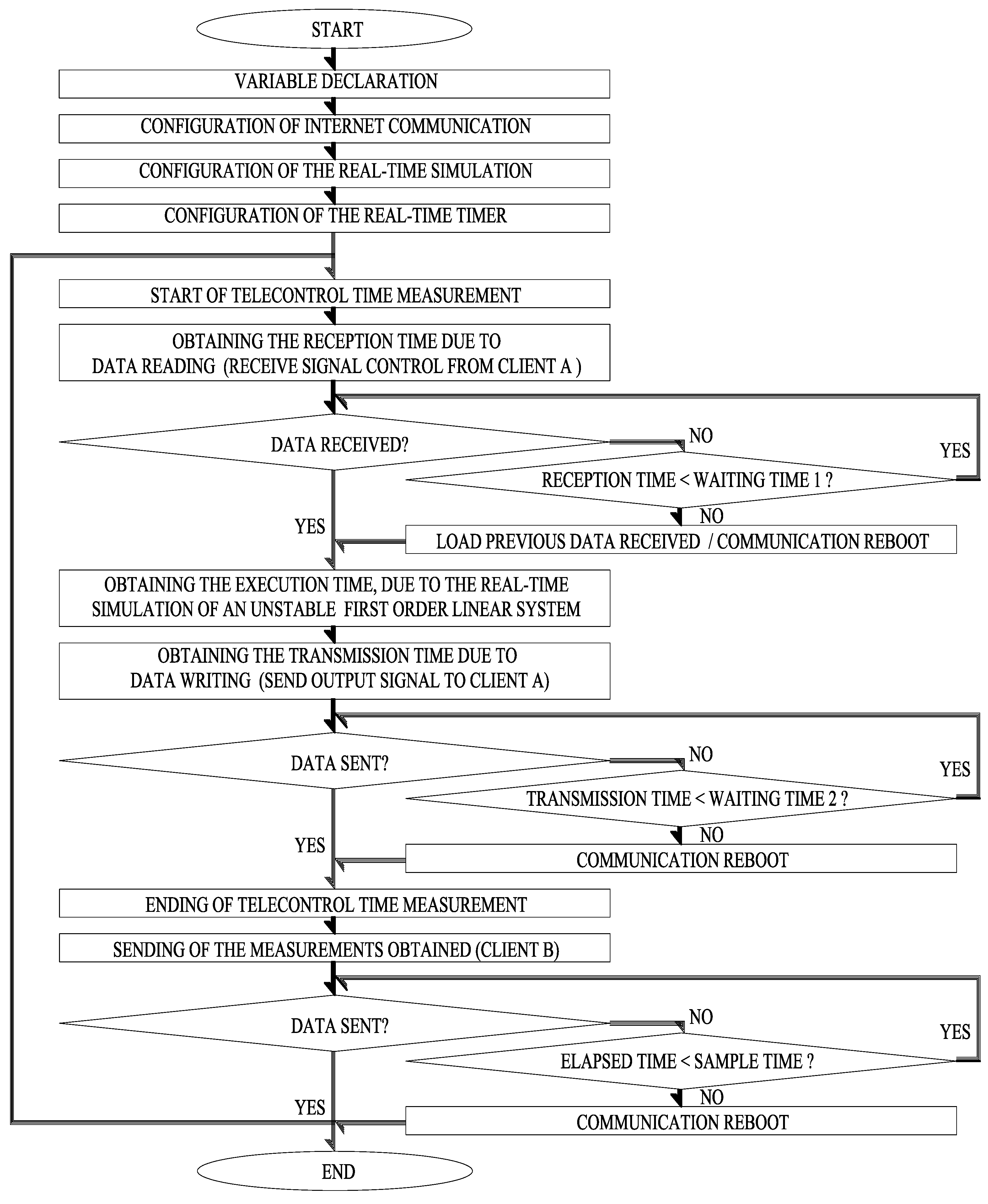
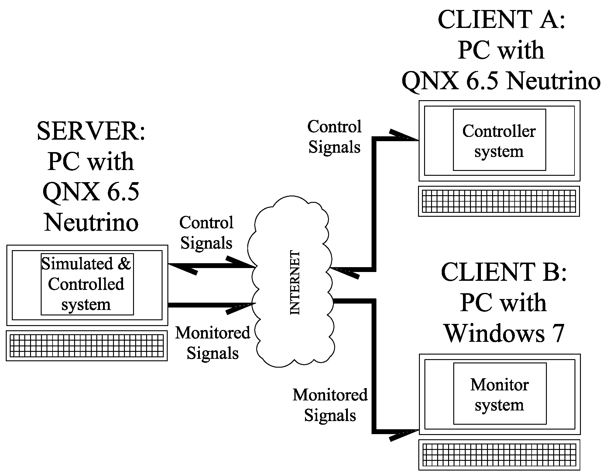
3.1. Telecontrol System Server

To obtain telecontrol times measurement, the software architecture reported in [2,3,30], which is a modular multi-client–server communication scheme, was taken into consideration. The server implementation was performed on a dual processor computer with a speed of 1.6 GigaHertz, 4 Gigabytes of RAM, and the QNX 6.5 Neutrino real-time operating system (RTOS) [33]. The programming was developed in POSIX (Portable Operating System Interface), which is a family of programming standards specified by the IEEE Computer Society and used to maintain software compatibility between UNIX-based operating systems. POSIX defines the Application Programming Interface (API) between command-line and graphical interfaces [34].

The server program executes three main real-time tasks (RTT). The tasks carried out on the server are executed periodically through the use of real-time timers with a sampling period $T=0.1$. Figure 3 shows a user interface flow diagram for the telecontrol server.

The first task realized the communication via Internet to Client A and B using TCP/IP protocol through the use of function socket() from library sys/socket.h [33]. In this paper, this TCP communication protocol was used since it guarantees the reliability and correct order of sent data through a communication socket. The correct data order, verified by the cyclic redundancy check (CRC), avoids loss of information, but it may increase response times. However, it ensures the data accuracy. Therefore, in this paper, this communication protocol was chosen since the implementation of a telecontrol system requires data integrity for its proper performance.

The virtual circuit for transferring information uses network communication ports where information is sent as an 8-byte character string to Client A through the use of network port 7000 (writing socket) and to Client B via network port 7020 (graphing socket), but only information is received from Client A through network port 7010 (reading socket). Network port 7030 was used to send information about measured times of the telecontrol system in real-time.

The second server task is responsible for the simulation of an unstable first-order system, whose transfer function is shown in (16):

$$G\left(s\right)=\frac{\beta }{s+\alpha }$$

(16)

The discrete time recursive model shown in (17) was obtained through the Z-transform:

$$y_k=\frac{\beta }{\alpha }(1-e^{-\alpha T})u_{k-1}+e^{-\alpha T}{y}_{k-1}$$

(17)

where $\beta =1$, $\alpha =-0.5$, $\tau =1/\left|\alpha \right|$ and $T=0.1$. There are real-time applications that use small deadlines (RTT iteration steps) $T_s$, but this is not an indispensable requirement for the implementation of real-time systems (RTS). In this sense, it should be noted that the execution deadline assignment of the real-time tasks that are part of the RTS should be determined based on the speed of change or evolution of the dynamic system, which is determined by its time constant $\tau$. In this context and according to the $\alpha$ parameter defined by the SISO system (16), $\tau =2$, it is proposed to use $T_s=0.1$ as the deadline for the RTT programming. Although this deadline does not represent a challenge for the processing capacity of the RTS, it was determined considering the aforementioned criteria, thus complying with one of the essential characteristics of all RTS [35]. On the other hand, there are communication protocols that, together with the bandwidth of the Internet where these implementations are carried out, guarantee shorter response times.

To avoid preemption times (considered as delays) caused by interaction with other RTT, a high execution priority was assigned by means of the setprio() and getprio() functions of POSIX for QNX RTOS to ensure the minimum existence of preemption tasks due to mutual exclusion. By using this scheduling tool, it is possible to guarantee execution times whose magnitude is lower compared to the scenario in which no priority assignment is made. This action is intended to ensure that the real-time simulation of the unstable system satisfies the deadline associated with the task that simulates it.

The result of the system simulation’s $y_k$ output signal was sent to both clients. Client A used the $y_k$ signal value to obtain the control signal $u_{k-1}$. This value was returned to the server to modify the behavior of the first-order unstable system simulated in real-time. Client B used the output signal to make the comparison between the signal $y_k$ obtained by the real-time control of the first-order unstable system simulation and the ideal output signal.

The third task of the server was programmed to measure the communication times involved in the telecontrol process from the server to client A, within which execution times ${\tau }_{c,k}$, reception times ${\tau }_{Rx,k}$, and transmission times ${\tau }_{Tx,k}$ can be considered. It is worth mentioning that this information was sent to Client B using network port 7030. The measured times can be saved in a database on the server for later analysis, and this activity is considered as the fourth task.

To avoid the appearance of excessive time originated by the reading and writing of information in the communication buffer (latency times), additional secondary real-time tasks were programmed. In this sense, the programming performed for the prevention of such latency times use the select() function from the library sys/select.h of POSIX, with the purpose of implementing blocking type communication sockets. This prevention mechanism was carried out by the first secondary RTT, which has the purpose of assigning a sub-deadline $d_{s1,k}$ for the reception of data by the server. Therefore, if in the current iteration, the reception time ${\tau }_{Rx,k}$ exceeds the sub-deadline $d_{s1,k}$, the server blocks the communication socket and consequently does not wait for the value of the control action $u_{k-1}$ sent by Client A.

In this scenario, to ensure the correct execution of the telecontrol strategy, the server does not consider the control action null. Instead, it considers the value of the control action sent by the Client A in the previous iteration $u_{k-2}$, this being considered for the stabilization of the simulated system in the server. As a consequence of the procedure described above, the server calculates the output of the system $y_k$ to be used in the subsequent iteration and forwards it to Client A. To this end, the other secondary RTT is programmed in the server, which aims at allocating a sub-deadline $d_{s2,k}$. If it is detected that the time of data transmission ${\tau }_{Tx,k}$ exceeds the sub-deadline $d_{s2,k}$, the server blocks the communication socket again, thus terminating the process and preparing to send the information to Client B.

This prevention mechanism helps to limit the sub-deadlines $d_{s1,k}$ and $d_{s2,k}$ as waiting times to ensure that even when the communication times between the server and the clients are of variable magnitude, the deadline $T_S$ (RTT iteration step) is met, such that, if there is a long response time from Client B, and if it exceeds the deadline $T_S$, the communication is terminated to initialize the scheduling loop again. This is repeated until there is confirmed communication with the clients in the control scheme. To guarantee the periodic execution of the main RTTs, a real-time signal timer was programmed to define the sampling period T, such that $T_s$ is less than or equal to T.

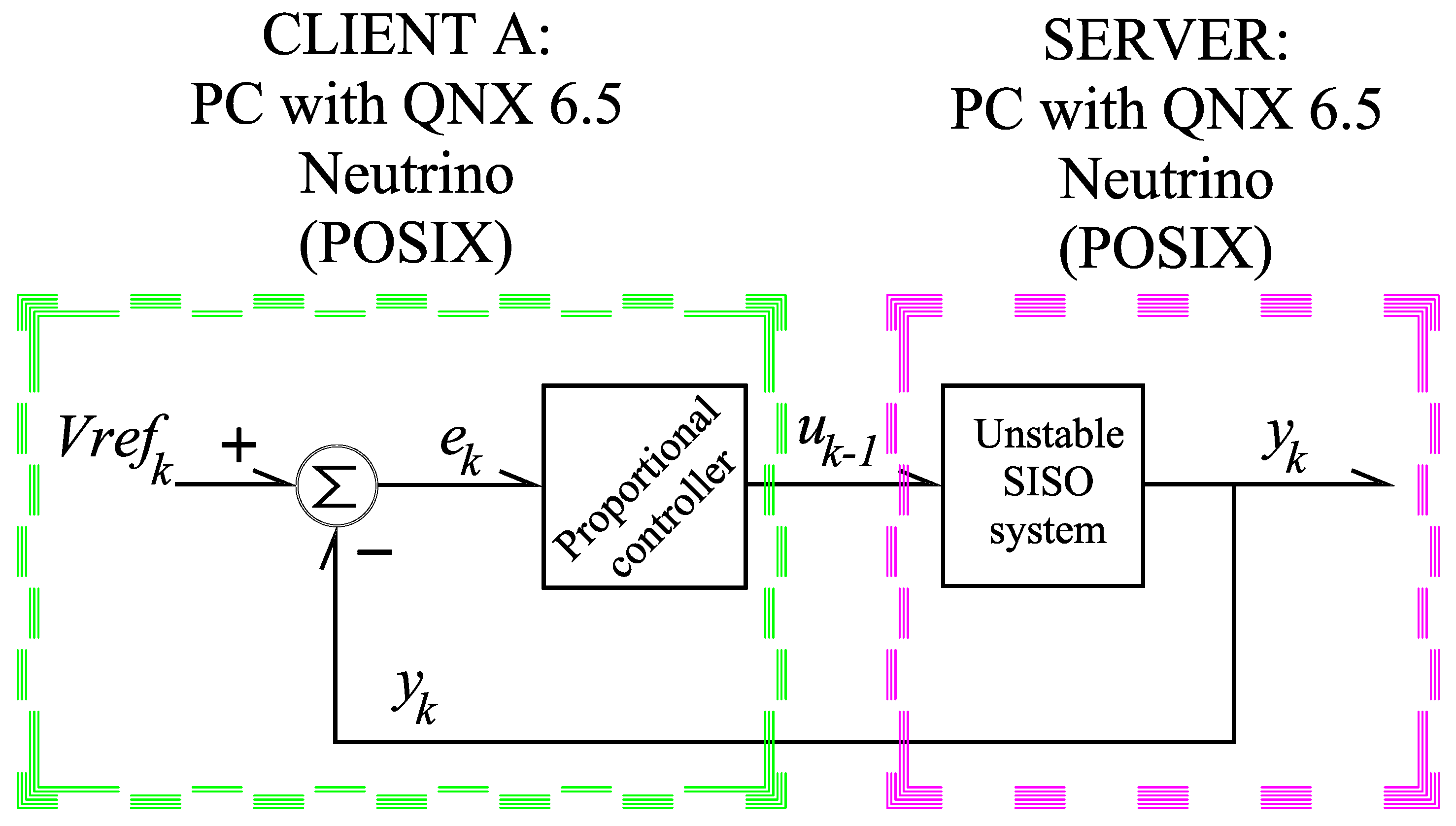
3.2. Client A of the Telecontrol System

Client A was developed on a computer with the QNX 6.5 Neutrino real-time operating system, a dual processor with a speed of 1.6 Gigahertz, and 4 Gigabytes of RAM. The user interface flow diagram for telecontrol Client A is shown in Figure 4.

The three tasks performed by Client A are described as follows: The first task was programmed to communicate with the server to receive information sent on the assigned socket (IP address 201. 163. 201. 153 and network port 7000), which corresponds to the output of the unstable first-order system $y_k$. The second task was used to program and execute a real-time timer. The third task provided a menu where the proportional control scheme designed for the SISO system, denoted by (16), was chosen, assigning a value of $Kp=0.6$, which was tuned by means of the Ziegler–Nichols method from the open loop curve. The block diagram was constructed with its controller in a closed loop (See Figure 5) to observe its behavior and verify that with this gain it has a quick response, maintaining a value of $y_k=6$.

The control signal $u_{k-1}$ will be sent through the network communication port 7010 to the server in order to manipulate or limit the output of the simulated unstable first-order system. As with the server, there is a timing mechanism in the POSIX programming language that allows the control signal to be provided at the indicated times. The timing mechanism provides an iteration step for the programmed task which is equal to the server.

3.3. Client B of the Telecontrol System

Client B (see Figure 6) was implemented in a non-real-time operating system and has the following hardware features: quad-core processor with a processing speed of 3.2 Gigahertz and 8 Gigabytes of RAM. The time-sharing operating system used is Windows, which uses National Instruments industrial development software LABVIEW for the graphic interface development [36].

This is because it offers the possibility of interacting with physical systems through the use of data acquisition cards, as well as monitoring and graphically displaying the information emitted by systems.

The graphical interface is responsible for reading the IP address 201. 163. 201. 153 on network port 7020 and 7030, the information sent by the server. The network port 7020 of this IP address is the socket responsible for sending the value of the output signal of the unstable first-order system to be plotted on the server.

The network port 7030 is the socket responsible for sending values of reception time ${\tau }_{Rx,k}$ and transmission time ${\tau }_{Tx,k}$ measured during communication from the server developed in the QNX 6.5 Neutrino real-time operating system to Client A to be plotted (see Figure 6 communication times). The block diagram of the front panel can be seen in Figure 7.

The information is transported on the Internet by the virtual communication circuit as an 8-byte character string. It is converted to a numerical format and plotted using the developed interface or through the mathematical analysis software MATLAB [37]. These results are shown in Figure 8.

To analyze the effect of the communication times in the simulation of the unstable first-order system, it was added (17) to the code G diagram shown in Figure 7. The proportional control action was also applied to this representation, and its output was compared with the output of the simulated system on the server, which is controlled by Client A.

The variation observed at the beginning of the evolution of the real output signal, which is seen in Figure 6, is due to the use of different timing values in each client. The communication times $T_{C,k}$ were measured by Client A, which, due to their duration and variation, were considered for their graphing, and consequently, their reconstruction. Figure 8 shows the reception and transmission times measured by the server.

Figure 9 shows the execution times measured by Client A. These times are generated due to the calculation of the control action applied to the server.

The times shown in Figure 8 correspond to the transmission and reception of information in the Internet communication scheme, which were measured by the server and vary according to both external and internal factors. With regard to external factors, these may be caused by communication network infrastructure, computer intrusions, latency due to use of the system during peak hours, meteorological phenomena, among others. Therefore, there is no certainty that its variability is known a priori; thus, it is associated with factors that do not depend on the system in real time. Instead, they are due to the latency of the network of communication devices such as access points, routers, hubs, and switches, to mention a few.

Regarding the internal factors associated with the server and Client A, there are pipeline, preemption times due to priority management, exclusion of tasks due to process scheduling effects, and caching, among others. It should be noted that the determination of the deadline for the execution of tasks in real time was made based on the time constant of the dynamic system SISO (14) and not based on the maximum magnitude of the transmission and reception times, since one of the primary characteristics of any RTS is to meet the time constraints imposed by the process or physical phenomenon with which it is interacting.

In this context, it is important to emphasize that server and Client A were both implemented using a real-time operating system. Therefore, only Client B was implemented using a time-sharing operating system. Based on the above, the mechanism to ensure compliance with the deadlines was implemented in the server and Client A to ensure that even when the transmission and reception times have a significant variability (for example, 6 s), the system continues to operate by using the previous value of the control action $u_{k-2}$; thus, these latency times do not compromise the stability of the closed-loop system.

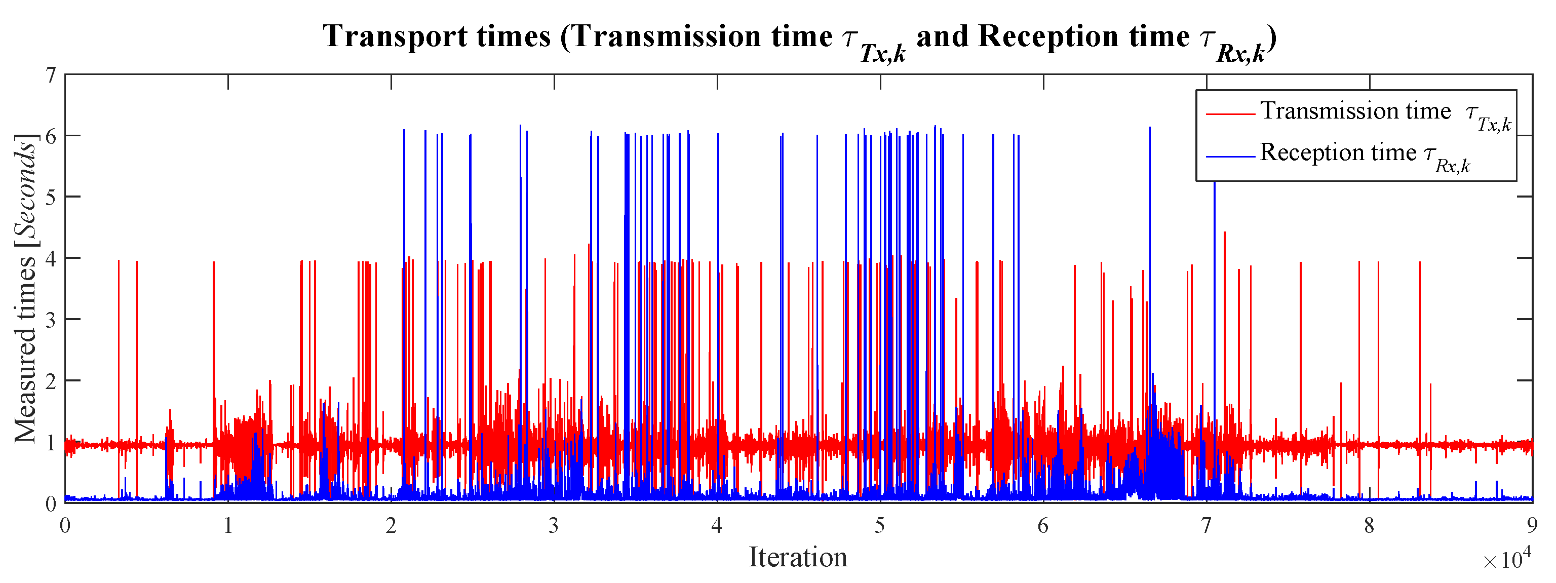
3.4. Characterization of Communication Times $T_{C,k}$ in Telecontrol Systems

To ensure the operating condition of the Kalman filter as a reconstructor of communication times $T_{C,k}$ behavior of a telecontrol system, it is necessary to analyze the temporary covariance of input noise $Q_{T_{C,k}}$ and the covariance of output noise $R_{T_{C,k+1}}$ in execution times ${\tau }_{c,k}$, reception times ${\tau }_{Rx,k}$, and transmission times ${\tau }_{Tx,k}$, to determine its functional dependence using (9) and (11), respectively. $Q_{T_{C,k}}$ is denoted by (18).

$$Q_{T_{C,k}}=\left[\begin{array}{ccc}{Q}_{c,k}& 0& 0\\ 0& Q_{Tx,k}& 0\\ 0& 0& Q_{Rx,k}\end{array}\right]$$

(18)

Figure 10 shows the covariance of associated noises with the system input.

This figure shows $Q_{Tx,k}$, $Q_{Rx,k}$, and $Q_{c,k}$, and it can be observed that at the beginning of system evolution, the behavior of covariance has different values than zero. This allows us to say that at the beginning of reconstruction, the noises associated with the system at input and output have some linear dependence, but as the system evolves, the temporary covariance of the noises associated with the system converges close to zero gradually (See

Table 1. Temporary covariance values of the input noises $Q_{T_{C,k}}$ associated with the system.

${\mathit{Q}}_{\mathit{Tx},\mathit{k}}$	${\mathit{Q}}_{\mathit{Rx},\mathit{k}}$	${\mathit{Q}}_{\mathit{c},\mathit{k}}$
9.59 × 10−12	19.19 × 10−12	3.925 × 10−12

).

$R_{T_{C,k}}$ is represented by (19), and Figure 11 shows the covariance of output noise with the system.

$$R_{T_{C,k}}=\left[\begin{array}{ccc}{R}_{c,k}& 0& 0\\ 0& R_{Tx,k}& 0\\ 0& 0& R_{Rx,k}\end{array}\right]$$

(19)

The same situation is observed in $R_{T_{C,k}}$ (See

Table 2. Temporary covariance values of the output noises $R_{T_{C,k+1}}$ associated with the system.

${\mathit{R}}_{\mathit{Tx},\mathit{k}}$	${\mathit{R}}_{\mathit{Rx},\mathit{k}}$	${\mathit{R}}_{\mathit{c},\mathit{k}}$
4.762 × 10−16	28.57 × 10−16	9.26 × 10−16

). With this, we can ensure that the covariance of input $Q_{T_{C,k}}$ and output $R_{T_{C,k+1}}$ noises have linear independence.

The linear independence allows us to state that the variance of identification error $P_{T_{C,k+1}}$ given in (10) will have the same behavior (Figure 11). Based on the analysis of the values (See

Table 3. Covariance of identification error $P_{T_{C,k+1}}$.

${\mathit{P}}_{\mathit{Tx},\mathit{k}}$	${\mathit{P}}_{\mathit{Rx},\mathit{k}}$	${\mathit{P}}_{\mathit{c},\mathit{k}}$
4.762 × 10−16	28.33 × 10−16	9.293 × 10−16

), we concluded that operating conditions to use the Kalman filter are able to reconstruct the communication times $T_{C,k}$ behavior of a telecontrol real-time system (RTS) and are fulfilled by ensuring that noises associated with the input and output of the system are linearly independent.

When the covariance moment is evaluated by means of a linear type function of two random processes, it is established that a closed interval goes from 0 to 1, where the interval closed on the left denotes independence of the processes and the interval closed on the right denotes a high level of dependence. Therefore, in both cases, it can be observed that at the start of the system evolution, the behavior of the covariance has values different from zero, which means that at the beginning of the reconstruction, the noises associated with the system at the input and output have a certain dependence. However, while the system evolves, the behavior of the temporal covariance of the noises associated with the system tends to a region close to zero. Thus, it can be assured that the noises characterized by the covariance matrices $Q_{Tx,k}$ and $R_{Tx,k+1}$ have linear independence, which allows assurance that the covariance of the identification error will have the same behavior.

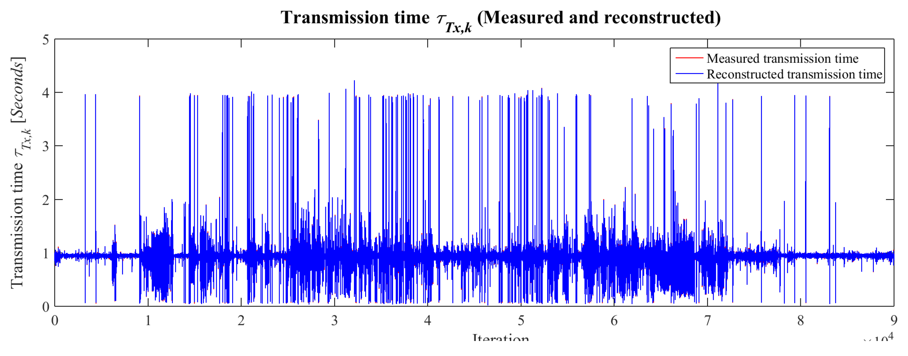
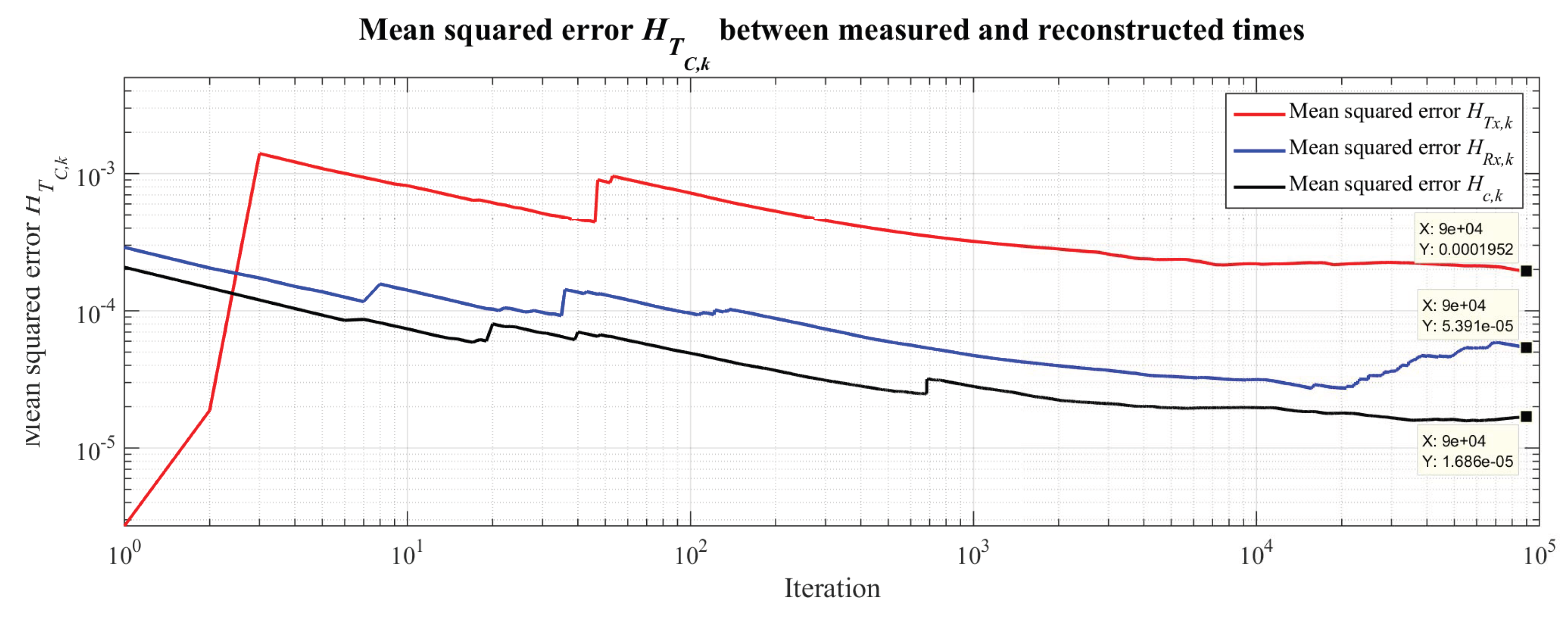
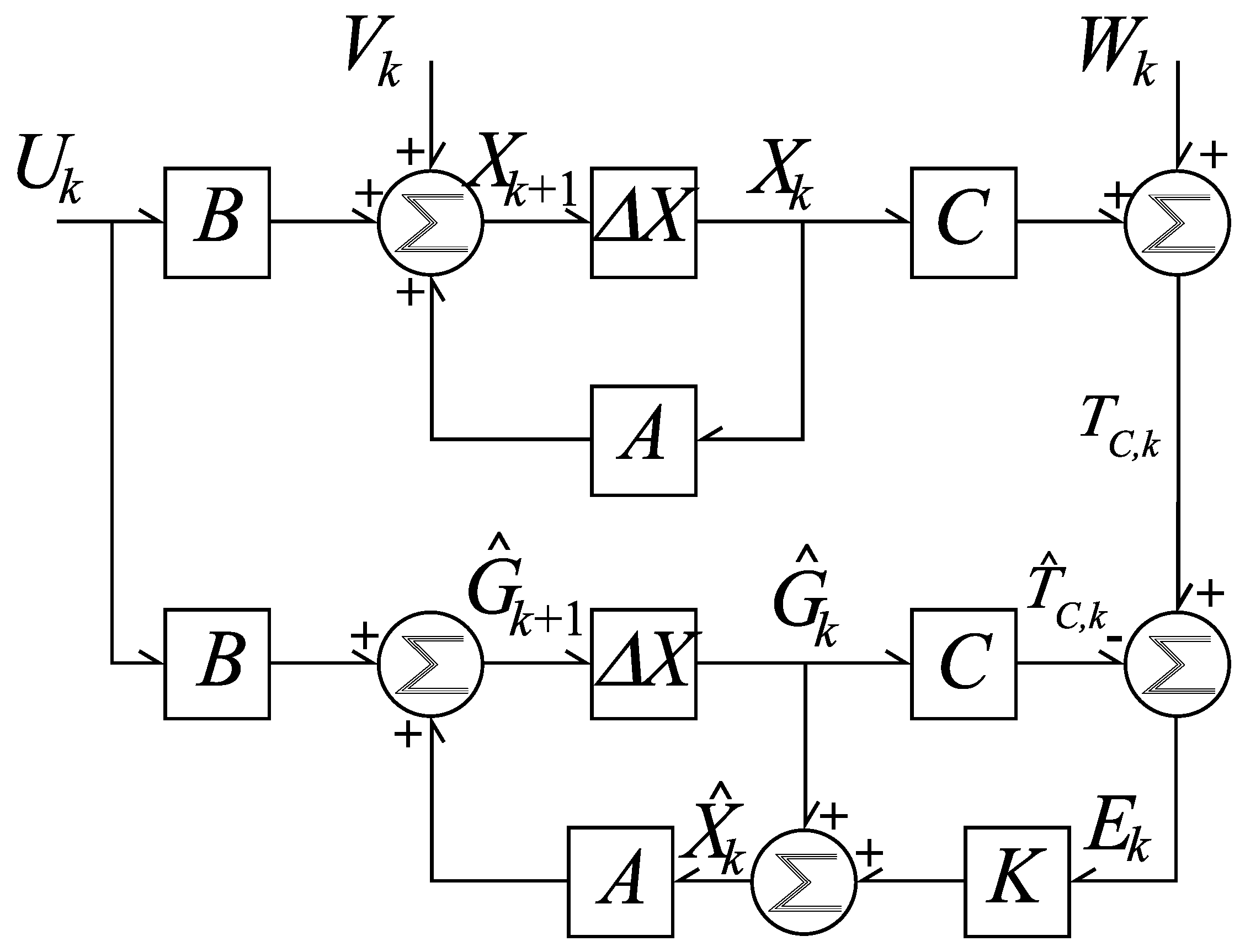
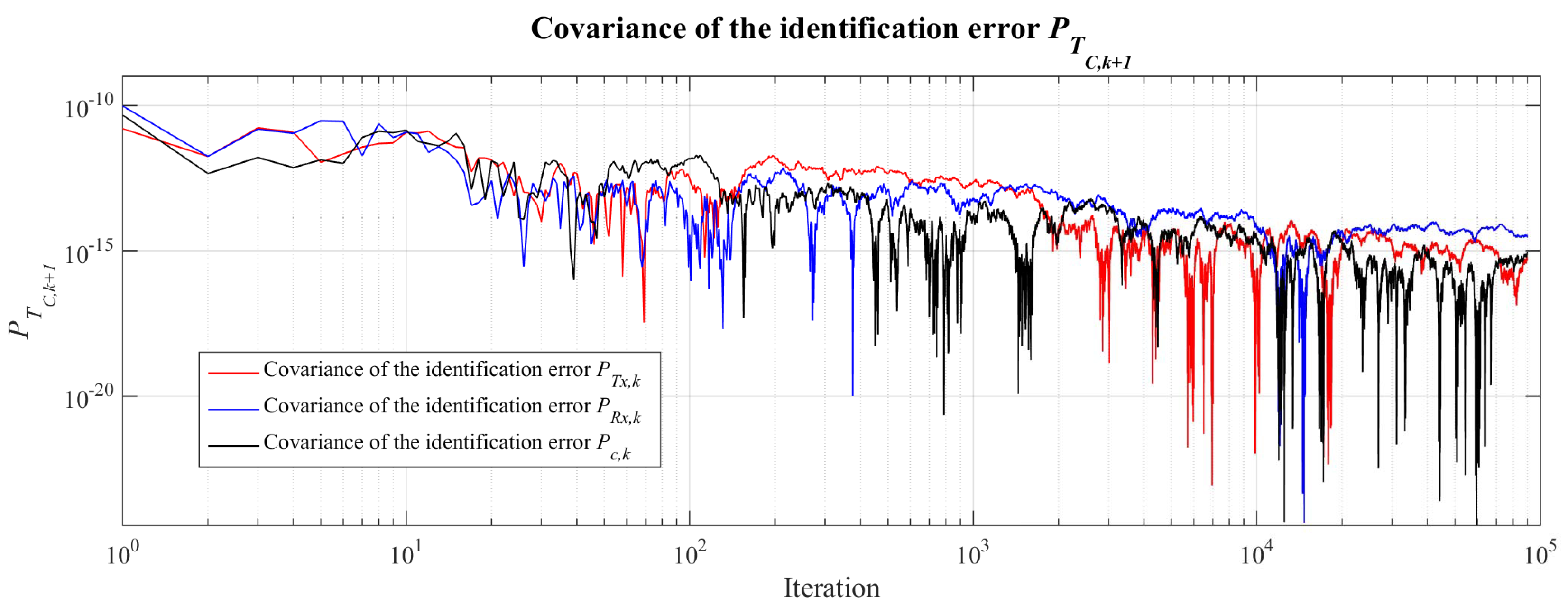
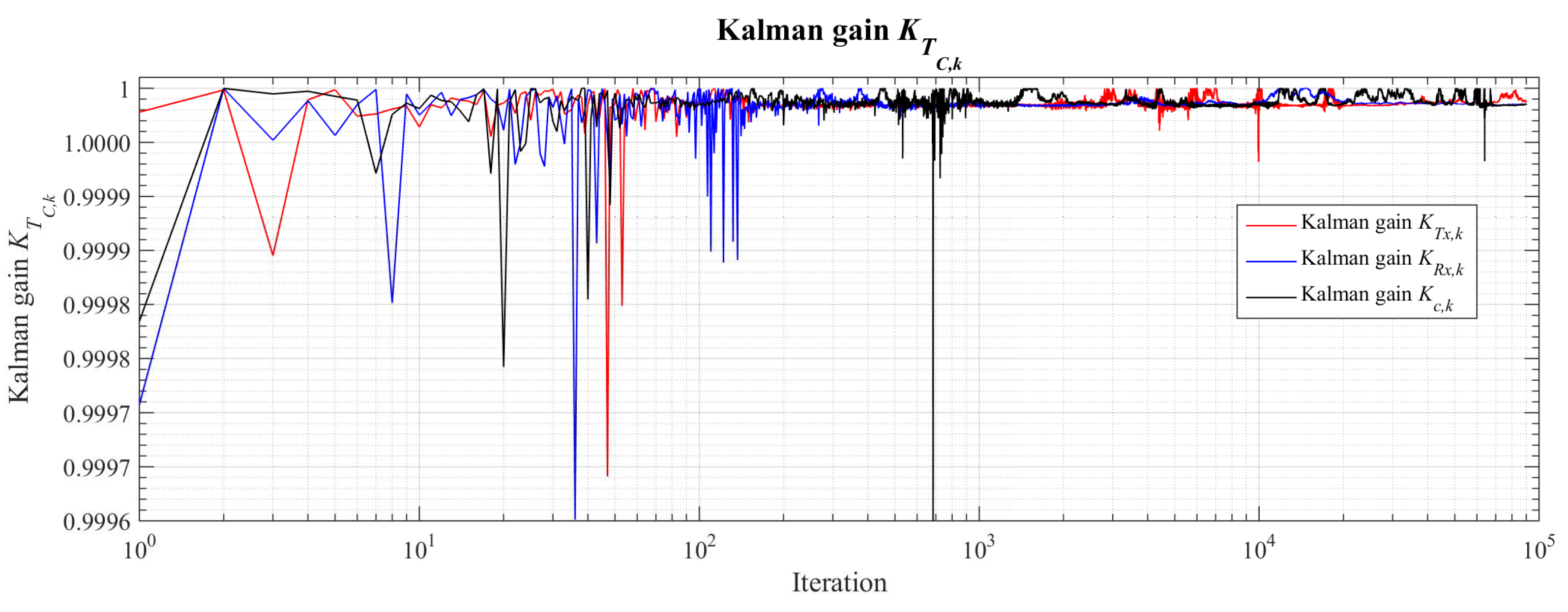
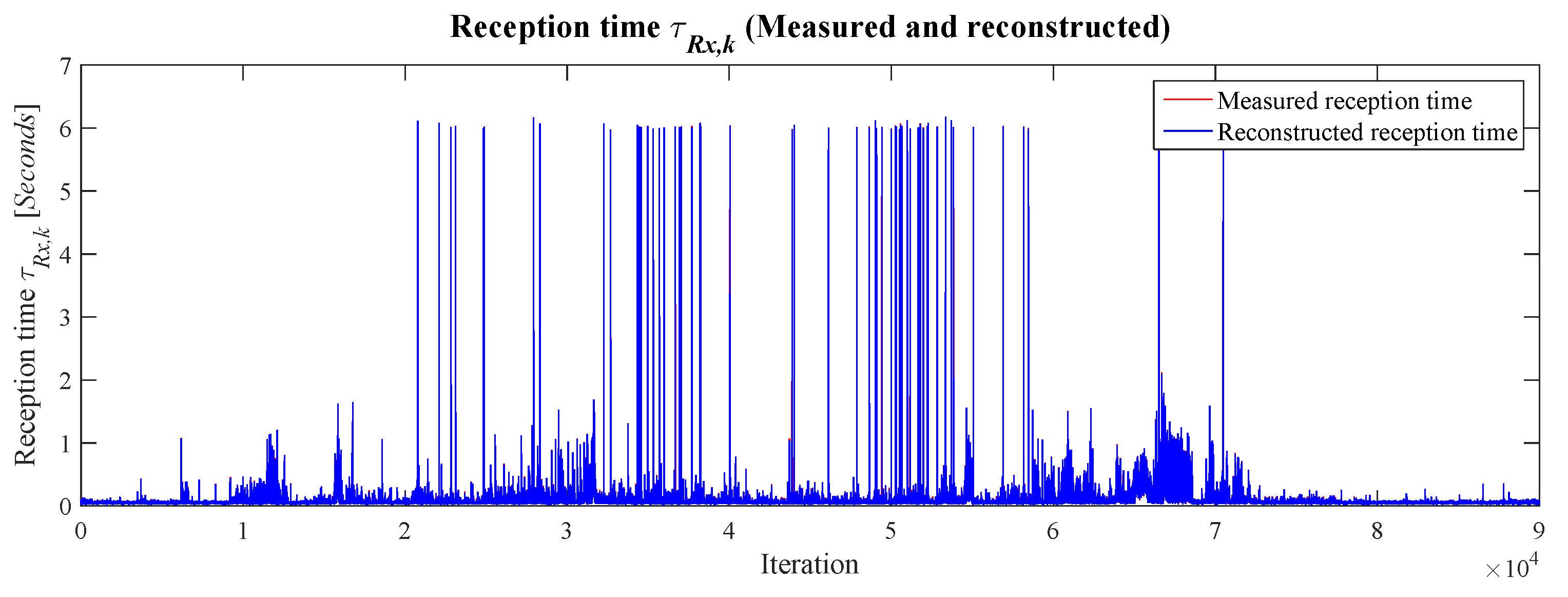
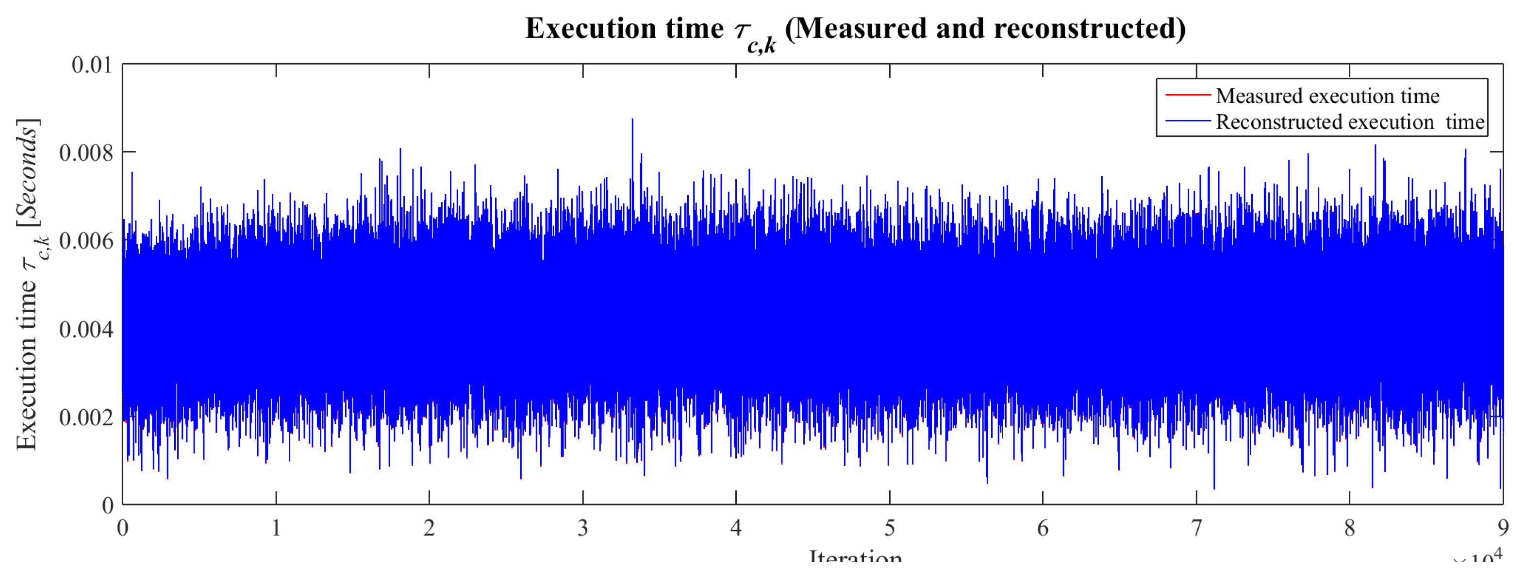
3.5. Reconstruction of Communication Times Using the Kalman Filter

Once linear independence of the noises associated with input system $Q_{T_{C,k}}$ and output system $R_{T_{C,k+1}}$ is ensured, it is possible to carry out the reconstruction of communication times. To this end, some additional implementation details of the Kalman filter are emphasized, so the description of the filter parameters settings is performed as follows:

$$A_k=\left[\begin{array}{ccc}13.686& 0& 0\\ 0& 12.786& 0\\ 0& 0& 15.86\end{array}\right]$$

(20)

$$B_k=\left[\begin{array}{ccc}0.96& 0& 0\\ 0& 0.99& 0\\ 0& 0& 0.94\end{array}\right]$$

(21)

$$C_k=\left[\begin{array}{ccc}1& 0& 0\\ 0& 1& 0\\ 0& 0& 1\end{array}\right]$$

(22)

$$U_k=\left[\begin{array}{c}0.004\\ 0.89\\ 0.15\end{array}\right]$$

(23)

Then, it is possible to use Equation (7) to calculate the Kalman’s gain $K_{T_{C,k}}$ (see Figure 12) that will allow the reconstruction of execution times ${\tau }_{c,k}$, reception times ${\tau }_{Rx,k}$, and transmission times ${\tau }_{Tx,k}$.

In Figure 13, the measured reception times ${\tau }_{Rx,k}$ and the reconstructed reception times ${\widehat{\tau }}_{Rx,k}$ can be observed. Here, it can be seen that the reconstruction of the reception times has the same behavior as the measured times.

Figure 14 presents the comparison between the measured execution times ${\tau }_{c,k}$ and the reconstructed execution times ${\widehat{\tau }}_{c,k}$.

Figure 15 presents the measured transmission times ${\tau }_{Tx,k}$ and the reconstructed transmission times ${\widehat{\tau }}_{Tx,k}$. Based on the comparison of the behavior of the measured and reconstructed times, it can be concluded that there is convergence in almost all points, so there is no difference between them.

In this case, as well as with ${\widehat{\tau }}_{Rx,k}$ and ${\widehat{\tau }}_{c,k}$, the obtained results are very close to the measured times $T_{C,k}$ for all values of k. However, it is considered that this argument is not enough, which leads to the use of descriptive measures such as the first- and second-order moment of probability, and the mean squared error to validate this result [3,27,30].

The behavior of the first order moment of probability $E\left\{T_{C,k}\right\}$ of the real and reconstructed communication times can be seen in Figure 16.

It can be seen that at the beginning of communication attempts using the TCP/IP protocol, communication times $T_{C,k}$ have a convergence towards the real values of almost 100% in most points.

The behavior of the second-order moment of probability $E{\left\{T_{C,k}\right\}}^2$ of the real and reconstructed communication times can be seen in Figure 17.

It can be seen that at the beginning of communication attempts using the TCP/IP protocol, the second-order moment of probability of reconstructed communication times ${\widehat{T}}_{C,k}$ has a certain divergence with respect to the real values, but once the system evolves, convergence towards real values is very close to 100% in almost all points.

For the probability density function, the frequency of appearance of the information of the transport times was measured through its histogram. A histogram is used to identify patterns in a data set when it is necessary to group the observations into a relatively small number of non-overlapping classes or bins, such that there is no imprecision in the class that a particular observation belongs. This grouping of observations for the information transport times is graphically observed in Figure 18, Figure 19 and Figure 20.

The mean squared error between real communication times $T_{C,k}$ and reconstructed communication times ${\widehat{T}}_{C,k}$ can be determined by describing the convergence of the filter by using (24) and (25) until the minimum magnitude of $H_{TC,k}$ is reached.

$$e_{T_{C,k}}={\widehat{T}}_{C,k}-T_{C,k}$$

(24)

$$H_{T_{C,k}}={\left[\frac{1}{k}((k-1)H_{T_{C,k-1}}+e_{T_{C,k}}^2)\right]}^{\frac{1}{2}}$$

(25)

Then, in Figure 21 and according to Equation (25), the Kalman filter has a convergence at almost all points since the mean squared error $H_{TC,k}$ converges to very small values (See

Table 4. Mean squared error $H_{T_{C,k}}$.

${\mathit{H}}_{\mathit{Tx},\mathit{k}}$	${\mathit{H}}_{\mathit{Rx},\mathit{k}}$	${\mathit{H}}_{\mathit{c},\mathit{k}}$
195.2 × 10−6	53.91 × 10−6	16.86 × 10−6

) for communication times $T_{C,k}$, which allows us to describe the quality of reconstruction, because the smaller the values of $H_{T_{C,k}}$, the better the reconstruction achieved.

4. Discussion

In a real-time system, execution times or computing times ${\tau }_{c,k}$ vary due to a variety of factors, such as deep pipeline, branch prediction [9], cache sizes [10], the worst-case execution path due to mutual exclusion [11], and other interactions, that cause non-deterministic behavior of execution times and are asynchronous in the dynamics system [12,13].

In telecontrol systems, reception times ${\tau }_{Rx,k}$ and transmission times ${\tau }_{Tx,k}$, the variation with respect to time is due to the fact that its duration depends on the increase in technological infrastructure, seasonal or hourly factors, cyclic factors, irregular factors [22], and communications protocols used for the exchange of information [23]. The reception time ${\tau }_{Rx,k}\in {\Re }^{+}$ is a period of time in which information is sent from Client A to the telecontrol server in an interval $k\in Z^{+}$. While the transmission time ${\tau }_{Tx,k}\in {\Re }^{+}$ is the time it takes to send information from the server to remote Client A in an interval $k\in Z^{+}$. In this sense, telecontrol time in real-time $T_{Tc,k}\in {\Re }^{+}$ is the algebraic sum of execution time ${\tau }_{c,k}$, reception time ${\tau }_{Rx,k}$, and transmission time ${\tau }_{Tx,k}$ in an interval $k\in Z^{+}$.

According to the previous paragraphs, to obtain telecontrol times measurement, in this paper the software architecture uses a modular multi-client–server communication scheme as workbench. The server implementation was performed on a dual processor computer with a speed of 1.6 GigaHertz, 4 Gigabytes of RAM, and the QNX 6.5 Neutrino real-time operating system [33]. Basically, the server executed three real-time tasks. The first task realized the communication via Internet to Client A and B using TCP/IP protocol through the use of function $socket\left(\right)$ from library $sys/socket.h$ [33]. The second server task was responsible for the simulation of an unstable first-order system. The third task of the server was programmed to obtain the measurement of communication times involved in the telecontrol process from server to Client A, within which execution times ${\tau }_{c,k}$, reception times ${\tau }_{Rx,k}$, and transmission times ${\tau }_{Tx,k}$ can be considered.

Once linear independence of the noises associated with input system $Q_{T_{C,k}}$ and output system $R_{T_{C,k+1}}$ was ensured, the Kalman filter was used as one part of a reconstructor of communication times $T_{C,k}$ of a telecontrol system. For this reason, it was necessary to analyze the covariance of input noise $Q_{T_{C,k}}$ and the covariance of output noise $R_{T_{C,k+1}}$ in execution times ${\tau }_{c,k}$, reception times ${\tau }_{Rx,k}$, and transmission times ${\tau }_{Tx,k}$. Then it is possible to use Equation (7) to calculate the Kalman’s gain $K_{T_{C,k}}$, which will allow the reconstruction of execution times ${\tau }_{c,k}$, reception times ${\tau }_{Rx,k}$, and transmission times ${\tau }_{Tx,k}$.

In this paper, the validation of the results is corroborated based on three descriptive measures: probability moments, probability distribution, and mean square error. All these measures are global indicators of the performance of the communication time reconstruction process. Regarding the probability moments, it is worth mentioning that they were analyzed for both measured and reconstructed communication times, and when comparing them in both scenarios, as shown in Figure 16 and Figure 17, they converge to similar values, validating that the reconstruction was successfully achieved. Regarding the probability distributions shown in Figure 19 and Figure 20, these denote the frequency of occurrence of transmission and reception times through their histograms, where the histogram is used to identify patterns in a data set when it is necessary to group the observations in a relatively small number of non-overlapping classes so that there is no imprecision in the class to which a given observation belongs. In this context, when comparing these histograms, it can be seen that the probability of occurrence of the reconstructed transmission and reception times is very similar to that of the measured ones. Therefore, in a probability sense, this argument also validates that the reconstruction process was performed adequately. Finally, the mean square errors defined by Equations (18) and (19) shown in Figure 21 have an asymptotic convergence to zero, which allows us to conclude that this performance indicator confirms the quality of the reconstruction obtained by means of the two approaches mentioned above.

It can be seen that at the beginning of communication attempts using the TCP/IP protocol, the second order moment of probability of reconstructed communication times ${\widehat{T}}_{C,k}$ has a certain divergence with respect to the real values, but once the system evolves, it converges towards real values very close to 100% in almost all points.

5. Conclusions

For the reconstruction of communication times dynamic $T_{C,k}$ using the Kalman filter, we present the following results.

(1) We observed in bibliographic references presented that the quantification of communication times $T_{C,k}$ of information over the Internet has a strong dependence on applications developed to work on the Internet, as well as factors that increase communication time, favoring the appearance of delay response times. Moreover, its modeling is based on structural models that depend on the type of information that is handled (voice, video, or data), which takes into account the size of information and amount of sent information. However, these models do not investigate the dynamics of communication times; thus, as a contribution to this work, we propose a modeling and reconstruction of the dynamic variation of communication times $T_{C,k}$ in telecontrol real-time systems using a model based on the Kalman filter.

(2) The Kalman filter has the ability to dynamically interpret the variables of a system and their respective variations.This interpretation gives a natural response according to the requirements of a process, ensuring proper operation.

(3) The reconstruction from the used method was quite good, since the communication times ${\widehat{T}}_{C,k}$ reconstructed in the telecontrol real-time system are very close to the real communication times $T_{C,k}$ for all values of k. We obtained an approximation very close to 100% in the first- and second-order moments of probability, achieving a mean squared error close to zero.

For future work, we expect to experiment with SIMO, MISO, and MIMO systems. This requires the scheduling of multiple processes that can be executed concurrently or in parallel to obtain a real-time simulation to meet the time constraints (deadline) associated with the dynamics of the system to be controlled.

One of the main focuses of the present research was the reconstruction of the communication times implicit in an experimental telecontrol scheme. For this purpose, the Kalman filter was used as an example of the application of adaptive digital filtering techniques. It is worth mentioning that for the development of the work and to deepen its study, some tasks were programmed in real-time, using for this purpose a real-time operating system. The reconstruction reported in the manuscript was validated according to the following criteria:

• Mean square error analysis.
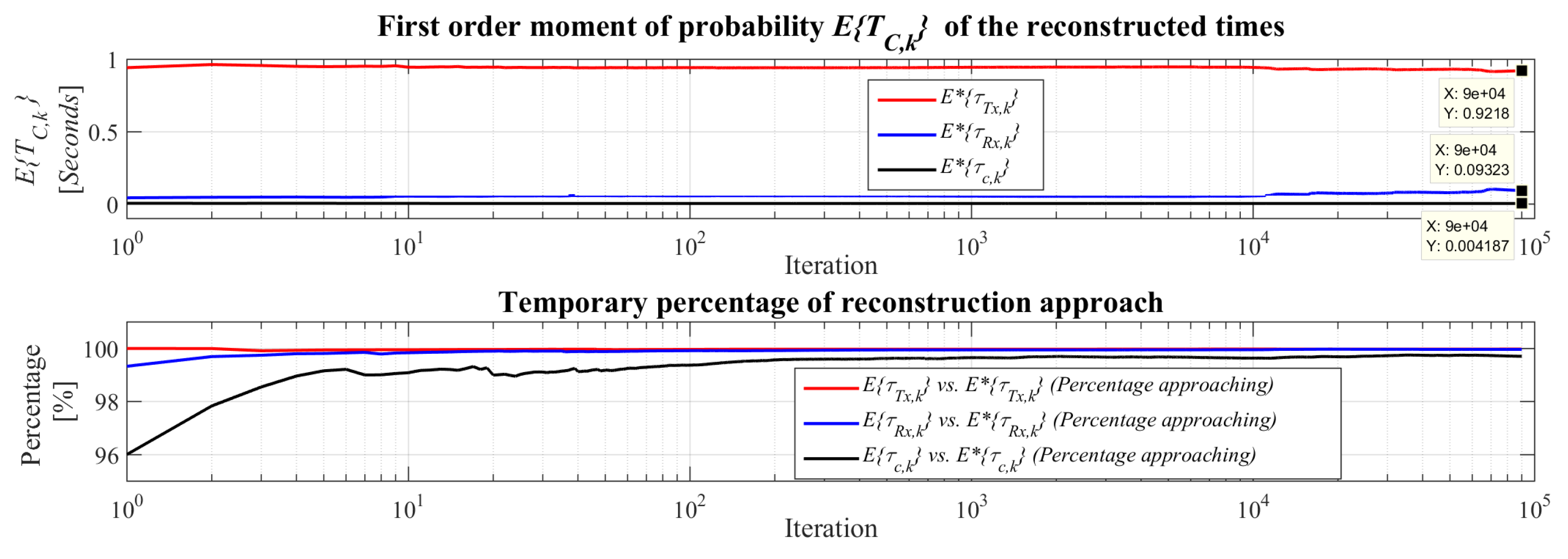
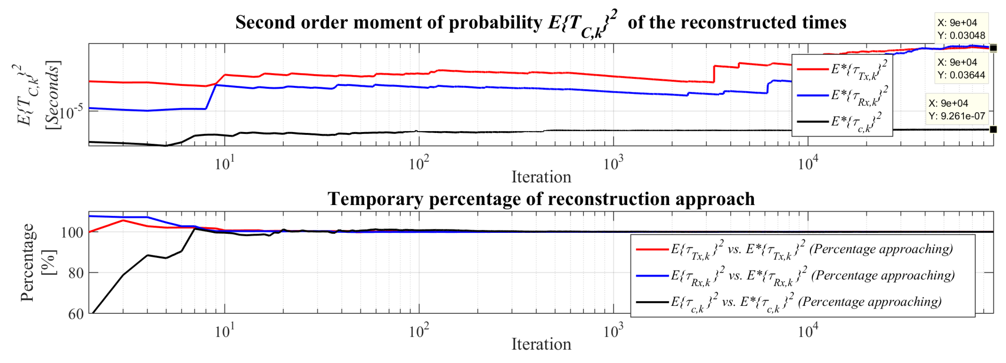
• Probability moment analysis
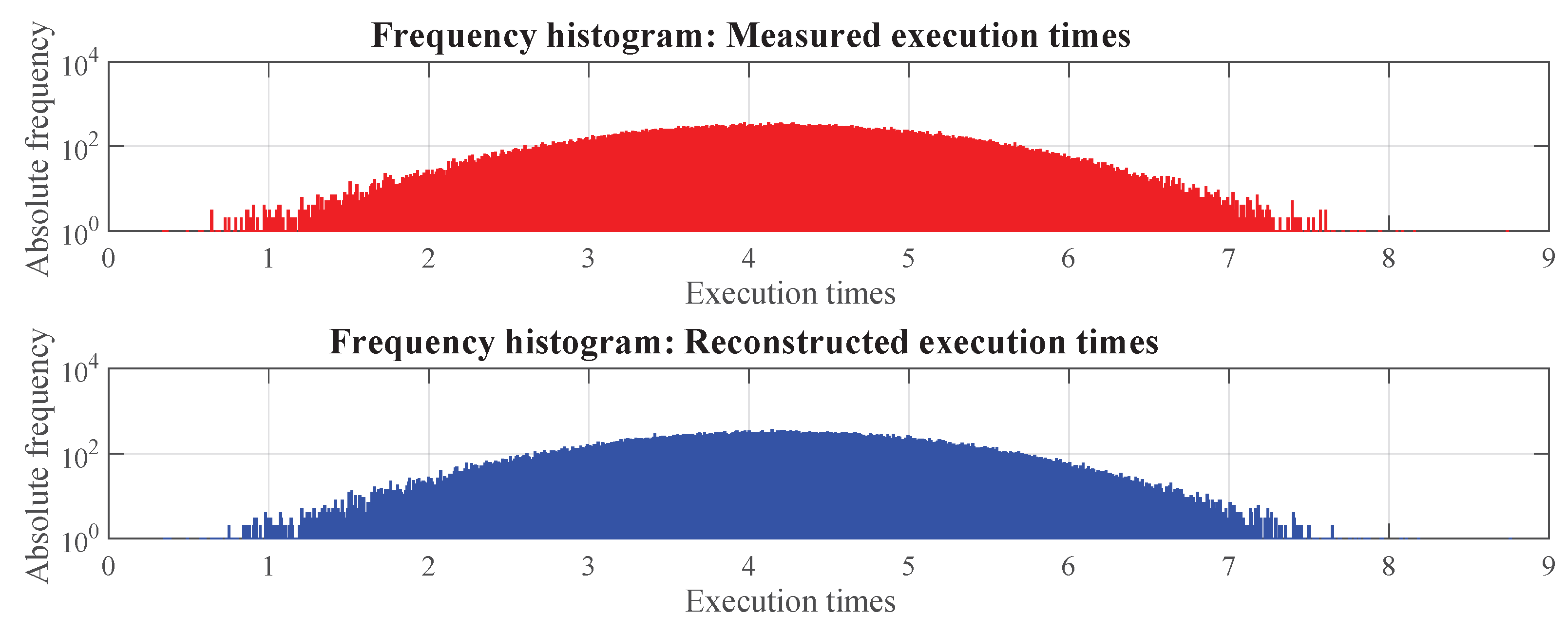
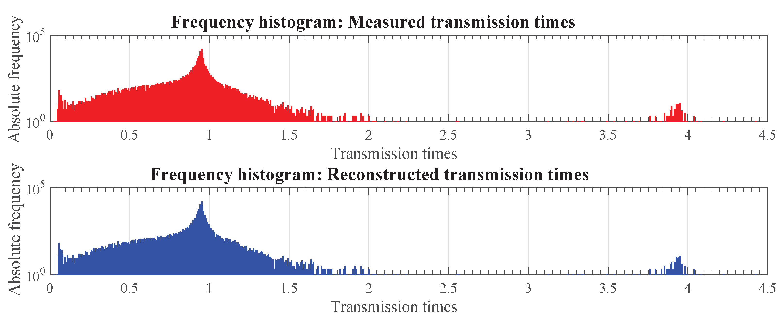
• Probability distribution analysis

Since the context of the manuscript concerns the aforementioned topic, it is proposed that the study of computational time complexity be carried out as future work. However, it should be noted that this approach could be developed according to the previous work developed by the authors of this paper cited in this manuscript [15].

References

1. Chessen, R.; Goldberg, N.; Piñeres, D. Comments of NCTA—The Internet & Television Association; NCTA—The Internet & Television Association: Washington, DC, USA, 2021; pp. 1–2. [Google Scholar]
2. Valdez Martínez, J.S. Medición, Caracterización y Reconstrucción de los Tiempos de Ejecución y Transporte para Sistemas de Telecontrol en Tiempo Real. Ph.D. Thesis, Instituto Politécnico Nacional, Mexico City, Mexico, 2015; pp. 1–210. [Google Scholar]
3. Valdez Martínez, J.S.; Guevara López, P. Measurement, Characterization and Reconstruction of Computing Time and Transporting Time for Real-Time Telecontrol Systems. Comput. Sist. 2019, 23, 531–546. [Google Scholar] [CrossRef]
4. Nyquist, H. Certain Topics in Telegraph Transmission Theory. Trans. Am. Inst. Electr. Eng. 1928, 47, 617–644. [Google Scholar] [CrossRef]
5. Kotel’nikov, V.A. On the transmission capacity of “ether” and wire in electrocomunications. Phys.-Uspekhi 2006, 49, 736. [Google Scholar] [CrossRef]
6. Padilla, J.J. Análisis del Comportamiento del tráfico en Internet durante la Pandemia del COVID-19: El caso de Colombia. Entre Cienc. Ing. 2020, 14, 26–33. [Google Scholar] [CrossRef]
7. Valdés, L.; Ariza, A.; Allende, S.M.; Triviño, A.; Joya, G. Search of the Shortest Path in a Communication Network with Fuzzy Cost Functions. Symmetry 2021, 13, 1534. [Google Scholar] [CrossRef]
8. Alzate, M.; Peña, N. Modelos de Tráfico en Análisis y Control de Redes de Comunicaciones. Rev. Ing. 2004, 9, 63–87. [Google Scholar]
9. Kumar, V. Deep Neural Network Approach to Estimate Early Worst-Case Execution Time. CoRR 2021, arXiv:abs/2108.02001. [Google Scholar]
10. Stappert, F.; Altenbernd, P. Complete Worst-Case Execution Time Analysis of Straight-line Hard Real Time Programs. J. Syst. Archit. Euromicro J. 2000, 46, 339–355. [Google Scholar] [CrossRef]
11. Bernat, G.; Colin, A.; Petters, S.M. PWCET: A tool for probabilistic Worst-Case Execution Time Analysis of Real-Time Systems; Technical Report YCS-2003-353; Department of Computer Science, University of York: York, UK, 2003; pp. 1–18. [Google Scholar]
12. Singh, A.; Nguyen, M.; Purawat, S.; Crawl, D.; Altintas, I. Modular Resource Centric Learning for Workflow Performance Prediction. arXiv 2017, arXiv:1711.05429. [Google Scholar]
13. Kshemkalyani, A.; Singhal, M. Chapter 15: Failure detectors. In Distributed Computing Principles, Algorithms, and Systems; Cambridge University Press: New York, NY, USA, 2011; pp. 567–597. [Google Scholar]
14. Hartmanis, J.; Stearns, R.E. On the computational complexity of algorithms. Trans. Am. Math. Soc. 1965, 117, 285–306. [Google Scholar] [CrossRef]
15. Delgado-Reyes, G.; Valdez-Martínez, J.S.; Hernández-Pérez, M.A.; Pérez-Daniel, K.R.; García-Ramírez, P.J. Quadrotor Real-Time Simulation: A Temporary Computational Complexity-Based Approach. Mathematics 2022, 10, 2032. [Google Scholar] [CrossRef]
16. Valdez Martínez, J.S.; Guevara Lopez, P.; Delgado Reyes, G. Execution Times Reconstruction in a LTI System Real-time Simulation. IEEE Lat. Am. Trans. 2014, 12, 277–284. [Google Scholar] [CrossRef]
17. Valdez Martínez, J.S.; Delgado Reyes, G.; Guevara Lopez, P.; Garcia Infante, J.C. Reconstruction of the execution times dynamics of real-time tasks by fuzzy digital filtering. Rev. Fac. Ing. Univ. Antioq. 2014, 70, 155–166. [Google Scholar]
18. Medel Juarez, J.J. Analysis of two estimation methods for stationary and invariant in time linear systems with disturbances correlated with the observable state of the type: One input one output. Comput. Sist. 2002, 5, 215–222. [Google Scholar]
19. Soderstrom, T.; Stoica, P. On some system identification techniques for adaptive filtering. IEEE Trans. Circuits Syst. 1988, 35, 457–461. [Google Scholar] [CrossRef]
20. Garcia Infante, J.C. Real-Time Fuzzy Digital Filtering. Comput. Sist. 2008, 11, 390–401. [Google Scholar]
21. Vázquez, B.; Garcia, I.; Sánchez, G.C. Description of adaptive fuzzy filtering using the DSP TMS320C6713. Proceedings of 2009 52nd IEEE International Midwest Symposium on Circuits and Systems, Cancun, Mexico, 2–5 August 2009; pp. 1086–1090. [Google Scholar]
22. Antonini, M.; De Luise, A.; Ruggieri, M.; Teotino, D. Satellite Data Collection and Forwarding systems. IEEE Aerosp. Electron. Syst. Mag. 2005, 20, 25–29. [Google Scholar] [CrossRef]
23. Karasawa, Y. On physical limit of wireless digital transmission from radio wave propagation perspective. Radio Sci. 2016, 51, 1600–1612. [Google Scholar] [CrossRef]
24. Casilari, E. Caracterización y Modelado de tráfico de Video VBR. Ph.D. Thesis, Universidad de Málaga, Málaga, Spain, 1998; pp. 1–406. [Google Scholar]
25. Luque, J. Modelado del Retardo de Transmisión en Bluetooth 2.0+EDR. Ph.D. Thesis, Universidad de Málaga, Málaga, Spain, 2010; pp. 1–370. [Google Scholar]
26. Rincon, D. Introducción a los modelos de tráfico para redes de banda ancha. Ramas Estud. IEEE 1998, 11, 41–48. [Google Scholar]
27. Valdez Martínez, J.S.; Villanueva Tavira, J.; Beltrán Escobar, M.A.; Contreras Calderon, E.; Alcalá Barojas, I.; López Vega, L.J. Analysis of the communication time of embedded systems applied to telecontrol systems. In Proceedings of the 2019 International Conference on Mechatronics, Electronics and Automotive Engineering (ICMEAE), Cuernavaca, Mexico, 26–29 November 2019; pp. 152–158. [Google Scholar]
28. Haykin, S. Adaptive Filter Theory, 2nd ed.; Prentice Hall: Hoboken, NJ, USA, 1991; pp. 210–215. [Google Scholar]
29. Nagurney, A. Mathematical Models of Transport and Networks. In Matematical Models in Economics, V II; EOLSS Publications: Abu Dhabi, United Arab Emirates, 2010; pp. 346–384. [Google Scholar]
30. Valdez Martínez, J.S.; Delgado Reyes, G.; Guevara Lopez, P.; Cano Rosas, J.L. Transmission Times Reconstruction in a Telecontrolled Real-Time System. IEEE Lat. Am. Trans. 2019, 17, 349–357. [Google Scholar] [CrossRef]
31. Gustafsson, F. Adaptive Filtering and Change Detection, 2nd ed.; John Wiley and Sons, Ltd.: Hoboken, NJ, USA, 2000; pp. 263–327. [Google Scholar]
32. Delgado Reyes, G.; Guevara Lopez, P.; De la Barrera, A.; Hernández, C.A. Uso del Filtro de Kalman para la Reconstruccion Adaptativa del Vector de Tiempos de Ejecución en la Simulación en Tiempo Real de un Motor de C. C. In Proceedings of the XI Congreso Internacional Sobre Innovación y Desarrollo Tecnológico CIINDET 2014, Cuernavaca, México, 2–4 April 2014. [Google Scholar]
33. Real-Time Operating System QNX Web Page. Available online: http://www.qnx.com/developers/docs/ (accessed on 22 November 2021).
34. Institute of Electrical and Electronics Engineers. Portable Operating System Interface (POSIX)-Part 1: System Application Program Interface (API) [C Language]; Institute of Electrical and Electronics Engineers: Manhattan, NY, USA, 1995. [Google Scholar]
35. González-Baldovinos, D.L.; Guevara-López, P.; Cano-Rosas, J.L.; Valdez-Martínez, J.S.; López-Chau, A. Response Times Reconstructor Based on Mathematical Expectation Quotient for a High Priority Task over RT-Linux. Mathematics 2022, 10, 134. [Google Scholar] [CrossRef]
36. National Instruments: Labview 2016 Web Page. Available online: https://www.ni.com/es-mx/shop/labview.html (accessed on 22 November 2021).
37. MATLAB Web Page. Available online: http://www.matlab.com/ (accessed on 22 November 2021).
Figure 1. Proposed telecontrol scheme.
Mathematics 10 03885 g001
Figure 2. Block diagram of Kalman filtering for communication times reconstruction.
Mathematics 10 03885 g002
Figure 3. User interface flow diagram developed for the telecontrol server.
Mathematics 10 03885 g003
Figure 4. User interface flow diagram developed for Client A in the telecontrol system.
Mathematics 10 03885 g004
Figure 5. Block diagram of the control system.
Mathematics 10 03885 g005
Figure 6. Client B front panel.
Mathematics 10 03885 g006
Figure 7. G Code diagram developed for Client B.
Mathematics 10 03885 g007
Figure 8. Reception times τ R x , k and transmission times τ T x , k using the TCP protocol measured by the server.
Mathematics 10 03885 g008
Figure 9. Execution times τ c , k measured in Client A.
Mathematics 10 03885 g009
Figure 10. Temporary behavior of covariances Q T C , k and R T C , k + 1 (using log scale on x- and y-axis).
Mathematics 10 03885 g010
Figure 11. Temporary behavior of the covariance of the identification error P T C , k + 1 (using log scale on x- and y-axis).
Mathematics 10 03885 g011
Figure 12. Temporary Kalman gain K T C , k for the reconstruction of communication times T C , k (using log scale on x-axis).
Mathematics 10 03885 g012
Figure 13. Comparison of reception times τ R x , k measured and reconstructed.
Mathematics 10 03885 g013
Figure 14. Comparison of execution times τ c , k measured and reconstructed.
Mathematics 10 03885 g014
Figure 15. Comparison of transmission times τ R x , k measured and reconstructed.
Mathematics 10 03885 g015
Figure 16. First order moment of probability E { T C , k } of communication times (using log scale on x-axis).
Mathematics 10 03885 g016
Figure 17. Second-order moment of probability E { T C , k } 2 of communication times (using log scale on x-axis).
Mathematics 10 03885 g017
Figure 18. Measured and reconstructed execution times frequency histogram (using log scale on x- and y-axis).
Mathematics 10 03885 g018
Figure 19. Measured and reconstructed transmission times frequency histogram (using log scale on x- and y-axis).
Mathematics 10 03885 g019
Figure 20. Measured and reconstructed reception times frequency histogram (using log scale on x- and y-axis).
Mathematics 10 03885 g020
Figure 21. Mean squared error H T C , k (using log scale on x- and y-axis).
Mathematics 10 03885 g021