Computational Analysis of Fractional Diffusion Equations Occurring in Oil Pollution

Abstract

The fractional model of diffusion equations is very important in the study of oil pollution in the water. The key objective of this article is to analyze a fractional modification of diffusion equations occurring in oil pollution associated with the Katugampola derivative in the Caputo sense. An effective and reliable computational method q-homotopy analysis generalized transform method is suggested to obtain the solutions of fractional order diffusion equations. The results of this research are demonstrated in graphical and tabular descriptions. This study shows that the applied computational technique is very effective, accurate, and beneficial for managing such kind of fractional order nonlinear models occurring in oil pollution.

1. Introduction

Fractional derivatives are a particular aid of applied mathematics that are related to non-integer order derivatives and integrals. Recently, pioneering work in this notable branch has been carried in several scientific, engineering, and in different another crucial fields. In fact, the new characteristics of this notable branch are affected by distinct useful applications, for example in fluid flow problems, electrochemistry, plasma physics, mathematical biology, turbulence, image processing, astrophysics, controlled thermonuclear fusion, control theory, and many more. In view of the aforementioned facts, it is noteworthy that the derivatives and integral of fractional orders have appeared as a pivotal novel mathematical key for solving the several issues in science and engineering fields. The significant advantage of fractional calculus is about to model the physical problems having whole memory effect. Miller and Ross [1] wrote a book about the introduction to fractional calculus and differential equations of fractional order. Podlubny [2] provided detailed information about arbitrary order differential equations. Caputo [3] reported about fundamental properties of fractional calculus. Singh [4] studied a blood alcohol model of fractional order. Caputo and Fabrizio [5] explained new features of fractional derivative. Caputo and Fabrizio [6] discussed about singular kernels associated to fractional derivatives. Singh et al. [7] investigated a computational scheme for local fractional transport equation. Singh et al. [8] examined a reliable computational technique for local fractional Poisson equation arising in fractal media. Yang [9] analyzed a novel integral transform operator to solve heat diffusion equation. Losada and Nieto [10] discussed about the characteristic of novel non-integer order derivative without singular kernel. Atangana and Baleanu [11] investigated novel arbitrary order derivative having nonlocal and non-singular kernel. Kumar et al. [12] studied an advanced computational scheme with convergence analysis for Lienard’s equation of arbitrary order.

Nonlinear partial differential equations (NPDE) play a very significant role in several fields, for example ocean engineering, fluid mechanics, astrophysics, plasma physics, solid-state physics, optical fiber, ocean ecology, metrology, and wave motion. Oil pollution occurs through the freeing of a fluid oil hydrocarbon within ocean surroundings due to human activities, for example freeing of petroleum without refining from drilling rigs, tankers, and offshore platforms, in addition to piping that may produce critical destruction to the marine ecological environment. Hence, to protect the natural shoreline environmental structure, it is important to exactly estimate the expand range of oil spills in relation to the advance stage correction against a calamity. By solving the proper equations governing the flow field additionally to the diffusion phenomenon, the zone of oil expanding can be expected numerically. The logical key option is likely a diffusion equations where detail regarding the quantity of oil, which outreaches the ocean outlet, can be considered as initial boundary conditions for modeling the oil diffusion in addition to adaptation in the waters.

To discuss oil pollution, we examine a general linear diffusion equation given as follows:

$$\frac{\partial \xi }{\partial \theta }=d\frac{{\partial }^2\xi }{\partial {\vartheta }^2}+a\xi ,$$

(1)

where $\xi$ represents the concentration, $d$ indicates diffusion coefficient, and $a$ is a real constant. The generalization of Equation (1) becomes the Allen–Cahn (AC) equation. The AC equation is a parabolic partial differential equation which represents crucial natural physical aspects. It has been broadly applied to analyze many physical problems, such as fluid mechanics, quantum mechanics, chemical kinematics, optical fibers, propagation of shallow-water waves, and in other important field of science and engineering. To examine phase transitions and interfacial dynamics in the material science branch, the AC equation is considered a fundamental model for study the diffuse interface system. The AC equation is also employed to analyze phase separation into binary alloys which can be represented as a reaction–diffusion equation in case of material sciences and as a convection–diffusion equation in the case of fluid dynamics. Hariharan [13] discussed a reliable Legendre wavelet associate approximation technique for Newell–Whitehead with AC equations. Allen and Cahn [14] studied a microscopic concept for antiphase boundary motion in addition to its usefulness to antiphase domain coarsening. Shah et al. [15] examined a numerical algorithm to solve AC equation. Chen et al. [16] investigated an adaptive finite element technique for AC equation. Ahmad [17] studied about solutions of diffusion equations occurring in oil pollution. Bulut [18] discussed about few new exponential functions to the AC equation. Manafian [19] investigated about an optimal Galerkin-homotopy asymptotic technique employed for solving nonlinear second order bvps. Shahriari and Manafian [20] examined a reliable technique to solve the dirac differential operator in fractional sense. Dehghan et al. [21] explained homotopy analysis algorithm to solve nonlinear partial differential equations of fractional order.

Thus, the diffusion equation which is expressed by Equation (1) related with fractional order derivative would be an advancement to the diffusion equation. Since non-integer order derivatives are very crucial in the analysis of mathematical modeling of physical problems, in this article, we study the fractional order modification of diffusion equation which is represented by Equation (1). The diffusion equation of non-integer order is attained from classical order diffusion equation by changing the first order time derivative by the Katugampola arbitrary derivative in the Caputo sense [22]. The diffusion Equation (1) associated to the Katugampola derivative in the Caputo type is expressed as follows:

$${}_a{}^{KC}D{}_{\theta }^{\mu ,\eta }\xi =d\frac{{\partial }^2\xi }{\partial {\vartheta }^2}+a\xi ,$$

(2)

There are many numerical as well as analytical techniques to investigate aspects of such types of models. Liao [23,24] suggested an analytic scheme familiar as homotopy analysis method (HAM) to control nonlinear physical problems. El-Tawil and Huseen [25,26] have analyzed a modification of HAM familiar as q-homotopy analysis method (q-HAM) to represent behavior of non-linear real world problems. Since traditional analytic methods require additional computer memory as well as extra computing time, for controlling such kinds of limitations, analytical techniques require to be mixed with classical integral transforms to consider behavior of nonlinear mathematical models occurring in scientific and technological fields [27,28,29,30].

The key objective of this paper is to investigate a new numerical method that is q-homotopy analysis generalized transform method i.e., q-HAGTM for solving nonlinear fractional order diffusion equation. It is a strong amalgamation of q-HAM, generalized Laplace transform (GLT) in addition to homotopy polynomials. The supremacy of the suggested method is expressed by merging two powerful computing schemes to analyze nonlinear fractional order differential equations. Moreover, q-HAGTM carry an asymptotic parameter, say, n, which ensures convergence of series solution of physical models. The proposed method is a new study for fractional diffusion equation appearing in oil pollution associated with the Caputo–Katugampola fractional derivative. As per our best knowledge, this study has not been discussed in the literature.

In this paper, we study fractional diffusion equation occurring in oil pollution by applying q-HAGTM. This paper is organized as follows: Section 2 demonstrates about generalized Laplace transform and fractional derivatives. Section 3 presents the details about q-HAGTM. Section 4 imparts the numerical results and new aspects of fractional diffusion equation in three separate cases. Lastly, Section 6 elaborates the conclusion of the paper.

2. Mathematical Preliminaries

Important definitions and fractional operators [2,22,31,32,33,34,35] which are utilized in this manuscript are expressed in the following manner

Definition 1.

The Caputo derivative [2] of order $0\le \mu <1$ of the function $\xi (\theta )$ is given as

$${}_a{}^{C}D{}_{\theta }^{\mu }\xi (\theta )=\frac{1}{\mathsf{\Gamma }(1-\mu )}{\displaystyle \underset{a}{\overset{t}{\int }}{(\theta -v)}^{-\mu }}{\xi }^{\prime }(v)dv.$$

(3)

Definition 2.

The Caputo–Hadamard derivative [31] of order $0\le \mu <1$ of the function $\xi (\theta )$ is given as

$${}_a{}^{CH}D{}_t^{\mu }\xi (\theta )=\frac{1}{\mathsf{\Gamma }(1-\mu )}{\displaystyle \underset{a}{\overset{t}{\int }}{\left(\log \frac{\theta }{v}\right)}^{-\mu }\alpha }\frac{\xi (v)}{v}dv,$$

(4)

where $\alpha$ is differential operator and is defined by $\alpha =\theta \frac{d}{d\theta }.$

Definition 3.

The Katugampola derivative [22] in the Caputo type of order $0\le \mu <1$ of the function $\xi (\theta )$ is given as follows

$${}_a{}^{KC}D{}_{\theta }^{\mu ,\eta }\xi (\theta )=\frac{1}{\mathsf{\Gamma }(1-\mu )}{\displaystyle \underset{a}{\overset{\theta }{\int }}{\left(\frac{{\theta }^{\eta }-v^{\eta }}{\eta }\right)}^{-\mu }\beta }\frac{\xi (v)}{v^{1-\eta }}dv,$$

(5)

where$\beta$ is differential operator and is defined by $\beta ={\theta }^{1-\eta }\frac{d}{d\theta }.$

If we set $\eta =1,$ then the derivative given by Equation (5) reduces in the Caputo derivative with order $\mu .$ If $\eta$ tens to 0, then the derivative defined by Equation (5) reduces to the Caputo–Hadamard non-integer order derivative with order $\mu$.

Definition 4.

Suppose that $\xi ,\psi :[a,\infty )\to R$ be a real valued function in such manner that $\psi (\theta )$is continuous and ${\psi }^{\prime }(\theta )>0$ on $[a,\infty )$. If the GLT [32] of $\psi (\theta )$ exists, then

$$L_{\psi }\left\{\xi \left(\theta \right)\right\}\left(s\right)=\underset{a}{\overset{\infty }{{\displaystyle \int }}}{e}^{-s\left(\psi \left(\theta \right)-\psi \left(a\right)\right)}\xi \left(\theta \right){\psi }^{\prime }\left(\theta \right)d\theta ,$$

(6)

where $s$ denotes the GLT operator.

If we set$\psi (\theta )=\theta$and$a=0$in Equation (6), then GLT reduces in standard LT but if we set$\psi (\theta )=\frac{{\theta }^{\eta }}{\eta }$and$a=0$in this case the GLT converts in to the$\eta -$LT [33].

In this paper, we consider the GLT with $\psi (\theta )=\frac{{\theta }^{\eta }}{\eta }$ and $a=0$ by $\frac{{\theta }^{\eta }}{\eta }-$LT. The $\frac{{\theta }^{\eta }}{\eta }-$LT is defined by

$$L_{\frac{{\theta }^{\eta }}{\eta }}\left\{\xi (\theta )\right\}(s)={\displaystyle \underset{a}{\overset{\infty }{\int }}{e}^{-s\frac{{\theta }^{\eta }}{\eta }}}\xi (\theta )\frac{d\theta }{{\theta }^{1-\eta }}.$$

(7)

The $\frac{{\theta }^{\eta }}{\eta }-$LT of the Katugampola derivative in the Caputo sense [30,33] is given as follows

$$L_{\frac{{\theta }^{\eta }}{\eta }}\left\{\left({}^{KC}D{}_{\theta }^{\mu ,\eta }\xi \right)(\theta )\right\}(s)=s^{\mu }{L}_{\frac{{\theta }^{\eta }}{\eta }}\left\{f(\theta )\right\}(s)-s^{\mu -1}f(0).$$

(8)

3. Fundamental Plan of q-Homotopy Analysis Generalized Transform Method (q-HAGTM)

To discuss the principal scheme of proposed method, we study an NPDE associated to the Katugampola derivative as follows

$${}^{KC}D{}_{\theta }^{\mu ,\eta }\xi (\vartheta ,\theta )+M\xi (\vartheta ,\theta )+N\xi (\vartheta ,\theta )=f(\vartheta ,\theta ),n-1<\mu \le n,$$

(9)

where $D_{\theta }^{\mu ,\eta }\xi$ denotes the fractional derivative in the Caputo–Katugampola sense, $M$ and $N$ represent the general differential operators; additionally, $f(\vartheta ,\theta )$ denotes the source term.

First of all, we employ GLT on Equation (9), where we have

$$L_{\frac{{\theta }^{\eta }}{\eta }}[{}^{KC}D{}_{\theta }^{\mu ,\eta }\xi (\vartheta ,\theta )]+L_{\frac{{\theta }^{\eta }}{\eta }}[M\xi (\vartheta ,\theta )]+L_{\frac{{\theta }^{\eta }}{\eta }}[N\xi (\vartheta ,\theta )]=L_{\frac{{\theta }^{\eta }}{\eta }}[f(\vartheta ,\theta )].$$

(10)

Next, by utilizing differentiation formula of GLT, we obtain

$$s^{\mu }{L}_{\frac{{\theta }^{\eta }}{\eta }}[\xi (\vartheta ,\theta )]-s^{\mu -1}\xi (\vartheta ,0)+L_{\frac{{\theta }^{\eta }}{\eta }}[M\xi (\vartheta ,\theta )]+L_{\frac{{\theta }^{\eta }}{\eta }}[N\xi (\vartheta ,\theta )]=L_{\frac{{\theta }^{\eta }}{\eta }}[f(\vartheta ,\theta )].$$

(11)

Dividing both the sides of Equation (11) by and simplifying, we obtain

$$L_{\frac{{\theta }^{\eta }}{\eta }}[\xi (\vartheta ,\theta )]-\frac{1}{s}\xi (\vartheta ,0)+\frac{1}{s^{\mu }}\left[L_{\frac{{\theta }^{\eta }}{\eta }}[M\xi (\vartheta ,\theta )]+L_{\frac{{\theta }^{\eta }}{\eta }}[N\xi (\vartheta ,\theta )]-L_{\frac{{\theta }^{\eta }}{\eta }}[\xi (\vartheta ,\theta )]\right]=0.$$

(12)

Now we represent an operator given as follows

$$\begin{array}{ll}N[\phi (\vartheta ,\theta ;q)]=& L_{\frac{{\theta }^{\eta }}{\eta }}[\phi (\vartheta ,\theta ;q)]-\frac{1}{s}\phi (\vartheta ,\theta ;q)(0^{+})+\\ & \frac{1}{s^{\mu }}\left[L_{\frac{{\theta }^{\eta }}{\eta }}[M\phi (\vartheta ,\theta ;q)]+L_{\frac{{\theta }^{\eta }}{\eta }}[N\phi (\vartheta ,\theta ;q))]-L_{\frac{{\theta }^{\eta }}{\eta }}[f(\vartheta ,\theta )]\right]=0.\end{array}$$

(13)

Here, $q\in [0,1/n]$ and $\phi (\vartheta ,\theta ;q)$ represents a real function. Next, we set a homotopy in the subsequent approach

$$(1-nq)L_{\frac{{\theta }^{\eta }}{\eta }}[\phi (\vartheta ,\theta ;q)-{\xi }_0(\vartheta ,\theta )]=ħqH(\vartheta ,\theta )N[\xi (\vartheta ,\theta )],$$

(14)

where $n\ge 1,$ $H(\vartheta ,\theta )\ne 0$ denotes an auxiliary function, $ħ\ne 0$ indicates auxiliary parameter, ${\xi }_0(\vartheta ,\theta )$ represents an initial guess of $\xi (\vartheta ,\theta )$ and $\phi (\vartheta ,\theta ;q)$ denotes an unknown function. When we put $q=0$ and $q=\frac{1}{n},$ we have the following outcomes

$$\phi (\vartheta ,\theta ;0)={\xi }_0(\vartheta ,\theta ),\phi (\vartheta ,\theta ;\frac{1}{n})=\xi (\vartheta ,\theta ).$$

(15)

Thus, when $q$ tends 0 to $\frac{1}{n}$, $\phi (\vartheta ,\theta ;q)$ changes from ${\xi }_0(\vartheta ,\theta )$t to the solution $\xi (\vartheta ,\theta ).$ Expanding $\phi (\vartheta ,\theta ;q)$ in a series expression by utilizing Taylor’s theorem about parameter $q$, we obtain

$$\phi (\vartheta ,\theta ;q)={\displaystyle \sum _{l=0}^{\infty }{\xi }_l(\vartheta ,\theta )q^l}.$$

(16)

Here, the value of ${\xi }_l(\vartheta ,\theta )$ is given as follows

$${\xi }_l(\vartheta ,\theta )=\frac{1}{l!}\frac{{\partial }^l\phi (\vartheta ,\theta ;q)}{\partial q^l}|{}_{q=0}.$$

(17)

Now we select the value of ${\xi }_0(\vartheta ,\theta )$, the parameters $n,ħ$ and $H(\vartheta ,\theta )$, the parameters $n,ħ$ and in such a way that Equation (14) converges at $q=\frac{1}{n,}$, then we have

$$\xi (\vartheta ,\theta )={\displaystyle \sum _{l=0}^{\infty }{\xi }_l(\vartheta ,\theta )}{(\frac{1}{n})}^l.$$

(18)

The above is one of solution of the original nonlinear equation. The governing equation can be attained from Equation (14) by taking in consideration the solution given in (18).

Now we set the vectors as follows

$${\overline{\xi }}_l=\{{\xi }_0,{\xi }_1,\dots ,{\xi }_l\}.$$

(19)

We differentiate Equation (14) l-times about $q$ and then divide by $l!$ further taking $q=0,$ then deformation equation of $l$th-order is given as follows

$$L_{\frac{{\theta }^{\eta }}{\eta }}[{\xi }_l(\vartheta ,\xi )-{\kappa }_l{\xi }_{l-1}(\vartheta ,\xi )]=ħH(\vartheta ,\xi ){\mathsf{\Theta }}_l({\overline{\xi }}_{l-1}).$$

(20)

Next, by exerting the inverse Laplace operator, we obtain

$${\xi }_l(\vartheta ,\theta )={\kappa }_l{\xi }_{l-1}(\vartheta ,\theta )+ħL_{\frac{{\theta }^{\eta }}{\eta }}{}^{-1}[H(\vartheta ,\theta ){\mathsf{\Theta }}_l({\overline{\xi }}_{l-1})].$$

(21)

The value of ${\mathsf{\Theta }}_l({\overline{\xi }}_{l-1})$ is represented in the following way

$${\mathsf{\Theta }}_l({\overline{\xi }}_{l-1})=\frac{1}{(l-1)!}\frac{{\partial }^{l-1}N[\phi (\vartheta ,\theta ;q)]}{\partial q^{l-1}}|{}_{q=0},$$

(22)

where

$${\kappa }_l=\{\begin{array}{l}0,\hspace{1em}l\le 1,\\ n,\hspace{1em}l>1.\end{array}$$

(23)

When we set $n=1,$ then q-HAGTM solution converts in to HAGTM solution.

4. Numerical Solution of Fractional Diffusion Equations Occurring in Oil Pollution

Here, we discuss numerical outcomes of fractional order diffusion equation and AC equations occurring in oil pollution by applying the proposed q-HAGTM.

Example 1.

First, we study time-fractional diffusion equation as follows

$$\frac{\partial \xi (\vartheta ,\theta )}{\partial \theta }=\frac{{\partial }^2\xi (\vartheta ,\theta )}{\partial {\vartheta }^2}+\cos \vartheta ,$$

(24)

with the initial condition

$$\xi (\vartheta ,0)=0,\xi (0,\theta )=1-e^{-\theta },\xi (1,\theta )=-1+e^{-\theta }.$$

(25)

The exact solution of Equation (24) is given as follows

$$\xi (\vartheta ,\theta )=\cos \vartheta (1-e^{-\theta }).$$

(26)

Since the integer order mathematical model does not impart past memory of the model, for considering the whole memory of diffusion equation we replace the classical derivative of Equation (24) by the Caputo–Katugampola fractional order derivative, then we have

$${}^{KC}D{}_{\theta }^{\mu ,\eta }\xi (\vartheta ,\theta )=\frac{{\partial }^2\xi (\vartheta ,\theta )}{\partial {\vartheta }^2}+\cos \vartheta ,$$

(27)

with initial condition given by Equation (26).

Now by employing GLT both the sides of Equation (27), we obtain

$$L_{\frac{{\theta }^{\eta }}{\eta }}\left[{}^{KC}D{}_{\theta }^{\mu ,\eta }\xi (\vartheta ,\theta )\right]=L_{\frac{{\theta }^{\eta }}{\eta }}\left[\frac{{\partial }^2\xi (\vartheta ,\theta )}{\partial {\vartheta }^2}+\cos \vartheta \right],$$

(28)

Now utilizing Equation (8) and Equation (26), we have

$$L_{\frac{{\theta }^{\eta }}{\eta }}\left\{\xi (\vartheta ,\theta )\right\}-\frac{1}{s^{\mu }}{L}_{\frac{{\theta }^{\eta }}{\eta }}\left[\frac{{\partial }^2\xi (\vartheta ,\theta )}{\partial {\vartheta }^2}+\cos \vartheta \right]=0.$$

(29)

Next, we consider an operator represented in the following way

$$N\left[\phi \left(\vartheta ,\theta ;q\right)\right]=L_{\frac{{\theta }^{\eta }}{\eta }}\left[\phi \left(\vartheta ,\theta ;q\right)\right]-\frac{1}{s^{\mu }}{L}_{\frac{{\theta }^{\eta }}{\eta }}\left[\frac{{\partial }^2\xi \left(\vartheta ,\theta ;q\right)}{\partial {\vartheta }^2}+\cos \vartheta \right]=0,$$

(30)

and the value of ${\mathsf{\Theta }}_l({\overline{\xi }}_{l-1})$ is given as follows

$${\mathsf{\Theta }}_l({\overline{\xi }}_{l-1})=L_{\frac{{\theta }^{\eta }}{\eta }}[{\xi }_{l-1}]-\frac{1}{s^{\mu }}{L}_{\frac{{\theta }^{\eta }}{\eta }}\left[\frac{{\partial }^2{\xi }_{l-1}}{\partial {\vartheta }^2}+\cos \vartheta \right]$$

(31)

.

Next the deformation Equation of$l^{th}$order is given as follows

$$L_{\frac{{\theta }^{\eta }}{\eta }}[{\xi }_l(\vartheta ,\theta )-{\kappa }_l{\xi }_{l-1}(\vartheta ,\theta )]=ħ{\mathsf{\Theta }}_l(\overline{\xi }l-1).$$

(32)

Now by exerting inverse GLT on Equation (32), we have

$${\xi }_l(\vartheta ,\theta )={\kappa }_l{\xi }_{l-1}(\vartheta ,\theta )+ħL_{{}_{\frac{{\theta }^{\eta }}{\eta }}}^{-1}\left[{\mathsf{\Theta }}_l({\overline{\xi }}_{l-1})\right].$$

(33)

Further, by settg$l=1,2,3,\dots$we obtain

$${\xi }_1(\vartheta ,\theta )=-ħ\frac{\cos \vartheta }{\mathsf{\Gamma }(1+\mu )}{\left(\frac{{\theta }^{\eta }}{\eta }\right)}^{\mu },$$

(34)

$${\xi }_2(\vartheta ,\theta )=-ħ(n+ħ)\frac{\cos \vartheta }{\mathsf{\Gamma }(1+\mu )}{\left(\frac{{\theta }^{\eta }}{\eta }\right)}^{\mu }-ħ\frac{\cos \vartheta }{\mathsf{\Gamma }(1+\mu )}{\left(\frac{{\theta }^{\eta }}{\eta }\right)}^{\mu }-{ħ}^2\frac{\cos \vartheta }{\mathsf{\Gamma }(1+2\mu )}{\left(\frac{{\theta }^{\eta }}{\eta }\right)}^{2\mu },$$

(35)

and so on.

The series solution of Equation (24) is represented in the following approach

$$\xi (\vartheta ,\theta )={\xi }_0(\vartheta ,\theta )+\frac{1}{n}{\xi }_1(\vartheta ,\theta )+{\left(\frac{1}{n}\right)}^2{\xi }_2(\vartheta ,\theta )+\dots$$

(36)

Now substituting values of Equations (25), (34), and (35) in Equation (36), we have

$$\xi (\vartheta ,\theta )=-\frac{ħ}{n}\frac{\cos \vartheta }{\mathsf{\Gamma }(1+\mu )}{\left(\frac{{\theta }^{\eta }}{\eta }\right)}^{\mu }+{\left(\frac{1}{n}\right)}^2\left[\begin{array}{l}-ħ(n+ħ)\frac{\cos \vartheta }{\mathsf{\Gamma }(1+\mu )}{\left(\frac{{\theta }^{\eta }}{\eta }\right)}^{\mu }-ħ\frac{\cos \vartheta }{\mathsf{\Gamma }(1+\mu )}{\left(\frac{{\theta }^{\eta }}{\eta }\right)}^{\mu }\\ -{ħ}^2\frac{\cos \vartheta }{\mathsf{\Gamma }(1+2\mu )}{\left(\frac{{\theta }^{\eta }}{\eta }\right)}^{2\mu }\end{array}\right]+\dots$$

(37)

which a required solution of Equation (24) in series form.

Example 2.

Next, we study the time-fractional Allen–Cahn equation as follows

$$\frac{\partial \xi (\vartheta ,\theta )}{\partial \theta }=\frac{{\partial }^2\xi (\vartheta ,\theta )}{\partial {\vartheta }^2}+\vartheta (1-{\vartheta }^2),$$

(38)

with the initial condition

$$\xi (\vartheta ,\theta )=-0.5+0.5\tanh (0.3536\vartheta ).$$

(39)

The exact solution of Equation (38) is given as follows

$$\xi (\vartheta ,\theta )=-0.5+0.5\tanh (0.3536\vartheta -0.75\theta ).$$

(40)

Since integer order mathematical model does not impart past memory of the model, for considering the whole memory of AC equation, we replace the classical derivative of Equation (38) by the Caputo–Katugampola fractional order derivative, then we have

$${}^{KC}D{}_{\theta }^{\mu ,\eta }\xi (\vartheta ,\theta )=\frac{{\partial }^2\xi (\vartheta ,\theta )}{\partial {\vartheta }^2}+\vartheta (1-{\vartheta }^2),$$

(41)

with the initial condition given by Equation (39).

Now by employing GLT on both the sides of Equation (41), we have

$$L_{\frac{{\theta }^{\eta }}{\eta }}\left[{}^{KC}D{}_{\theta }^{\mu ,\eta }\xi (\vartheta ,\theta )\right]=L_{\frac{{\theta }^{\eta }}{\eta }}\left[\frac{{\partial }^2\xi (\vartheta ,\theta )}{\partial {\vartheta }^2}+\vartheta (1-{\vartheta }^2)\right].$$

(42)

Now utilizing Equation (8) and Equation (39), we have

$$L_{\frac{{\theta }^{\eta }}{\eta }}\left\{\xi (\vartheta ,\theta )\right\}-\frac{\xi (\vartheta ,0)}{s}-\frac{1}{s^{\mu }}{L}_{\frac{{\theta }^{\eta }}{\eta }}\left[\frac{{\partial }^2\xi (\vartheta ,\theta )}{\partial {\vartheta }^2}+\vartheta (1-{\vartheta }^2)\right]=0.$$

(43)

Next, we consider an operator described in the subsequent manner

$$\begin{array}{ll}N[\phi (\vartheta ,\theta ;q)]& =L_{\frac{{\theta }^{\eta }}{\eta }}[\phi (\vartheta ,\theta ;q)]-\frac{1}{s}\phi (\vartheta ,\theta ;q)(0^{+})\\ & -\frac{1}{s^{\mu }}{L}_{\frac{{\theta }^{\eta }}{\eta }}\left[\frac{{\partial }^2\phi (\vartheta ,\theta ;q)}{\partial {\vartheta }^2}+\phi (\vartheta ,\theta ;q)-{\phi }^3(\vartheta ,\theta ;q)\right]=0,\end{array}$$

(44)

and the value of${\mathsf{\Theta }}_l({\overline{\xi }}_{l-1})$is as follows

$${\mathsf{\Theta }}_l({\overline{\xi }}_{l-1})=L_{\frac{{\theta }^{\eta }}{\eta }}[{\xi }_{l-1}]-\left(1-\frac{{\kappa }_l}{n}\right)\frac{\xi (\vartheta ,0)}{s}-\frac{1}{s^{\mu }}{L}_{\frac{{\theta }^{\eta }}{\eta }}\left[\frac{{\partial }^2{\xi }_{l-1}(\vartheta ,\theta )}{\partial {\vartheta }^2}+{\xi }_{l-1}(\vartheta ,\theta )-A^3{}_{l-1}\right].$$

(45)

Further, the deformation Equation ofl^thorder is given as follows

$$L_{\frac{{\theta }^{\eta }}{\eta }}[{\xi }_l(\vartheta ,\theta )-{\kappa }_l{\xi }_{l-1}(\vartheta ,\theta )]=ħ{\mathsf{\Theta }}_l({\overline{\xi }}_{l-1}).$$

(46)

Next by applying the inverse GLT on Equation (46), we obtain

$${\xi }_l(\vartheta ,\theta )={\kappa }_l{\xi }_{l-1}(\vartheta ,\theta )+ħL_{{}_{\frac{{\theta }^{\eta }}{\eta }}}^{-1}\left[{\mathsf{\Theta }}_l({\overline{\xi }}_{l-1})\right].$$

(47)

Now, by putting$l=1,2,3,\dots$we have

$$\begin{array}{l}{\xi }_1(\vartheta ,\theta )=-ħ\left[\begin{array}{l}-\left(0.12503296\right){\sec }^{2}h(0.3536\vartheta )\tanh (0.3536\vartheta )-\left\{-0.5+0.5\tanh (0.3536\vartheta )\right\}-\\ \left\{(0.125)+0.375\tanh (0.3536\vartheta )+0.375{\tan }^{2}h(0.3536\vartheta )+0.125{\tan }^{3}h(0.3536\vartheta )\right\}\end{array}\right]\\ \frac{1}{\mathsf{\Gamma }(1+\mu )}{\left(\frac{{\theta }^{\eta }}{\eta }\right)}^{\mu },\end{array}$$

(48)

and so on.

The series solution of Equation (38) is given in the following approach

$$\xi (\vartheta ,\theta )={\xi }_0(\vartheta ,\theta )+\frac{1}{n}{\xi }_1(\vartheta ,\theta )+{\left(\frac{1}{n}\right)}^2{\xi }_2(\vartheta ,\theta )+\dots$$

(49)

Now substituting values of Equation (39) and Equation (48) in Equation (49), we have

$$\begin{array}{ll}\xi (\vartheta ,\theta )& =-0.5+0.5\tanh (0.3536\vartheta )-\\ & \frac{ħ}{n}\left[\begin{array}{l}-\left(0.12503296\right){\sec }^{2}h(0.3536\vartheta )\tanh (0.3536\vartheta )-\left\{-0.5+0.5\tanh (0.3536\vartheta )\right\}-\\ \left\{(0.125)+0.375\tanh (0.3536\vartheta )+0.375{\tan }^{2}h(0.3536\vartheta )+0.125{\tan }^{3}h(0.3536\vartheta )\right\}\end{array}\right].\\ & \frac{1}{\mathsf{\Gamma }(1+\mu )}{\left(\frac{{\theta }^{\eta }}{\eta }\right)}^{\mu }+\dots ,\end{array}$$

(50)

which is a required solution of Equation (38) in the series form.

Example 3.

Finally, we study the time-fractional Allen–Cahn equation given as follows

$$\frac{\partial \xi (\vartheta ,\theta )}{\partial \theta }=\frac{{\partial }^2\xi (\vartheta ,\theta )}{\partial {\vartheta }^2}-{\vartheta }^3+\vartheta ,0<\vartheta <1,0<\theta <1,$$

(51)

with the initial condition

$$\xi (\vartheta ,0)=-\frac{12\left[-1+\tanh \left\{0.416667(0.3+0.848528\vartheta )\right\}\right]}{24+30\left[1+\tanh \left\{0.416667(0.3+0.848528\vartheta )\right\}\right]},$$

(52)

The exact solution of Equation (51) is represented as

$$\xi (\vartheta ,\theta )=-\frac{12\left[-1+\tanh \left\{0.416667(0.3-1.8\theta +0.848528\vartheta )\right\}\right]}{24+30\left[1+\tanh \left\{0.416667(0.3-1.8\theta +0.848528\vartheta )\right\}\right]}.$$

(53)

Since the standard order mathematical model does not carry past memory of the model, for analyzing the complete memory of AC equation, we change the integer derivative of Equation (51) by the Caputo–Katugampola fractional order derivative, then we have

$${}^{KC}D{}_{\theta }^{\mu ,\eta }\xi (\vartheta ,\theta )=\frac{{\partial }^2\xi (\vartheta ,\theta )}{\partial {\vartheta }^2}-{\vartheta }^3+\vartheta ,$$

(54)

with initial condition given by Equation (52).

Now by exerting generalized LT both sides of Equation (54), we obtain

$$L_{\frac{{\theta }^{\eta }}{\eta }}\left[{}^{KC}D{}_{\theta }^{\mu ,\eta }\xi (\vartheta ,\theta )\right]=L_{\frac{{\theta }^{\eta }}{\eta }}\left[\frac{{\partial }^2\xi (\vartheta ,\theta )}{\partial {\vartheta }^2}-{\vartheta }^3+\vartheta \right].$$

(55)

Now utilizing Equation (8) and Equation (52), we have

$$L_{\frac{{\theta }^{\eta }}{\eta }}\left\{\xi (\vartheta ,\theta )\right\}-\frac{\xi (\vartheta ,0)}{s}-\frac{1}{s^{\mu }}{L}_{\frac{{\theta }^{\eta }}{\eta }}\left[\frac{{\partial }^2\xi (\vartheta ,\theta )}{\partial {\vartheta }^2}-{\vartheta }^3+\vartheta \right]=0.$$

(56)

Further, we consider an operator as given as follows

$$\begin{array}{c}N\left[\phi \left(\vartheta ,\theta ;q\right)\right]=L_{\frac{{\theta }^{\eta }}{\eta }}\left[\phi \left(\vartheta ,\theta ;q\right)\right]-\frac{1}{s}\phi \left(\vartheta ,\theta ;q\right)\left(0^{+}\right)\\ -\frac{1}{s^{\mu }}{L}_{\frac{{\theta }^{\eta }}{\eta }}\left[\frac{{\partial }^2\phi \left(\vartheta ,\theta ;q\right)}{\partial {\vartheta }^2}+\phi \left(\vartheta ,\theta ;q\right)-{\phi }^3\left(\vartheta ,\theta ;q\right)\right]=0,\end{array}$$

(57)

and the value of${\mathsf{\Theta }}_l({\overline{\xi }}_{l-1})$is given as follows

$${\mathsf{\Theta }}_l\left({\overline{\xi }}_{l-1}\right)=L_{\frac{{\theta }^{\eta }}{\eta }}\left[{\xi }_{l-1}\right]-\left(1-\frac{{\kappa }_l}{n}\right)\frac{\xi \left(\vartheta ,0\right)}{s}-\frac{1}{s^{\mu }}{L}_{\frac{{\theta }^{\eta }}{\eta }}\left[\frac{{\partial }^2{\xi }_{l-1}\left(\vartheta ,\theta \right)}{\partial {\vartheta }^2}+{\xi }_{l-1}\left(\vartheta ,\theta \right)-A^3{}_{l-1}\right].$$

(58)

Next, the deformation Equation of $l^{th}$ order is given in the subsequent way

$$L_{\frac{{\theta }^{\eta }}{\eta }}[{\xi }_l(\vartheta ,\theta )-{\kappa }_l{\xi }_{l-1}(\vartheta ,\theta )]=ħ{\mathsf{\Theta }}_l({\overline{\xi }}_{l-1}).$$

(59)

Now by employing the inverse generalized LT on Equation (59), we obtain

$${\xi }_l(\vartheta ,\theta )={\kappa }_l{\xi }_{l-1}(\vartheta ,\theta )+ħL_{{}_{\frac{{\theta }^{\eta }}{\eta }}}^{-1}\left[{\mathsf{\Theta }}_l({\overline{\xi }}_{l-1})\right].$$

(60)

Then, by putting $l=1,2,3,\dots$we get the values of ${\xi }_1(\vartheta ,\theta ),{\xi }_2(\vartheta ,\theta )\dots ,$ in a similar way as discussed in Examples 1 and 2.

The series solution of Equation (51) is represented as follows

$$\xi (\vartheta ,\theta )={\xi }_0(\vartheta ,\theta )+\frac{1}{n}1\xi (\vartheta ,\theta )+{\left(\frac{1}{n}\right)}^2{\xi }_2(\vartheta ,\theta )+\dots$$

(61)

which a required solution of Equation (51) in the series form.

5. Numerical Simulation and Discussions

Here, we analyze numerical outcomes for diffusion Equation and AC Equation with the Caputo–Katugampola derivative for several values of $\mu$ and other effective parameters by using Maple 13. Figure 1 reveals the behavior of the q-HAGTM solution $\xi (\vartheta ,\theta )$ when $h=-1,n=1$ and $\mu =1$ for diffusion Equation (27). Figure 2 narrates response of exact solution $\xi (\vartheta ,\theta )$ when $h=-1,n=1$ and $\mu =1$ for diffusion Equation (27). Figure 3 demonstrates error between approximate solutions and exact solutions. Figure 4 represents the response of the q-HAGTM solution $\xi (\vartheta ,\theta )$ for diverse values of arbitrary order $\mu$ at $\vartheta =1.$ Figure 5 yields q-HAGTM solution $\xi (\vartheta ,\theta )$ for numerous values of non-integer order $\mu$ at $\theta =1.$ Figure 6 shows the curve for several values of order $\mu$. Figure 7 reveals the $n-$curve for different values of order $\mu .$ Figure 8 reveals the q-HAGTM solution $\xi (\vartheta ,\theta )$ for AC Equation (41) when $h=-1,n=1$, and $\mu =1$. Figure 9 shows the exact solution $\xi (\vartheta ,\theta )$ for AC Equation (41) when $h=-1,n=1$, and $\mu =1$. Figure 10 represents the error between approximate solutions and exact solutions for AC Equation (41) when $h=-1,n=1$, and $\mu =1$. Figure 11 demonstrates behavior of q-HAGTM solution $\xi (\vartheta ,\theta )$ for AC Equation (41) for numerous values of fractional order μ at $\theta =1.$ Figure 12 yields the behavior of q-HAGTM solution $\xi (\vartheta ,\theta )$ for AC Equation (41) for various values of non-integer order μ at $\theta =0.1.$ Figure 13 shows the characteristic of q-HAGTM solution $\xi (\vartheta ,\theta )$ for AC Equation (54) when $h=-1,n=1$, and $\mu =1$. Figure 14 imparts the exact solution for AC Equation (54) when $h=-1,n=1$, and $\mu =1$. Figure 15 shows the error between approximate solutions and exact solutions for AC Equation (54) when $h=-1,n=1$, and $\mu =1$. Figure 16 demonstrates characteristic of q-HAGTM solution $\xi (\vartheta ,\theta )$ for AC Equation (54) for various values of non-integer order $\mu$ at $\vartheta =1,$ and Figure 17 represents response of q-HAGTM solution $\xi (\vartheta ,\theta )$ for AC Equation (54) for diverse values of fractional order $\mu$ at $\theta =1.$

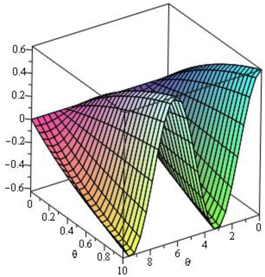
Figure 1. Behavior of q-HAGTM solution $\xi (\vartheta ,\theta )$ for diffusion Equation (27) when $h=-1,n=1$, and $\mu =1$.

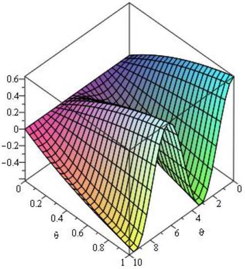
Figure 2. Response of exact solution $\xi (\vartheta ,\theta )$ for diffusion Equation (27) when $h=-1,n=1$, and $\mu =1$.

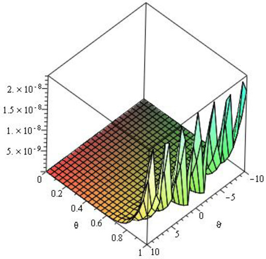
Figure 3. Error between approximate solutions and exact solutions for diffusion Equation (27) when $h=-1,n=1$, and $\mu =1$.

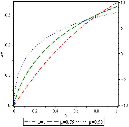
Figure 4. Behavior of q-HAGTM solution $\xi (\vartheta ,\theta )$ of diffusion Equation (27) for diverse values of $\mu$ at $\vartheta =1$.

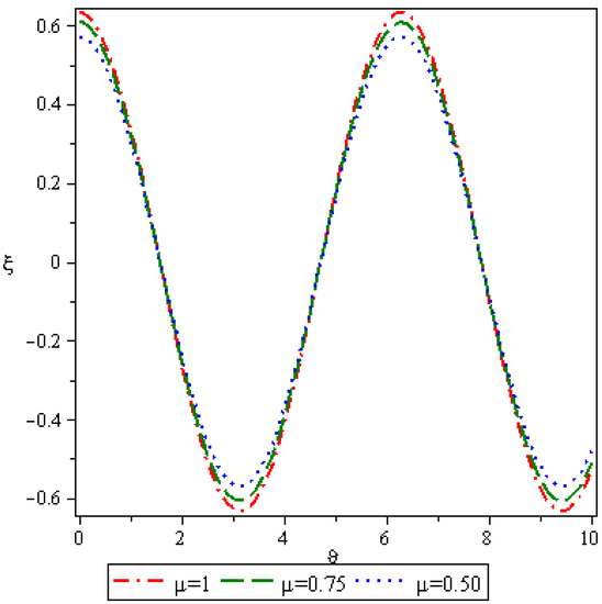
Figure 5. q-HAGTM solution $\xi (\vartheta ,\theta )$ of diffusion Equation (27) for several values of fractional order $\mu$ at $\theta =1$.

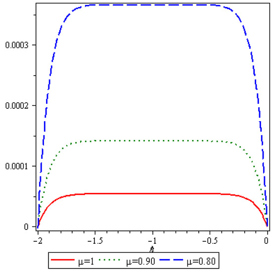
Figure 6. Curve of diffusion of Equation (27) for numerous values of order $\mu$.

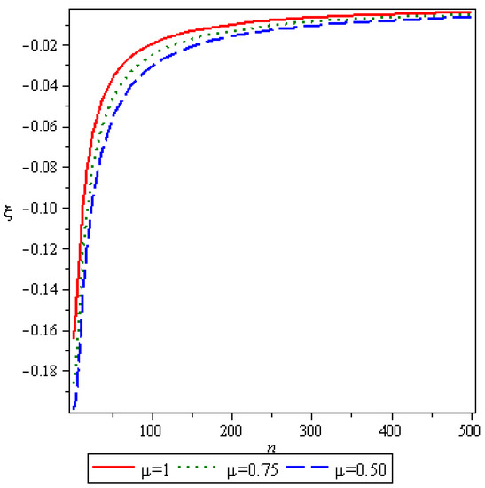
Figure 7. Curve of diffusion of Equation (27) for several values of order $\mu$.

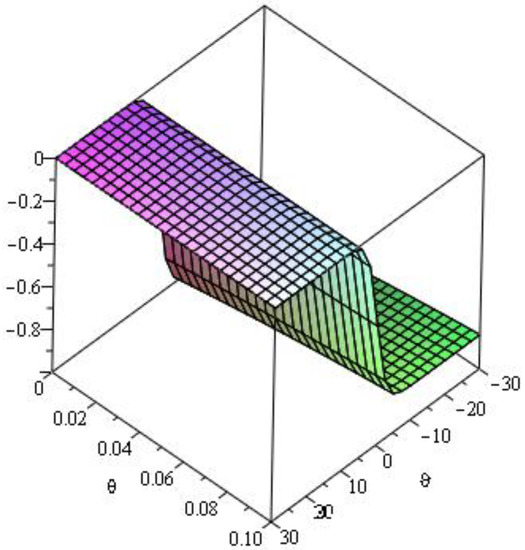
Figure 8. Characteristic of q-HAGTM solution $\xi (\vartheta ,\theta )$ for AC Equation (41) when $h=-1,n=1$, and $\mu =1$.

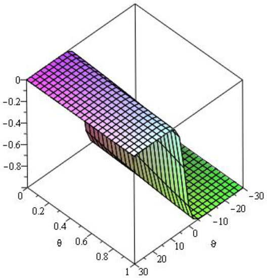
Figure 9. Exact solution $\xi (\vartheta ,\theta )$ for AC Equation (41) when $h=-1,n=1$, and $\mu =1$.

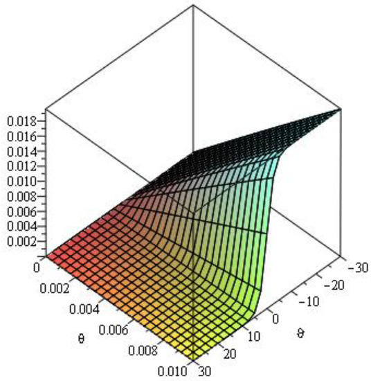
Figure 10. Error between approximate solutions and exact solutions for AC Equation (41) when $h=-1,n=1$, and $\mu =1$.

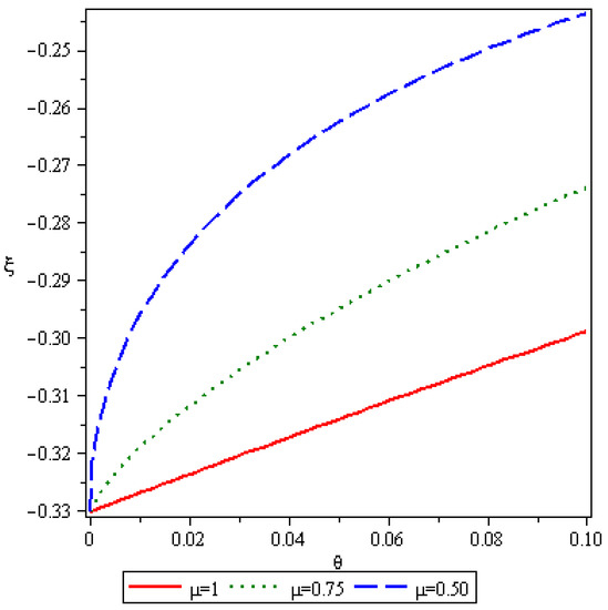
Figure 11. Response of q-HAGTM solution $\xi (\vartheta ,\theta )$ for AC Equation (41) for numerous values of order $\mu$ at $\vartheta =1$.

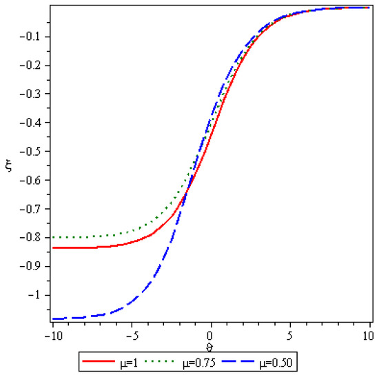
Figure 12. Characteristic of q-HAGTM solution $\xi (\vartheta ,\theta )$ for AC Equation (41) for diverse values of order $\mu$ at $\theta =0.1$.

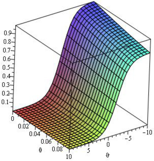
Figure 13. Characteristic of q-HAGTM solution $\xi (\vartheta ,\theta )$ for AC Equation (54) when $h=-1,n=1$, and $\mu =1$.

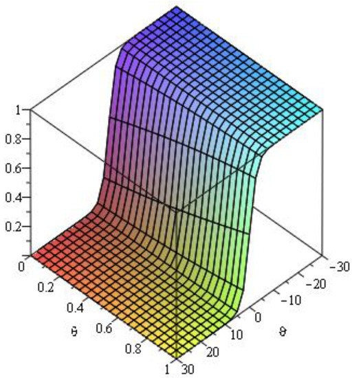
Figure 14. Exact solution $\xi (\vartheta ,\theta )$ for AC Equation (54) when $h=-1,n=1$, and $\mu =1$.

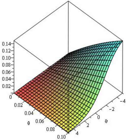
Figure 15. Error between approximate solutions and exact solutions for AC Equation (54) when $h=-1,n=1$, and $\mu =1$.

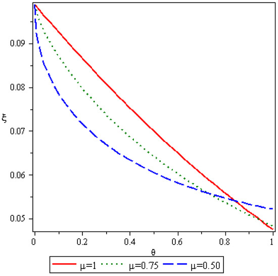
Figure 16. q-HAGTM solution $\xi (\vartheta ,\theta )$ for AC Equation (54) for various values of order $\mu$ at $\vartheta =1$.

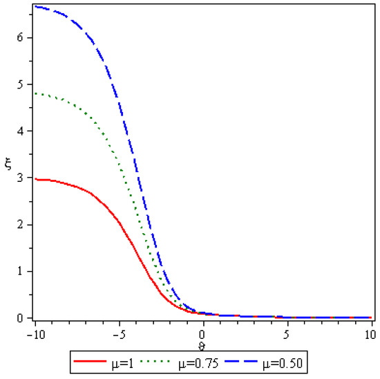
Figure 17. Response of q-HAGTM solution $\xi (\vartheta ,\theta )$ for AC Equation (54) for different values of fractional order $\mu$ at $\theta =1$.

6. Conclusions

In this article, to study the characteristic of diffusion equation and AC equation occurring in oil pollution associated with the Caputo–Katugampola derivative, an effective technique, namely, q-HAGTM has been proposed. By analyzing numerical results and graphical simulations, we observe that q-HAGTM is successfully applied to solve the diffusion equation and AC equation pertaining to the Caputo–Katugampola derivative. The displacement imparts an advanced characteristic for fractional order derivative comparing to classical order derivative. Hence, it is concluded that the employed technique is very efficient, accurate, and can be applied to analyze a wide category of fractional order models appearing in oil pollution.

References

- Miller, K.S.; Ross, B. An Introduction to the Fractional Calculus and Fractional Differential Equations; Willey: New York, NY, USA, 1993. [Google Scholar]
- Podlubny, I. Fractional Differential Equations; Academic Press: San Diego, CA, USA, 1999; Volume 198, p. 340. [Google Scholar]
- Caputo, M. Elasticita e Dissipazione; Zani-Chelli: Bologna, Italy, 1969. [Google Scholar]
- Singh, J. Analysis of fractional blood alcohol model with composite fractional derivative. Chaos Solitons Fractals 2020, 140, 110127. [Google Scholar] [CrossRef]
- Caputo, M.; Fabrizio, M. A new definition of fractional derivative without singular kernel. Progr. Fract. Differ. Appl. 2015, 1, 73–85. [Google Scholar]
- Caputo, M.; Fabrizio, M. On the Singular Kernels for Fractional Derivatives. Some Applications to Partial Differential Equations. Progr. Fract. Differ. Appl. 2021, 7, 79–82. [Google Scholar]
- Singh, J.; Kumar, D.; Kumar, S. An efficient computational method for local fractional transport equation occurring in fractal porous media. Comput. Appl. Math. 2020, 39, 137. [Google Scholar] [CrossRef]
- Singh, J.; Ahmadian, A.; Sushila; Kumar, D.; Baleanu, D.; Senu, N. An Efficient Computational Approach for Local Fractional Poisson Equation in Fractal Media. Numer. Methods Partial. Differ. Equ. 2020, 37, 1439–1448. [Google Scholar] [CrossRef]
- Yang, X.J. A new integral transform operator for solving the heat-diffusion problem. Appl. Math. Lett. 2017, 64, 193–197. [Google Scholar] [CrossRef]
- Losada, J.; Nieto, J.J. Properties of the new fractional derivative without singular kernel. Progr. Fract. Differ. Appl. 2015, 1, 87–92. [Google Scholar]
- Atangana, A.; Baleanu, D. New fractional derivative with nonlocal and non-singular kernel, Theory and application to heat transfer model. Therm. Sci. 2016, 20, 763–769. [Google Scholar] [CrossRef]
- Kumar, D.; Agarwal, R.P.; Singh, J. A modified numerical scheme and convergence analysis for fractional model of Lienard’s equation. J. Comput. Appl. Math. 2018, 339, 405–413. [Google Scholar] [CrossRef]
- Hariharan, G. An efficient Legendre wavelet-based approximation method for a few Newell-Whitehead and Allen-Cahn equations. J. Membr. Biol. 2014, 247, 371–380. [Google Scholar] [CrossRef] [PubMed]
- Allen, S.M.; Cahn, J.W. A microscopic theory for antiphase boundary motion and its application to antiphase domain coarsening. Acta Metall. 1979, 27, 1085–1095. [Google Scholar] [CrossRef]
- Shah, A.; Sabir, M.; Qasim, M.; Bastian, P. Efficient numerical scheme for solving the Allen-Cahn equation. Numer. Methods Partial. Differ. Equ. 2018, 34, 1820–1833. [Google Scholar] [CrossRef]
- Chen, Y.; Huang, Y.; Yi, N. A SCR-based error estimation and adaptive finite element method for the Allen–Cahn equation. Comput. Math. Appl. 2019, 78, 204–223. [Google Scholar] [CrossRef]
- Ahmad, H.; Khan, T.A.; Durur, H.; Ismail, G.M.; Yokus, A. Analytic approximate solutions of diffusion equations arising in oil pollution. J. Ocean. Eng. Sci. 2021, 6, 62–69. [Google Scholar] [CrossRef]
- Bulut, H.; Atas, S.S.; Baskonus, H.M. Some novel exponential function structures to the Cahn–Allen equation. Cogent Phys. 2016, 3, 1240886. [Google Scholar] [CrossRef]
- Manafian, J. An optimal Galerkin-homotopy asymptotic method applied to the nonlinear second order bvps. Proc. Instit. Math. Mech. 2021, 447, 156–182. [Google Scholar] [CrossRef]
- Shahriari, M.; Manafian, J. An efficient algorithm for solving the fractional dirac differential operator. Adv. Math. Model. Appl. 2020, 5, 289–297. [Google Scholar]
- Dehghan, M.; Manafian, J.; Saadatmandi, A. Solving nonlinear fractional partial differential equations using the homotopy analysis method. Num. Meth. Part. D. E. 2010, 26, 448–479. [Google Scholar] [CrossRef]
- Almeida, R.; Malinowska, A.B.; Odzijewicz, T. Fractional differential equations with dependence on the Caputo-Katugampola derivative. J. Comput. Nonlinear Dynam. 2016, 11, 061017. [Google Scholar] [CrossRef]
- Liao, S.J. Beyond Perturbation: Introduction to Homotopy Analysis Method; Chapman and Hall/CRC Press: Boca Raton, FL, USA, 2003. [Google Scholar]
- Liao, S.J. On the homotopy analysis method for nonlinear problems. Appl. Math. Comput. 2004, 147, 499–513. [Google Scholar] [CrossRef]
- El-Tawil, M.A.; Huseen, S.N. The q-homotopy analysis method (q-HAM). Int. J. App. Math. Mech. 2012, 8, 51–75. [Google Scholar]
- El-Tawil, M.A.; Huseen, S.N. On convergence of the q-homotopy analysis method. Int. J. Contem. Math. Sci. 2013, 8, 481–497. [Google Scholar] [CrossRef]
- Odibat, Z.; Bataineh, S.A. An adaptation of homotopy analysis method for reliable treatment of strongly nonlinear problems: Construction of homotopy polynomials. Math. Meth. Appl. Sci. 2014, 38, 991–1000. [Google Scholar] [CrossRef]
- Singh, J.; Gupta, A.; Baleanu, D. On the analysis of an analytical approach for fractional Caudrey-Dodd-Gibbon equations. Alex. Eng. J. 2021, 61, 5073–5082. [Google Scholar] [CrossRef]
- Singh, J.; Ganbari, B.; Kumar, D.; Baleanu, D. Analysis of fractional model of guava for biological pest control with memory effect. J. Adv. Res. 2021, 32, 99–108. [Google Scholar] [CrossRef] [PubMed]
- Thanompolkrang, S.; Sawangtong, W.; Sawangtong, P. Application of the Generalized Laplace Homotopy Perturbation Method to the Time Fractional Black–Scholes Equations Based on the Katugampola Fractional Derivative in Caputo Type. Computation 2021, 9, 33. [Google Scholar] [CrossRef]
- Jarad, F.; Abdeljawad, T.; Baleanu, D. Caputo-type modification of the Hadamard fractional derivatives. Adv. Differ. Equ. 2012, 142, 1–8. [Google Scholar] [CrossRef]
- Jarad, F.; Abdeljawad, T. Generalized fractional derivatives and Laplace transform. Disc. Cont. Dyn. Syst. S 2019, 13, 709–722. [Google Scholar] [CrossRef]
- Jarad, F.; Abdeljawad, T. A modified Laplace transform for certain generalized fractional operators. Res. Nonlinear Anal. 2018, 2, 88–98. [Google Scholar]
- Katugampola, U.N. New approach to a generalized fractional integral. Appl. Math. Comput. 2011, 218, 860–865. [Google Scholar] [CrossRef]
- Katugampola, U.N. A new approach to generalized fractional derivatives. Bull. Math. Anal. Appl. 2014, 6, 1–15. [Google Scholar]
Publisher’s Note: MDPI stays neutral with regard to jurisdictional claims in published maps and institutional affiliations. |
© 2022 by the authors. Licensee MDPI, Basel, Switzerland. This article is an open access article distributed under the terms and conditions of the Creative Commons Attribution (CC BY) license (https://creativecommons.org/licenses/by/4.0/).