Time-Optimal Control Problem of Two Non-Synchronous Oscillators

Abstract

The time-optimal control problem for a system consisting of two non-synchronous oscillators is considered. Each oscillator is controlled with a shared limited scalar control. The objective of the control is to accelerate the oscillatory system to a given specific position, where the first oscillator must have non-zero phase coordinates, but the second one must remain motionless at the terminal moment. For an arbitrary number of unknown switching moments that determine the optimal relay control, the necessary extremum conditions in the form of nonlinear matrix equalities are proposed. The study of the necessary/sufficient conditions of the extremum made it possible to describe the reachability set in the phase space of the first oscillator, to find an analytical form of the curve corresponding to the two-switching control class, which also separates the reachability set of the three switching-control class. The corresponding theorems are proved and the dependence of the criteria on control constraints is shown. Matrix conditions for different classes of control switchings are found. All of the obtained analytical results are numerically validated and illustrated with mathematical modeling.

1. Introduction

Problems surrounding the lack of control resources (when the dimensions of a control vector are less than the dimensions of the state space of a physically-controlled system) have widespread applications in practice. Oscillatory systems, such as electric circuits [1], mechanical systems [2,3], quantum oscillators [4,5], systems involving physical nature [6,7], and controlled with one external force, are instances of such systems. Using the oscillatory system, it is possible to investigate periodic solutions and the stability of the model of two coupled oscillators in the optics of chiral molecules [6], as well as consider the behaviors of biologically complex mechanisms [7]. Increasing the number of oscillators in these models to sufficiently large N makes it possible to study (analytically and numerically) the macro-parameters and properties of similar systems [8,9].

Thus, the Timoshenko–Ehrenfest beam motion control, which is modeled with a system of N oscillators that perform forced oscillations under the actions of scalar and limited control forces, was considered in work [2]. The time-optimal problem for a platform with attached oscillators was investigated in [3]. The maximum variation of the oscillation energy of the oscillator system for a given time was examined in [10]. Due to the difficulties in finding an analytical solution for the control problems, it is of interest to asymptotically synthesize the optimal control of a system of an arbitrary number of linear oscillators (with general limited control), as obtained in [11].

Optimal control problems were investigated using the Pontryagin maximum principle, which was formulated during the seminars on the theory of oscillations and automatic control by L.S. Pontryagin and M.A. Aizerman in the 1950s, where the problem of optimal performance was considered [12]. For systems considered in [1,5], it is often necessary for one of the subsystems to get into the required position as quickly as possible, while the others should remain at rest at the terminal moment. Thus, for a single oscillator, V.G. Boltyansky obtained the synthesis of optimal control in the time-optimal problem [13]. The optimal control problems for the systems of many oscillators with various criteria have already been studied by F.L. Chernousko in [14], where a significant complexity of obtaining an analytical solution was noted, and the problem involving two oscillators was solved for a very special case of their frequency ratio.

In this paper, we review the time-optimal control problem for two non-synchronous oscillators controlled by limited scalar impacts with initial zero-phase coordinates but different terminal ones, which are features of the problem statement that considerably complicate it.

One of the key aspects of such control problems is the study of the accessibility and controllability of the oscillatory system [15]. It can be shown with the methods of geometric control theory [16], namely: the Sussman–Djurdjevic and the Poincare theorems, as well as with the results of the classical optimal control theory, the La Salle–Conti theorem [17].

This article is structured as follows. In Section 2, the optimal control problem is formulated. In Section 3, the optimal control law is presented using the Pontryagin maximum principle. Section 4 examines the necessary and sufficient optimality conditions for different classes of control switchings. Section 5 discusses the continuity of the problem criterion on the control parameter. Section 6 illustrates the obtained results, in particular, the mathematical modeling of the set of reachability of the first oscillator, the criterion of the problem, and the time intervals of the switching controls. In the conclusion, we suggest directions for further research.

2. Optimal Control Problem Statement

A system consisting of two non-synchronous oscillators, i.e., having different natural frequencies $({\omega }_1\ne {\omega }_2)$, was considered. The control $u\left(t\right)$ impacts the momenta $p_1,p_2$ of both oscillators, but not their coordinates $q_1,q_2$. The motion of this linear control system is described with the following system of equations:

$$\left\{\begin{array}{c}{\dot{q}}_1\left(t\right)=p_1\left(t\right),\hfill \\ {\dot{p}}_1\left(t\right)=-{\omega }_1^2{q}_1\left(t\right)+u\left(t\right),\hfill \\ {\dot{q}}_2\left(t\right)=p_2\left(t\right),\hfill \\ {\dot{p}}_2\left(t\right)=-{\omega }_2^2{q}_2\left(t\right)+u\left(t\right),\hfill \end{array}\right.x={(q_1,p_1,q_2,p_2)}^T\in {\mathbb{R}}^4=M.$$

(1)

The system (1) can be rewritten in matrix form $\dot{x}\left(t\right)=Ax\left(t\right)+Bu\left(t\right)$, where

$${\displaystyle A=\left(\begin{array}{cccc}0& 1& 0& 0\\ -{\omega }_1^2& 0& 0& 0\\ 0& 0& 0& 1\\ 0& 0& -{\omega }_2^2& 0\end{array}\right),B=\left(\begin{array}{c}0\\ 1\\ 0\\ 1\end{array}\right).}$$

The number of non-zero components of the control vector B is less than the dimensionality of the system; moreover, the control is limited by a value $\epsilon$, which is a parameter of the problem:

$$u\left(t\right)\in [-\epsilon ,\epsilon ]=U.$$

(2)

At the initial moment, the phase states of both oscillators coincide with the origins of the phase coordinate planes, i.e., their coordinates and momenta are equal to zero. At the terminal moment, the phase coordinates of the second oscillator become zero again, while the first oscillator moves to the state $(q_1^{T_0},p_1^{T_0})$, which are also parameters of the problem. The explicit forms of the initial and terminal conditions are

$$x\left(0\right)=x_0={(0,0,0,0)}^T,$$

(3)

$$x\left(T_0\right)=x_{T_0}={(q_1^{T_0},p_1^{T_0},0,0)}^T,$$

(4)

where $T_0$ is a terminal moment and T defines a transpose operation.

The total time of the system’s movement from the initial state to the terminal one is chosen as the criterion of the problem and needs to be minimized:

$${\displaystyle T_0\left[u\right]={\int }_0^{T_0}dt\to \underset{u(·)\in U}{min}.}$$

(5)

The proofs of global controllability and strong accessibility of the system (1) with the condition (2) are given in [15,18].

3. Solution of the Optimal Control Problem

To investigate and solve problems (1)–(5), the Pontryagin maximum principle (PMP) is used. The maximum principles in the canonical coordinates consist of the following statements:

• The Hamiltonian for the optimal control problem is expressed as

  $${\displaystyle h_u=-{\lambda }_0+{\xi }_1{p}_1+{\xi }_2{p}_2+{\eta }_1(-{\omega }_1^2{q}_1+u)+{\eta }_2(-{\omega }_2^2{q}_2+u),{\lambda }_0>0,}$$

  (6)

  where ${\xi }_1,{\xi }_2,{\eta }_1,{\eta }_2$ are adjoint variables and ${\lambda }_0$ is constant.
• A Hamiltonian system, including motion equations and an adjoint system of equations:

  $$\left\{\begin{array}{c}{\dot{q}}_1\left(t\right)=p_1\left(t\right),\hfill \\ {\dot{p}}_1\left(t\right)=-{\omega }_1^2{q}_1\left(t\right)+u\left(t\right),\hfill \\ {\dot{q}}_2\left(t\right)=p_2\left(t\right),\hfill \\ {\dot{p}}_2\left(t\right)=-{\omega }_2^2{q}_2\left(t\right)+u\left(t\right),\hfill \end{array}\right.\left\{\begin{array}{c}{\displaystyle {\dot{\xi }}_1\left(t\right)=-\frac{\partial h_u}{\partial q_1}={\omega }_1^2{\eta }_1\left(t\right),}\hfill \\ {\displaystyle {\dot{\eta }}_1\left(t\right)=-\frac{\partial h_u}{\partial p_1}=-{\xi }_1\left(t\right),}\hfill \\ {\displaystyle {\dot{\xi }}_2\left(t\right)=-\frac{\partial h_u}{\partial q_2}={\omega }_2^2{\eta }_2\left(t\right),}\hfill \\ {\displaystyle {\dot{\eta }}_2\left(t\right)=-\frac{\partial h_u}{\partial p_2}=-{\xi }_2\left(t\right).}\hfill \end{array}\right.$$

  (7)
• Maximum condition

  $${\displaystyle h_{u^{\ast }}=\underset{u(·)\in U}{max}{h}_u=-{\lambda }_0+{\xi }_1{p}_1+{\xi }_2{p}_2-{\eta }_1{\omega }_1^2{q}_1-{\eta }_2{\omega }_2^2{q}_2+u^{\ast }({\eta }_1+{\eta }_2).}$$

  (8)

Transversality conditions are absent because the optimal problem statement involves fixed endpoints.

The Hamiltonian (8) is linear with respect to $u^{\ast }$ and, thus, the optimal control is given by the bang–bang control: $u^{\ast }=-\epsilon$ for ${\eta }_1+{\eta }_2<0$ and $u^{\ast }=\epsilon$ for ${\eta }_1+{\eta }_2>0$, which can be written as

$$u^{\ast }\left(t\right)=\epsilon sign\left(SF\left(t\right)\right),$$

(9)

$$SF\left(t\right)={\eta }_1\left(t\right)+{\eta }_2\left(t\right),$$

(10)

where $SF\left(t\right)$ is a switching function. The adjoint system can be rewritten in the following form

$$\left\{\begin{array}{c}{\displaystyle {\ddot{\eta }}_1\left(t\right)=-{\omega }_1^2{\eta }_1\left(t\right),}\hfill \\ {\displaystyle {\ddot{\eta }}_2\left(t\right)=-{\omega }_2^2{\eta }_2\left(t\right).}\hfill \end{array}\right.$$

(11)

From the system (11) ${\eta }_1\left(t\right)$ and ${\eta }_2\left(t\right)$ can be found:

$$\begin{array}{c}{\eta }_1\left(t\right)=C_{1}cos\left({\omega }_{1}t\right)+C_{2}sin\left({\omega }_{1}t\right),\hfill \\ {\eta }_2\left(t\right)=C_{3}cos\left({\omega }_{2}t\right)+C_{4}sin\left({\omega }_{2}t\right),\hfill \end{array}$$

(12)

where ${\displaystyle C=\left(\begin{array}{cccc}{C}_1,& C_2,& C_3,& C_4\end{array}\right)}$ is a constant vector. Combining the expressions (9) and (12), an explicit form of the optimal control law can be obtained

$${\displaystyle u^{\ast }\left(t\right)=\epsilon sign(C_{1}cos\left({\omega }_{1}t\right)+C_{2}sin\left({\omega }_{1}t\right)+C_{3}cos\left({\omega }_{2}t\right)+C_{4}sin\left({\omega }_{2}t\right)).}$$

(13)

This function is uniquely defined and cannot be equal to zero on the whole interval, perhaps with the exception of the isolated points, which lead to the absence of special control modes.

The relay form of the optimal control obtained in this Section allows explicitly writing solutions of the motion Equation (1) taking into account how many times the control (13) will change the sign and obtain the necessary extremum conditions for any number of such switchings.

4. The Necessary Extremum Conditions

For the relay control (13), two values are defined: the moment of switching $t_i,$$i=\overline{1,K-1}$, $K\in \mathbb{N}$, when the control changes signs and the duration of control intervals ${\tau }_n,n=\overline{1,K}$. Here, a further designation $\overline{1,K}$, which means “$1,2,\dots ,K$”, is used for convenience. The optimal control $u^{\ast }\left(t\right)$ with $K-1$ switchings and K control intervals is illustrated in Figure 1:

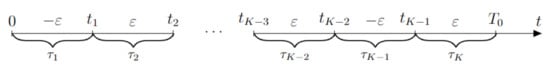
Figure 1. Control intervals for optimal control $u^{\ast }\left(t\right)$.

Definition 1.

The term “$(K-1)$-switching control class” defines an optimal solution where the optimal control has exactly $K-1$ switchings.

The solution to the system of motion Equation (1) with boundary conditions (3) and (4) has a general form

$$\left\{\begin{array}{c}{\displaystyle q_1\left(T_0\right)=\frac{1}{{\omega }_1}{\int }_0^{T_0}sin\left({\omega }_1(T_0-\tau )\right)u\left(\tau \right)d\tau =q_1^{T_0},}\\ \\ {\displaystyle p_1\left(T_0\right)={\int }_0^{T_0}cos\left({\omega }_1(T_0-\tau )\right)u\left(\tau \right)d\tau =p_1^{T_0},}\\ \\ {\displaystyle q_2\left(T_0\right)=\frac{1}{{\omega }_2}{\int }_0^{T_0}sin\left({\omega }_2(T_0-\tau )\right)u\left(\tau \right)d\tau =0,}\\ \\ {\displaystyle p_2\left(T_0\right)={\int }_0^{T_0}cos\left({\omega }_2(T_0-\tau )\right)u\left(\tau \right)d\tau =0.}\end{array}\right.$$

(14)

The structure of optimal control (13) allows to write a solution of the system that takes into account not only the number of switchings $K-1$, but also the sign of the control at the first interval.

$$\left\{\begin{array}{c}{\displaystyle 2\sum _{j=1}^K{(-1)}^{j+1}cos\left({\omega }_1\sum _{i=j}^K{\tau }_i\right)-cos\left({\omega }_1\sum _{i=1}^K{\tau }_i\right)={(-1)}^{K-1}+{(-1)}^{k+1}\frac{q_1^{T_0}{\omega }_1^2}{\epsilon },}\hfill \\ \\ {\displaystyle 2\sum _{j=1}^K{(-1)}^{j+1}sin\left({\omega }_1\sum _{i=j}^K{\tau }_i\right)-sin\left({\omega }_1\sum _{i=1}^K{\tau }_i\right)={(-1)}^k\frac{p_1^{T_0}{\omega }_1}{\epsilon },}\hfill \\ \\ {\displaystyle 2\sum _{j=1}^K{(-1)}^{j+1}cos\left({\omega }_2\sum _{i=j}^K{\tau }_i\right)-cos\left({\omega }_2\sum _{i=1}^K{\tau }_i\right)={(-1)}^{K-1},}\hfill \\ \\ {\displaystyle 2\sum _{j=1}^K{(-1)}^{j+1}sin\left({\omega }_2\sum _{i=j}^K{\tau }_i\right)-sin\left({\omega }_2\sum _{i=1}^K{\tau }_i\right)=0,}\hfill \end{array}\right.$$

(15)

where an additional parameter k equal to 0 or 1 corresponds to the initial control $\epsilon$ and $-\epsilon$, respectively.

Remark 1.

A system (15) consisting of four equations can be used to study the three-switching control class, where four control intervals need to be determined.

The two-switching control class occurs as degeneration of other classes. For example, when the outermost interval is zeroed in on a three-switching control class, or the internal interval is zeroed in on a four-switching control class.

Lemma 1.

In the two-switching control class, the functional dependencies for the duration of the control intervals ${\tau }_1$, ${\tau }_2$, ${\tau }_3$ are valid

$$cos\left({\omega }_2{\tau }_1\right)=cos\left({\omega }_2{\tau }_3\right),$$

$$cos\left({\omega }_2{\tau }_2\right)=\frac{2{cos}^2\left({\omega }_2{\tau }_1\right)-4cos\left({\omega }_2{\tau }_1\right)+3}{5-4cos\left({\omega }_2{\tau }_1\right)}if{\tau }_2<\frac{2\pi }{{\omega }_2}.$$

The proof of Lemma 1 is given in Appendix A.

To investigate control classes with more than three switchings, the necessary extremum conditions are introduced.

Theorem 1

(Necessary Extremum Conditions). Any solution to the problem (1)–(5) in the class of piecewise constant controls (13) satisfies the system (15) and $K-4$ equalities:

$${\displaystyle det\left(\begin{array}{cccc}cos\left({\omega }_1{t}_i\right)& cos\left({\omega }_1{t}_{i+1}\right)& cos\left({\omega }_1{t}_{i+2}\right)& cos\left({\omega }_1{t}_{i+3}\right)\\ sin\left({\omega }_1{t}_i\right)& sin\left({\omega }_1{t}_{i+1}\right)& sin\left({\omega }_1{t}_{i+2}\right)& sin\left({\omega }_1{t}_{i+3}\right)\\ cos\left({\omega }_2{t}_i\right)& cos\left({\omega }_2{t}_{i+1}\right)& cos\left({\omega }_2{t}_{i+2}\right)& cos\left({\omega }_2{t}_{i+3}\right)\\ sin\left({\omega }_2{t}_i\right)& sin\left({\omega }_2{t}_{i+1}\right)& sin\left({\omega }_2{t}_{i+2}\right)& sin\left({\omega }_2{t}_{i+3}\right)\end{array}\right)=0,i=\overline{1,K-4}.}$$

(16)

Proof. 

The switching function (10) that determines the optimal control (13) becomes zero at moments $t_i,i=\overline{1,K-1}$, when control switchings occur:

$${\displaystyle SF\left(t_i\right)=C_{1}cos\left({\omega }_1{t}_i\right)+C_{2}sin\left({\omega }_1{t}_i\right)+C_{3}cos\left({\omega }_2{t}_i\right)+C_{4}sin\left({\omega }_2{t}_i\right)=0,i=\overline{1,K-1}}$$

(17)

For a more compact notation, Equation (17) can be rewritten in matrix form

$${\displaystyle (C,{\mathsf{\Omega }}_i)=0,i=\overline{1,K-1},}$$

(18)

where

$${\displaystyle C=\left(\begin{array}{cccc}{C}_1,& C_2,& C_3,& C_4\end{array}\right),{\mathsf{\Omega }}_i=\left(\begin{array}{c}cos\left({\omega }_1{t}_i\right)\\ sin\left({\omega }_1{t}_i\right)\\ cos\left({\omega }_2{t}_i\right)\\ sin\left({\omega }_2{t}_i\right)\end{array}\right).}$$

Equation (18) form the system consisting of $K-1$ equations

$${\displaystyle {\left(\begin{array}{ccccc}cos\left({\omega }_1{t}_1\right)& cos\left({\omega }_1{t}_2\right)& \dots & cos\left({\omega }_1{t}_{K-2}\right)& cos\left({\omega }_1{t}_{K-1}\right)\\ sin\left({\omega }_1{t}_1\right)& sin\left({\omega }_1{t}_2\right)& \dots & sin\left({\omega }_1{t}_{K-2}\right)& sin\left({\omega }_1{t}_{K-1}\right)\\ cos\left({\omega }_2{t}_1\right)& cos\left({\omega }_2{t}_2\right)& \dots & cos\left({\omega }_2{t}_{K-2}\right)& cos\left({\omega }_2{t}_{K-1}\right)\\ sin\left({\omega }_2{t}_1\right)& sin\left({\omega }_2{t}_2\right)& \dots & sin\left({\omega }_2{t}_{K-2}\right)& sin\left({\omega }_2{t}_{K-1}\right)\end{array}\right)}^T\left(\begin{array}{c}{C}_1\\ C_2\\ C_3\\ C_4\end{array}\right)=\overrightarrow{0}.}$$

(19)

The condition of the existence of the non-zero vector C in (19) is equivalent to $K-4$ equalities

$${\displaystyle det\left({\mathsf{\Omega }}_i,{\mathsf{\Omega }}_{i+1},{\mathsf{\Omega }}_{i+2},{\mathsf{\Omega }}_{i+3}\right)=0,i=\overline{1,K-4}.}$$

(20)

In other words, (20) are the non-degeneracy conditions of vector C, defining the optimal control (13). □

Remark 2.

In the case when $K-1=4$, the condition of the existence of non-zero vector C has the form

$${\displaystyle det\left(\begin{array}{cccc}cos\left({\omega }_1{t}_1\right)& cos\left({\omega }_1{t}_2\right)& cos\left({\omega }_1{t}_3\right)& cos\left({\omega }_1{t}_4\right)\\ sin\left({\omega }_1{t}_1\right)& sin\left({\omega }_1{t}_2\right)& sin\left({\omega }_1{t}_3\right)& sin\left({\omega }_1{t}_4\right)\\ cos\left({\omega }_2{t}_1\right)& cos\left({\omega }_2{t}_2\right)& cos\left({\omega }_2{t}_3\right)& cos\left({\omega }_2{t}_4\right)\\ sin\left({\omega }_2{t}_1\right)& sin\left({\omega }_2{t}_2\right)& sin\left({\omega }_2{t}_3\right)& sin\left({\omega }_2{t}_4\right)\end{array}\right)=0,}$$

(21)

which is equivalent to the following equation

$$\begin{array}{c}{\displaystyle sin\left(w_2{\tau }_4\right)sin\left(w_1{\tau }_2\right)-sin\left(w_2({\tau }_3+{\tau }_4)\right)sin\left(w_1({\tau }_2+{\tau }_3)\right)-sin\left(w_2({\tau }_2+{\tau }_3)\right)sin\left(w_1({\tau }_3+{\tau }_4)\right)+}\hfill \\ {\displaystyle +sin\left(w_2{\tau }_3\right)sin\left(w_1({\tau }_2+{\tau }_3+{\tau }_4)\right)+sin\left(w_2({\tau }_2+{\tau }_3+{\tau }_4)\right)sin\left(w_1{\tau }_3\right)+sin\left(w_2{\tau }_2\right)sin\left(w_1{\tau }_4\right)=0.}\hfill \end{array}$$

(22)

If $K-1>4$, there are ${\mathbf{C}}_{K-1}^4$ (number of permutations) of the non-zero conditions for the vector C

$$\begin{array}{c}{\displaystyle det\left(\begin{array}{cccc}cos\left({\omega }_1{t}_{m_1}\right)& cos\left({\omega }_1{t}_{m_2}\right)& cos\left({\omega }_1{t}_{m_3}\right)& cos\left({\omega }_1{t}_{m_4}\right)\\ sin\left({\omega }_1{t}_{m_1}\right)& sin\left({\omega }_1{t}_{m_2}\right)& sin\left({\omega }_1{t}_{m_3}\right)& sin\left({\omega }_1{t}_{m_4}\right)\\ cos\left({\omega }_2{t}_{m_1}\right)& cos\left({\omega }_2{t}_{m_2}\right)& cos\left({\omega }_2{t}_{m_3}\right)& cos\left({\omega }_2{t}_{m_4}\right)\\ sin\left({\omega }_2{t}_{m_1}\right)& sin\left({\omega }_2{t}_{m_2}\right)& sin\left({\omega }_2{t}_{m_3}\right)& sin\left({\omega }_2{t}_{m_4}\right)\end{array}\right)=0,}\\ \\ m_1\ne m_2\ne m_3\ne m_4;m_1,m_2,m_3,m_4=\overline{1,K-1}.\end{array}$$

(23)

Then, in order to find ${\tau }_i$, it is required to use (15) together with $K-4$ equations from the set (23), so that all the moments of $t_i$ are contained there. A set that satisfies these conditions is (20), for example.

Remark 3.

Theorem 1 allows finding all of the required switching moments $t_i,i=\overline{1,K-1}$ that define vector C as the kernel of the corresponding linear mapping in (19).

This implies another necessary condition of the extremum, which is formulated in the form of the following lemma.

Lemma 2.

The optimal control $u^{\ast }\left(t\right)$ with vector C obtained from (19) contains exactly $K-1$ zeros and, according to Definition 1, corresponds to the $(K-1)$-switching control class.

In the next section, a theorem considering the continuity of the problem criterion from the parameter $\epsilon$ is formulated and proved.

5. Continuity of ${\mathbf{T}}_{\mathbf{0}}\left(\mathbf{\epsilon }\right)$

To find sufficient conditions for the continuity of a function $T_0\left(\epsilon \right)$, the implicit function theorem is applied. Let us write out the Jacobian of a system consisting of equations of motion (15) and additional conditions (16) obtained by Theorem 1 on the necessary extremum conditions.

The equations of the joint system are denoted by $f_1,f_2,\dots ,f_K$, where $f_1,f_2,f_3,f_4$ relate to the equations of motion (15), and $f_5,\dots ,f_K$ are responsible for the non-degeneracy conditions (20). The Jacobian $J_{K-1}$ corresponds to the $(K-1)$-switching control class and consists of partial derivatives of K functions with K variables.

$${\displaystyle J_{K-1}=det\left(\begin{array}{cccc}{\displaystyle \frac{\partial f_1}{\partial \tau {}_1}}& {\displaystyle \frac{\partial f_1}{\partial \tau {}_2}}& \dots & {\displaystyle \frac{\partial f_1}{\partial \tau {}_K}}\\ {\displaystyle \frac{\partial f_2}{\partial \tau {}_1}}& {\displaystyle \frac{\partial f_2}{\partial \tau {}_2}}& \dots & {\displaystyle \frac{\partial f_2}{\partial \tau {}_K}}\\ \dots & \dots & \ddots & \dots \\ {\displaystyle \frac{\partial f_K}{\partial \tau {}_1}}& {\displaystyle \frac{\partial f_K}{\partial \tau {}_2}}& \dots & {\displaystyle \frac{\partial f_K}{\partial \tau {}_K}}\end{array}\right)=}$$

(24)

$${\displaystyle =det\left(\left(\begin{array}{cccc}{\displaystyle -2{\omega }_{1}sin\left({\omega }_1\sum _{i=1}^K{\tau }_i\right)}& {\displaystyle -2{\omega }_1\sum _{j=1}^2-1^{j+1}sin\left({\omega }_1\sum _{i=j}^K{\tau }_i\right)}& \dots & {\displaystyle -2{\omega }_1\sum _{j=1}^K-1^{j+1}sin\left({\omega }_1\sum _{i=j}^K{\tau }_i\right)}\\ {\displaystyle 2{\omega }_{1}cos\left({\omega }_1\sum _{i=1}^K{\tau }_i\right)}& {\displaystyle 2{\omega }_1\sum _{j=1}^2-1^{j+1}cos\left({\omega }_1\sum _{i=j}^K{\tau }_i\right)}& \dots & {\displaystyle 2{\omega }_1\sum _{j=1}^K-1^{j+1}cos\left({\omega }_1\sum _{i=j}^K{\tau }_i\right)}\\ {\displaystyle -2{\omega }_{2}sin\left({\omega }_2\sum _{i=1}^K{\tau }_i\right)}& {\displaystyle -2{\omega }_2\sum _{j=1}^2-1^{j+1}sin\left({\omega }_2\sum _{i=j}^K{\tau }_i\right)}& \dots & {\displaystyle -2{\omega }_2\sum _{j=1}^K-1^{j+1}sin\left({\omega }_2\sum _{i=j}^K{\tau }_i\right)}\\ {\displaystyle 2{\omega }_{2}cos\left({\omega }_2\sum _{i=1}^K{\tau }_i\right)}& {\displaystyle 2{\omega }_2\sum _{j=1}^2-1^{j+1}cos\left({\omega }_2\sum _{i=j}^K{\tau }_i\right)}& \dots & {\displaystyle 2{\omega }_2\sum _{j=1}^K-1^{j+1}cos\left({\omega }_2\sum _{i=j}^K{\tau }_i\right)}\\ {\displaystyle \frac{\partial f_5}{\partial \tau {}_1}}& {\displaystyle \frac{\partial f_5}{\partial \tau {}_2}}& \dots & {\displaystyle \frac{\partial f_5}{\partial \tau {}_K}}\\ \dots & \dots & \ddots & \dots \\ {\displaystyle \frac{\partial f_K}{\partial \tau {}_1}}& {\displaystyle \frac{\partial f_K}{\partial \tau {}_2}}& \dots & {\displaystyle \frac{\partial f_K}{\partial \tau {}_K}}\end{array}\right)+\right.}$$

$${\displaystyle +\left.\left(\begin{array}{cccc}{\displaystyle {\omega }_{1}sin\left({\omega }_1\sum _{i=1}^K{\tau }_i\right)}& {\displaystyle {\omega }_{1}sin\left({\omega }_1\sum _{i=1}^K{\tau }_i\right)}& \dots & {\displaystyle {\omega }_{1}sin\left({\omega }_1\sum _{i=1}^K{\tau }_i\right)}\\ {\displaystyle -{\omega }_{1}cos\left({\omega }_1\sum _{i=1}^K{\tau }_i\right)}& {\displaystyle -{\omega }_{1}cos\left({\omega }_1\sum _{i=1}^K{\tau }_i\right)}& \dots & {\displaystyle -{\omega }_{1}cos\left({\omega }_1\sum _{i=1}^K{\tau }_i\right)}\\ {\displaystyle {\omega }_{2}sin\left({\omega }_2\sum _{i=1}^K{\tau }_i\right)}& {\displaystyle {\omega }_{2}sin\left({\omega }_2\sum _{i=1}^K{\tau }_i\right)}& \dots & {\displaystyle {\omega }_{2}sin\left({\omega }_2\sum _{i=1}^K{\tau }_i\right)}\\ {\displaystyle -{\omega }_{2}cos\left({\omega }_2\sum _{i=1}^K{\tau }_i\right)}& {\displaystyle -{\omega }_{2}cos\left({\omega }_2\sum _{i=1}^K{\tau }_i\right)}& \dots & {\displaystyle -{\omega }_{2}cos\left({\omega }_2\sum _{i=1}^K{\tau }_i\right)}\\ 0& 0& \dots & 0\\ \dots & \dots & \ddots & \dots \\ 0& 0& \dots & 0\end{array}\right)\right).}$$

Let us transform the above determinant, leading the Jacobian to a simpler form. The determinant of the system will not change if the previous column is subtracted from each column, except for the first.

$${\displaystyle J_{K-1}=det\left(\begin{array}{cccc}{\displaystyle -{\omega }_{1}sin\left({\omega }_1\sum _{i=1}^K{\tau }_i\right)}& {\displaystyle 2{\omega }_{1}sin\left({\omega }_1\sum _{i=2}^K{\tau }_i\right)}& \dots & {\displaystyle -2{\omega }_1{(-1)}^{K+1}sin\left({\omega }_1{\tau }_K\right)}\\ {\displaystyle {\omega }_{1}cos\left({\omega }_1\sum _{i=1}^K{\tau }_i\right)}& {\displaystyle -2{\omega }_{1}cos\left({\omega }_1\sum _{i=2}^K{\tau }_i\right)}& \dots & {\displaystyle 2{\omega }_1{(-1)}^{K+1}cos\left({\omega }_1{\tau }_K\right)}\\ {\displaystyle -{\omega }_{2}sin\left({\omega }_2\sum _{i=1}^K{\tau }_i\right)}& {\displaystyle 2{\omega }_{2}sin\left({\omega }_2\sum _{i=2}^K{\tau }_i\right)}& \dots & {\displaystyle -2{\omega }_2{(-1)}^{K+1}sin\left({\omega }_2{\tau }_K\right)}\\ {\displaystyle {\omega }_{2}cos\left({\omega }_2\sum _{i=1}^K{\tau }_i\right)}& {\displaystyle -2{\omega }_{2}cos\left({\omega }_2\sum _{i=2}^K{\tau }_i\right)}& \dots & {\displaystyle 2{\omega }_2{(-1)}^{K+1}cos\left({\omega }_2{\tau }_K\right)}\\ {\displaystyle \frac{\partial f_5}{\partial {\tau }_1}}& {\displaystyle \frac{\partial f_5}{\partial {\tau }_2}-\frac{\partial f_5}{\partial \tau {}_1}}& \dots & {\displaystyle \frac{\partial f_5}{\partial {\tau }_K}-\frac{\partial f_5}{\partial {\tau }_{K-1}}}\\ \dots & \dots & \ddots & \dots \\ {\displaystyle \frac{\partial f_K}{\partial {\tau }_1}}& {\displaystyle \frac{\partial f_K}{\partial {\tau }_2}-\frac{\partial f_K}{\partial {\tau }_1}}& \dots & {\displaystyle \frac{\partial f_K}{\partial {\tau }_K}-\frac{\partial f_K}{\partial {\tau }_{K-1}}}\end{array}\right).}$$

After multiplying the first and third rows of the resulting matrix by −1 and then replacing the sign for each even column, the transformed Jacobian has the following form

$${\displaystyle J_{K-1}={(-1)}^{\left[\frac{K}{2}\right]}8{\omega }_1^2{\omega }_2^{2}det\left(\begin{array}{cccc}{\displaystyle sin\left({\omega }_1\sum _{i=1}^K{\tau }_i\right)}& {\displaystyle sin\left({\omega }_1\sum _{i=2}^K{\tau }_i\right)}& \dots & {\displaystyle sin\left({\omega }_1{\tau }_K\right)}\\ {\displaystyle cos\left({\omega }_1\sum _{i=1}^K{\tau }_i\right)}& {\displaystyle cos\left({\omega }_1\sum _{i=2}^K{\tau }_i\right)}& \dots & {\displaystyle cos\left({\omega }_1{\tau }_K\right)}\\ {\displaystyle sin\left({\omega }_2\sum _{i=1}^K{\tau }_i\right)}& {\displaystyle sin\left({\omega }_2\sum _{i=2}^K{\tau }_i\right)}& \dots & {\displaystyle sin\left({\omega }_2{\tau }_K\right)}\\ {\displaystyle cos\left({\omega }_2\sum _{i=1}^K{\tau }_i\right)}& {\displaystyle cos\left({\omega }_2\sum _{i=2}^K{\tau }_i\right)}& \dots & {\displaystyle cos\left({\omega }_2{\tau }_K\right)}\\ {\displaystyle 2\frac{\partial f_5}{\partial {\tau }_1}}& {\displaystyle -\frac{\partial f_5}{\partial {\tau }_2}+\frac{\partial f_5}{\partial \tau {}_1}}& \dots & {\displaystyle {(-1)}^{K+1}\left(\frac{\partial f_5}{\partial {\tau }_K}-\frac{\partial f_5}{\partial {\tau }_{K-1}}\right)}\\ \dots & \dots & \ddots & \dots \\ {\displaystyle 2\frac{\partial f_K}{\partial {\tau }_1}}& {\displaystyle -\frac{\partial f_K}{\partial {\tau }_2}+\frac{\partial f_K}{\partial {\tau }_1}}& \dots & {\displaystyle {(-1)}^{K+1}\left(\frac{\partial f_K}{\partial {\tau }_K}-\frac{\partial f_K}{\partial {\tau }_{K-1}}\right)}\end{array}\right).}$$

(25)

The Jacobian, according to Equation (25), for the three-switching control class is written as follows

$${\displaystyle J_3=8{\omega }_1^2{\omega }_2^{2}det\left(\begin{array}{cccc}{\displaystyle sin\left({\omega }_1({\tau }_1+{\tau }_2+{\tau }_3+{\tau }_4)\right)}& {\displaystyle sin\left({\omega }_1({\tau }_2+{\tau }_3+{\tau }_4)\right)}& sin\left({\omega }_1({\tau }_3+{\tau }_4)\right)& {\displaystyle sin\left({\omega }_1{\tau }_4\right)}\\ {\displaystyle cos\left({\omega }_1({\tau }_1+{\tau }_2+{\tau }_3+{\tau }_4)\right)}& {\displaystyle cos\left({\omega }_1({\tau }_2+{\tau }_3+{\tau }_4)\right)}& cos\left({\omega }_1({\tau }_3+{\tau }_4)\right)& {\displaystyle cos\left({\omega }_1{\tau }_4\right)}\\ {\displaystyle sin\left({\omega }_2({\tau }_1+{\tau }_2+{\tau }_3+{\tau }_4)\right)}& {\displaystyle sin\left({\omega }_2({\tau }_2+{\tau }_3+{\tau }_4)\right)}& sin\left({\omega }_2({\tau }_3+{\tau }_4)\right)& {\displaystyle sin\left({\omega }_2{\tau }_4\right)}\\ {\displaystyle cos\left({\omega }_2({\tau }_1+{\tau }_2+{\tau }_3+{\tau }_4)\right)}& {\displaystyle cos\left({\omega }_2({\tau }_2+{\tau }_3+{\tau }_4)\right)}& cos\left({\omega }_2({\tau }_3+{\tau }_4)\right)& {\displaystyle cos\left({\omega }_2{\tau }_4\right)}\end{array}\right).}$$

(26)

The expression (26) has an explicit form

$$\begin{array}{c}{\displaystyle \frac{J_3}{8{\omega }_1^2{\omega }_2^2}=sin\left(w_2{\tau }_3\right)sin\left(w_1{\tau }_1\right)-sin\left(w_2({\tau }_2+{\tau }_3)\right)sin\left(w_1({\tau }_1+{\tau }_2)\right)-}\hfill \\ -sin\left(w_2({\tau }_1+{\tau }_2)\right)sin\left(w_1({\tau }_2+{\tau }_3)\right)+sin\left(w_2{\tau }_2\right)sin\left(w_1({\tau }_1+{\tau }_2+{\tau }_3)\right)+\hfill \\ +sin\left(w_2({\tau }_1+{\tau }_2+{\tau }_3)\right)sin\left(w_1{\tau }_2\right)+sin\left(w_2{\tau }_1\right)sin\left(w_1{\tau }_3\right).\hfill \end{array}$$

(27)

Expressions (21) and (26) can be compared, or rather their explicit forms (22) and (27), respectively. It turns out that with an index shift by one at ${\tau }_i$, the functional parts of these expressions are equal. Expression (26) includes four control intervals in the three-switching class and Expression (21) includes five intervals in the four-switching class, where the first control interval becomes zero at the boundary value $\epsilon$, and that is how the transition into the three-switching class occurs.

This result is derived from several interrelated observations. The first four lines of the Jacobian (25), ordered by cos, sin, and ${\omega }_1$, ${\omega }_2$, which obviously do not change the sign of the determinants, can be written as

$$S_{4,K}=\begin{array}{c}{\displaystyle \left(\begin{array}{cccc}{\displaystyle cos\left({\omega }_1{T}_0\right)}& {\displaystyle cos\left({\omega }_1(T_0-t_1)\right)}& \dots & {\displaystyle cos\left({\omega }_1(T_0-t_{K-1})\right)}\\ sin\left({\omega }_1{T}_0\right)& {\displaystyle sin\left({\omega }_1(T_0-t_1)\right)}& \dots & {\displaystyle sin\left({\omega }_1(T_0-t_{K-1})\right)}\\ {\displaystyle cos\left({\omega }_2{T}_0\right)}& {\displaystyle cos\left({\omega }_2(T_0-t_1)\right)}& \dots & {\displaystyle cos\left({\omega }_2(T_0-t_{K-1})\right)}\\ sin\left({\omega }_2{T}_0\right)& {\displaystyle sin\left({\omega }_2(T_0-t_1)\right)}& \dots & {\displaystyle sin\left({\omega }_2(T_0-t_{K-1})\right)}\end{array}\right)=({\mathsf{\Gamma }}_0,{\mathsf{\Gamma }}_1,\cdots ,{\mathsf{\Gamma }}_{K-1})}\hfill \end{array}$$

(28)

and then converted to the form

$$S_{4,K}=\begin{array}{c}{\displaystyle \left(\begin{array}{c}\left({\displaystyle \begin{array}{cc}cos\left({\omega }_1{T}_0\right)& sin\left({\omega }_1{T}_0\right)\\ sin\left({\omega }_1{T}_0\right)& -cos\left({\omega }_1{T}_0\right)\end{array}}\right)\left({\displaystyle \begin{array}{cccc}{\displaystyle 1}& {\displaystyle cos\left({\omega }_1{t}_1\right)}& \dots & {\displaystyle cos\left({\omega }_1{t}_{K-1}\right)}\\ 0& {\displaystyle sin\left({\omega }_1{t}_1\right)}& \dots & {\displaystyle sin\left({\omega }_1{t}_{K-1}\right)}\end{array}}\right)\\ \left({\displaystyle \begin{array}{cc}cos\left({\omega }_2{T}_0\right)& sin\left({\omega }_2{T}_0\right)\\ sin\left({\omega }_2{T}_0\right)& -cos\left({\omega }_2{T}_0\right)\end{array}}\right)\left({\displaystyle \begin{array}{cccc}{\displaystyle 1}& {\displaystyle cos\left({\omega }_2{t}_1\right)}& \dots & {\displaystyle cos\left({\omega }_2{t}_{K-1}\right)}\\ 0& {\displaystyle sin\left({\omega }_2{t}_1\right)}& \dots & {\displaystyle sin\left({\omega }_2{t}_{K-1}\right)}\end{array}}\right)\end{array}\right).}\hfill \end{array}$$

(29)

The matrix $S_{4,K}$ includes the matrix

$$S_K=\begin{array}{c}{\displaystyle \left(\begin{array}{cccc}{\displaystyle 1}& {\displaystyle cos\left({\omega }_1{t}_1\right)}& \dots & {\displaystyle cos\left({\omega }_1{t}_{K-1}\right)}\\ 0& {\displaystyle sin\left({\omega }_1{t}_1\right)}& \dots & {\displaystyle sin\left({\omega }_1{t}_{K-1}\right)}\\ {\displaystyle 1}& {\displaystyle cos\left({\omega }_2{t}_1\right)}& \dots & {\displaystyle cos\left({\omega }_2{t}_{K-1}\right)}\\ 0& {\displaystyle sin\left({\omega }_2{t}_1\right)}& \dots & {\displaystyle sin\left({\omega }_2{t}_{K-1}\right)}\end{array}\right)=({\mathsf{\Omega }}_0,{\mathsf{\Omega }}_1,\cdots ,{\mathsf{\Omega }}_{K-1}),}\hfill \end{array}$$

(30)

where the notation ${\mathsf{\Omega }}_0={(1,0,1,0)}^T$ is introduced. For the three-switching control class $K=4$, the equality is fulfilled

$$det{S}_{4,4}=det{S}_4.$$

(31)

The last equality follows from the next lemma.

Lemma 3.

If a square matrix A of size $N\times N$ is composed of M blocks of matrices $A_i$ of size $M_i\times N$, such that ${\displaystyle \sum _{i=1}^M{M}_i=N}$, and a square matrix B of size $N\times N$ is made up of M blocks of the product of matrices $B_i{A}_i$, where $B_i$ are square matrices of size $M_i\times M_i$, then

$$detB=detA\prod _{i=1}^{M}det{B}_i.$$

Proof. 

Matrix B can be written as the product of matrices $B=\tilde{B}A$, where matrix A has the form

$${\displaystyle A=\left(\begin{array}{c}{\displaystyle A_1}\\ A_2\\ \dots \\ A_M\end{array}\right),}$$

(32)

and the auxiliary matrix $\tilde{B}$ containing $B_i,i=\overline{1,M}$ has the form

$${\displaystyle \tilde{B}=\left(\begin{array}{cccc}{\displaystyle B_1}& 0& \dots & 0\\ 0& B_2& \dots & 0\\ ⋮& ⋮& \ddots & ⋮\\ 0& 0& \dots & B_M\end{array}\right)}$$

(33)

Due to the multiplicativity of the determinant and the properties of the block–diagonal matrix, the determinant of matrix B has the form

$$detB=det\left(\tilde{B}A\right)=det\tilde{B}detA=detA\prod _{i=1}^{M}det{B}_i.$$

(34)

□

According to Lemma 3, the corresponding matrices for the three-switching control class are equal

$$B=S_{4,4},A=S_4,B_i=\left({\displaystyle \begin{array}{cc}cos\left({\omega }_i{T}_0\right)& sin\left({\omega }_i{T}_0\right)\\ sin\left({\omega }_i{T}_0\right)& -cos\left({\omega }_i{T}_0\right)\end{array}}\right),i=\overline{1,2}.$$

Moreover, $det{B}_i=-1,i=\overline{1,2}$, so the equality (31) is established.

One can see that for the three-switching control class, the condition $det{S}_4=0$ is possible only if the necessary conditions of the extremum (23) and the equality $t_1=0$ for for the four-switching control class are fulfilled simultaneously.

The Jacobian $J_{K-1}$ (25) can be written via the determinants of the square matrices of size $4\times 4$, composed of ${\mathsf{\Omega }}_i,i=0,\cdots ,K-1$ of the matrix $S_K$.

$$\begin{array}{c}{\displaystyle J_{K-1}=\sum _{0\le j_0<j_1<j_2<j_3\le K-1}{\alpha }_{j_0,j_1,j_2,j_3}det({\mathsf{\Gamma }}_{j_0},{\mathsf{\Gamma }}_{j_1},{\mathsf{\Gamma }}_{j_2},{\mathsf{\Gamma }}_{j_3})=}\hfill \\ {\displaystyle =\sum _{0\le j_0<j_1<j_2<j_3\le K-1}{\alpha }_{j_0,j_1,j_2,j_3}det({\mathsf{\Omega }}_{j_0},{\mathsf{\Omega }}_{j_1},{\mathsf{\Omega }}_{j_2},{\mathsf{\Omega }}_{j_3}).}\hfill \end{array}$$

(35)

The expression (35) is a decomposition of (25) by the last $K-4$ rows, while the first four rows are divided into ${\mathbf{C}}_K^4$ corresponding minors.

For further narration, it is necessary to write down the implicit function theorem [19] for the case of the following system of equations.

$$\left\{\begin{array}{c}\begin{array}{c}{F}^1(x^1,\dots ,x^m,y^1,\dots ,y^n)=0,\hfill \\ \dots \hfill \\ F^n(x^1,\dots ,x^m,y^1,\dots ,y^n)=0,\hfill \end{array}\hfill \end{array}\right.$$

(36)

which is solved with respect to the variables $y^1,\dots ,y^n$. The following system of functional relations (locally equivalent to system (36)) is studied.

$$\left\{\begin{array}{c}\begin{array}{c}{y}^1=g^1(x^1,\dots ,x^m),\hfill \\ \dots \hfill \\ y^n=g^n(x^1,\dots ,x^m).\hfill \end{array}\hfill \end{array}\right.$$

(37)

The following designations are introduced:

$$\begin{array}{c}\hfill {\displaystyle x=(x^1,\dots ,x^m),y=(y^1,\dots ,y^n).}\end{array}$$

System (36) is denoted with $F(x,y)=0$ and the mapping (37) – with $y=g\left(x\right)$.

$$\begin{array}{c}{\displaystyle g^{{}^{\prime }}\left(x\right)=\left({\displaystyle \begin{array}{ccc}{\displaystyle \frac{\partial g^1}{\partial x^1}}& \dots & {\displaystyle \frac{\partial g^1}{\partial x^m}}\\ \dots & \dots & \dots \\ {\displaystyle \frac{\partial g^n}{\partial x^1}}& \dots & {\displaystyle \frac{\partial g^n}{\partial x^m}}\end{array}}\right)\left(x\right),F_x^{{}^{\prime }}(x,y)=\left({\displaystyle \begin{array}{ccc}{\displaystyle \frac{\partial F^1}{\partial x^1}}& \dots & {\displaystyle \frac{\partial F^1}{\partial x^m}}\\ \dots & \dots & \dots \\ {\displaystyle \frac{\partial F^n}{\partial x^1}}& \dots & {\displaystyle \frac{\partial F^n}{\partial x^m}}\end{array}}\right)(x,y),}\\ \\ {\displaystyle F_y^{{}^{\prime }}(x,y)=\left({\displaystyle \begin{array}{ccc}{\displaystyle \frac{\partial F^1}{\partial y^1}}& \dots & {\displaystyle \frac{\partial F^1}{\partial y^n}}\\ \dots & \dots & \dots \\ {\displaystyle \frac{\partial F^n}{\partial y^1}}& \dots & {\displaystyle \frac{\partial F^n}{\partial y^n}}\end{array}}\right)(x,y),}\end{array}$$

A square matrix $F_y^{{}^{\prime }}(x,y)$ is reversible only when its determinant is non-zero.

Theorem 2

(The implicit function theorem as in [19]). If a mapping $F:U\to {\mathbb{R}}^n$, defined in the neighborhood U of a point $(x_0,y_0)\in {\mathbb{R}}^{m+n}$ is such that the following requirements are met

• $F\in C^{\left(p\right)}(U;{\mathbb{R}}^n),p\ge 1$,
• $F(x_0,y_0)=0,$
• $F_y^{{}^{\prime }}(x_0,y_0)$− reversible matrix,

then there exists a $(m+n)$-dimensional interval $I=I_x^m\times I_y^n\subset U$ where

$${\displaystyle I_x^m=\{x\in {\mathbb{R}}^m\left|\right|x-x_0|<\alpha \},I_y^n=\{y\in {\mathbb{R}}^n\left|\right|y-y_0|<\beta \},}$$

and a mapping $g\in C^{\left(p\right)}(I_x^m;I_y^n)$, such that for any point $(x,y)\in I_x^m\times I_y^n$ the following condition holds

$$F(x,y)=0\iff y=g\left(x\right),$$

and

$${\displaystyle g^{{}^{\prime }}\left(x\right)=-{\left[F_y^{{}^{\prime }}(x,g\left(x\right))\right]}^{-1}\left[F_x^{{}^{\prime }}(x,g\left(x\right))\right]}$$

Now, it is possible to prove the continuity, not only of ${\tau }_1\left(\epsilon \right),\dots ,{\tau }_K\left(\epsilon \right)$ but also of the criterion $T_0\left(\epsilon \right)$ by the implicit function theorem applied to our problem.

Lemma 4.

For continuity of the functions $T_0\left(\epsilon \right),{\tau }_1\left(\epsilon \right),\dots ,{\tau }_K\left(\epsilon \right)$ for $K-1$-switching control class, the following condition is required

$$J_{K-1}\ne 0.$$

Proof. 

The implicit function theorem 2 is applied for the considered problem. Let $n=K$, then

$$\left\{\begin{array}{c}\begin{array}{c}{F}^1(x^1,\dots ,x^m,y^1,\dots ,y^n)=f_1(\epsilon ,{\tau }_1,\dots ,{\tau }_K)=0,\hfill \\ \dots \hfill \\ F^n(x^1,\dots ,x^m,y^1,\dots ,y^n)=f_K(\epsilon ,{\tau }_1,\dots ,{\tau }_K)=0,\hfill \end{array}\hfill \end{array}\right.$$

(38)

$${\displaystyle x=\epsilon ,y=({\tau }_1,\dots ,{\tau }_K),}$$

where, as before, $f_1,f_2,\dots ,f_K$ refer to the equations of the systems (15) and (20). For the sake of the reader’s comprehension, the arguments of the functions are omitted.

$$\begin{array}{c}{\displaystyle F_y^{{}^{\prime }}=\left({\displaystyle \begin{array}{ccc}{\displaystyle \frac{\partial f_1}{\partial {\tau }_1}}& \dots & {\displaystyle \frac{\partial f_1}{\partial {\tau }_K}}\\ \dots & \dots & \dots \\ {\displaystyle \frac{\partial f_K}{\partial {\tau }_1}}& \dots & {\displaystyle \frac{\partial f_K}{\partial {\tau }_K}}\end{array}}\right),}\\ \\ {\displaystyle g^{{}^{\prime }}=\left({\displaystyle \begin{array}{c}{\displaystyle \frac{\partial g^1}{\partial \epsilon }}\\ \dots \\ {\displaystyle \frac{\partial g^K}{\partial \epsilon }}\end{array}}\right),F_x^{{}^{\prime }}=\left({\displaystyle \begin{array}{c}{\displaystyle \frac{\partial f_1}{\partial \epsilon }}\\ \dots \\ {\displaystyle \frac{\partial f_K}{\partial \epsilon }}\end{array}}\right)=\left({\displaystyle \begin{array}{c}{\displaystyle {(-1)}^{k+1}\frac{q_1^{T_0}{\omega }_1^2}{{\epsilon }^2}}\\ {\displaystyle {(-1)}^k\frac{p_1^{T_0}{\omega }_1}{{\epsilon }^2}}\\ 0\\ \dots \\ 0\end{array}}\right).}\end{array}$$

(39)

The first condition of Theorem 2 is satisfied if the parameter $\epsilon$ is non-zero. For the solution of the optimal control problem, taking into account the term of Theorem 1, the second condition of Theorem 2 is fulfilled. The reversibility of $F_y^{{}^{\prime }}$ requires the condition $det\left(F_y^{{}^{\prime }}\right)\ne 0,$ which is equivalent to $J_{K-1}\ne 0$. All conditions of the implicit function theorem are satisfied, so there is a $(K+1)$-dimensional interval $I=I_{\epsilon }^1\times I_{{\tau }_1,\dots ,{\tau }_K}^K$ and continuous mapping f on this interval.

$$\left\{\begin{array}{c}\begin{array}{c}{\tau }_1=g^1\left(\epsilon \right),\hfill \\ \dots \hfill \\ {\tau }_K=g^K\left(\epsilon \right).\hfill \end{array}\hfill \end{array}\right.$$

(40)

Consequently, the durations of the control intervals ${\tau }_1,\dots ,{\tau }_K$ are continuous functions of $\epsilon$. Since $T_0={\tau }_1+\dots +{\tau }_K$, then $T_0\left(\epsilon \right)$ is a continuous function of $\epsilon$ too. □

Lemma 5

(Sufficient conditions of continuity of $T_0\left(\epsilon \right)$). $T_0\left(\epsilon \right)$ is continuous if the non-zero conditions of (23) are met in the $(K-1)$-switching class.

Proof. 

We investigate the Jacobian $J_{K-1}$, which we will rewrite using the formula (35) in a form

$$\begin{array}{c}{\displaystyle J_{K-1}=\sum _{0\le j_0<j_1<j_2<j_3\le K-1}{\alpha }_{j_0,j_1,j_2,j_3}det({\mathsf{\Omega }}_{j_0},{\mathsf{\Omega }}_{j_1},{\mathsf{\Omega }}_{j_2},{\mathsf{\Omega }}_{j_3})=}\hfill \\ {\displaystyle =\sum _{j_0,j_1,j_2,j_3\in I_1}{\alpha }_{j_0,j_1,j_2,j_3}^{{}^{\prime }}det({\mathsf{\Omega }}_{j_0},{\mathsf{\Omega }}_{j_1},{\mathsf{\Omega }}_{j_2},{\mathsf{\Omega }}_{j_3})+\sum _{j_0,j_1,j_2,j_3\in I_2}{\alpha }_{j_0,j_1,j_2,j_3}^{{}^{″}}det({\mathsf{\Omega }}_{j_0},{\mathsf{\Omega }}_{j_1},{\mathsf{\Omega }}_{j_2},{\mathsf{\Omega }}_{j_3}),}\hfill \end{array}$$

(41)

where the total sum is divided into two parts. The set of indexes $I_1$ always contains a null time element that corresponds to ${\mathsf{\Omega }}_0$. $I_2$ corresponds to all other sets without a null time element. The fulfillment of the conditions (23) leads to zeroing of the second sum in (41), due to the fact that each summand is zero. Then, it holds

$$\begin{array}{c}{\displaystyle J_{K-1}=\sum _{j_0,j_1,j_2,j_3\in I_1}{\alpha }_{j_0,j_1,j_2,j_3}^{{}^{\prime }}det({\mathsf{\Omega }}_{j_0},{\mathsf{\Omega }}_{j_1},{\mathsf{\Omega }}_{j_2},{\mathsf{\Omega }}_{j_3}).}\hfill \end{array}$$

(42)

Due to the linear dependence of any set consisting of four different ${\mathsf{\Omega }}_j,j=\overline{1,K-1}$ by the condition (23), any vector ${\mathsf{\Omega }}_j$ except ${\mathsf{\Omega }}_0$ can be written as a linear combination of ${\mathsf{\Omega }}_1,{\mathsf{\Omega }}_2,{\mathsf{\Omega }}_3$. Then (42) can be expressed as follows

$$\begin{array}{c}{\displaystyle J_{K-1}=\sum _j{\beta }_{j}det({\mathsf{\Omega }}_0,{\mathsf{\Omega }}_1,{\mathsf{\Omega }}_2,{\mathsf{\Omega }}_3),}\hfill \end{array}$$

(43)

where ${\beta }_j$ combines both the coefficients ${\alpha }_{j_0,j_1,j_2,j_3}^{{}^{\prime }}$ and the coefficients of expansion ${\mathsf{\Omega }}_j,j=\overline{1,K-1}$ by ${\mathsf{\Omega }}_1,{\mathsf{\Omega }}_2,{\mathsf{\Omega }}_3$.

Further, two cases are possible, namely $J_{K-1}\ne 0$, when $T_0\left(\epsilon \right)$ is continuous by Lemma 4, or $J_{K-1}=0$. In this case, if $det({\mathsf{\Omega }}_0,{\mathsf{\Omega }}_1,{\mathsf{\Omega }}_2,{\mathsf{\Omega }}_3)=0$, then ${\mathsf{\Omega }}_0,{\mathsf{\Omega }}_1,{\mathsf{\Omega }}_2,{\mathsf{\Omega }}_3$ are linearly dependent. Moreover, if $det({\mathsf{\Omega }}_0,{\mathsf{\Omega }}_1,{\mathsf{\Omega }}_2,{\mathsf{\Omega }}_3)\ne 0$, then due to $J_{K-1}=0$ and the presence in the first column of only the first and third elements other than zero, it follows that the first and third rows match. Which again entails a linear dependence of ${\mathsf{\Omega }}_0,{\mathsf{\Omega }}_1,{\mathsf{\Omega }}_2,{\mathsf{\Omega }}_3$. This means that the necessary conditions of the extremum include ${\mathsf{\Omega }}_0$ corresponding to $t_1=0$ and increasing the number of control switchings by one, which changes the total number of control switchings from $K-1$ to K. Thus, the conditions of the lemma for the number of control switchings are violated, which means that $J_{K-1}\ne 0$. By Lemma 4, the function $T_0\left(\epsilon \right)$ in the $(K-1)$-switching control class is continuous. □

Corollary 1.

In a given control switching class, $T_0\left(\epsilon \right)$ is a right-continuous function.

Remark 4.

It can be concluded from entry (25) that due to the absence of ${\tau }_1$ in the explicit form $f_5,\dots ,f_K$, the sum of $I_2$ in (41) always equals zero.

Corollary 2.

Fulfillment of ${\mathbf{C}}_{K-1}^4$ Equation (23) in the $K-1$-switching control class under the condition $t_1=0$ leads to $J_{K-2}=0$.

Lemma 6.

$T_0\left(\epsilon \right)$ is a continuous function for $\epsilon \in (0,+\infty ]$.

Proof. 

Let two adjacent control classes consist of P and Q switchings, respectively. Indeed, due to Lemma 5 and Corollary 1 in a given class of control switchings, $T_0\left(\epsilon \right)$ is continuous. Let us denote the value of the criterion in each of the classes $T_P^P\left(\epsilon \right)=T_0\left(\epsilon \right)$ with $\epsilon \in ({\epsilon }_1,{\epsilon }_P]$ and $T_Q^Q\left(\epsilon \right)=T_0\left(\epsilon \right)$ at $\epsilon \in ({\epsilon }_P,{\epsilon }_Q]$, where the upper index indicates the number of control switchings, and the lower index indicates the optimal value of control switchings. Next, for $T_Q^P\left(\epsilon \right)$, let us denote the value of the criterion in the P-switching control class with their optimal number—Q for $\epsilon \in ({\epsilon }_P,{\epsilon }_Q]$, and vice versa $T_P^Q\left(\epsilon \right)$, the value of the criterion in the Q-switching control class with their optimal number is P and $\epsilon \in ({\epsilon }_1,{\epsilon }_P]$. Then obviously the inequalities are fulfilled, $T_P^P\left(\epsilon \right)\le T_P^Q\left(\epsilon \right)$ and $T_Q^Q\left(\epsilon \right)\le T_Q^P\left(\epsilon \right)$. Again, let us use Lemma 5 and Corollary 1. So $T_P^Q\left(\epsilon \right)$ and $T_Q^P\left(\epsilon \right)$ are continuous on $\epsilon \in ({\epsilon }_1,{\epsilon }_Q]=({\epsilon }_1,{\epsilon }_P]\bigcup ({\epsilon }_P,{\epsilon }_Q]$. Then $T_P^Q\left({\epsilon }_P\right)=T_Q^P\left({\epsilon }_P\right)$. Thus, taking into account the above inequalities, it follows that ${\displaystyle T_P^P\left({\epsilon }_P\right)=\underset{\epsilon \to {\epsilon }_P+0}{lim}{T}_Q^Q\left(\epsilon \right)}$. The statement of the lemma follows from the union of all intervals of control switchings. □

Continuity of $T_0\left(\epsilon \right)$ means that $T_0$ is continuous in the phase plane of the first oscillator on terminal positions $(p_1^{T_0},q_1^{T_0})$ in each direction $q_1^{T_0}=\lambda p_1^{T_0}$. Then, applying the equations of characteristics (7) according to [20], where ${\displaystyle \frac{\partial T_0}{\partial p_1},\frac{\partial T_0}{\partial q_1}}$ exist, we obtain

$$\delta T_0={\left.\frac{\partial T_0}{\partial p_1}\right|}_{p_1=p_1^{T_0}}\delta p_1+{\left.\frac{\partial T_0}{\partial q_1}\right|}_{q_1=q_1^{T_0}}\delta q_1={\xi }_1\left(T_0\right)\delta p_1+{\eta }_1\left(T_0\right)\delta q_1.$$

The adjoint variables ${\xi }_1\left(t\right),{\eta }_1\left(t\right)$ are bounded, including at $t=T_0$, so the variation of the criterion $\delta T_0$ will be quite small under small variations of the terminal positions $\delta p_1,\delta q_1$.

6. Modeling

To illustrate the aforesaid theoretical results, numerical modeling for various configurations of the (1)–(5) problem were presented. All numerical experiments were conducted via Python scripts, which were developed specifically for this problem. In particular, the SciPy library was used to find solutions to the systems of nonlinear equations, and Matplotlib was used to visualize the obtained results.

Firstly, in Section 6.1, the motion of the system to state $(0,1,0,0)$ (with optimal control $u^{\ast }\left(t\right)$ (13) for control classes with different switchings) was described. In these examples, the dependencies of the optimal number of control switchings, the criterion of the problem $T_0$, and others on parameter $\epsilon$, were investigated. In Section 6.2, a range of terminal states of the first oscillator was considered, but now with a fixed value of $\epsilon$. In this case, all the values were considered to be functions of the parameters $(q_1^{T_0},p_1^{T_0})$.

6.1. Fixed Terminal Position of the First Oscillator

The problem (1)–(5) is considered with the following parameters chosen without loss of generality:

$${\omega }_1=1,{\omega }_2=1.4,q_1^{T_0}=0,p_1^{T_0}=1,q_2^{T_0}=0,p_2^{T_0}=0.$$

(44)

Control classes with three, four, and five switchings $(K-1=3,4,5)$ are considered. For a range of values $\epsilon$ in each control class, the solutions that satisfied Theorem 1 and minimized the criterion (5) were found.

An important step is checking that the resulting system solutions form, according to Remark 3, the control law with the number of switchings that are initially set. In other words, Lemma 2 must be fulfilled. For example, an attempt to find a solution for a three-switching control class for $\epsilon <0.6$ results in switching function $SF\left(t\right)$ containing more than three switchings that do not satisfy Lemma 2. Figure 2 shows such an example for the parameter $\epsilon =0.599$. The points obtained by Theorem 1 are highlighted in red. An extra zero of function $SF\left(t\right)$ is marked with a red cross. The constant vector ${\displaystyle C=\left(\begin{array}{cccc}-0.57,& 0.57,& -0.26,& 0.52\end{array}\right)}$, calculated according to Remark 3, defines the switching function $SF\left(t\right)$, which is pictured with a blue line.

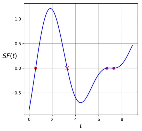
Figure 2. Switching function $SF\left(t\right)$ for $\epsilon =0.599$.

Lemma 2 is not satisfied in this case.

However, Lemma 2 will be fulfilled for $\epsilon =0.76$, as illustrated in Figure 3. Moreover, the optimal control law $u^{\ast }\left(t\right)$ defined by $SF\left(t\right)$ is shown.

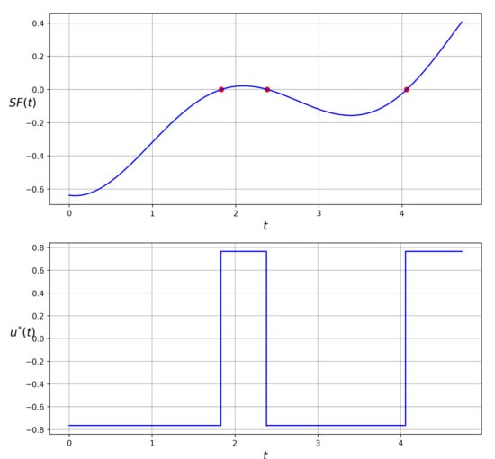
Figure 3. Switching function $SF\left(t\right)$ and optimal control $u^{\ast }\left(t\right)$ for $\epsilon =0.76$.

Vector C in this case: ${\displaystyle C=\left(\begin{array}{cccc}-0.14,& -0.72,& -0.48,& 0.46\end{array}\right).}$ The phase portraits of the first and second oscillators satisfy the given boundary conditions (44) and are presented in Figure 4.

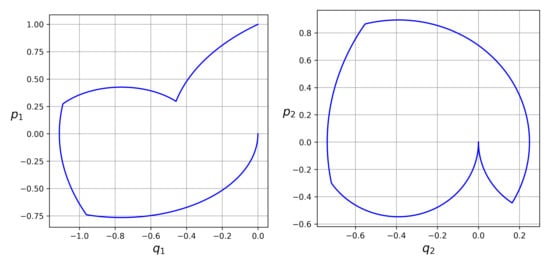
Figure 4. The phase portraits of the first and second oscillators.

The dependence of the criterion $T_0$ on the constraint $\epsilon$ is shown in Figure 5. The blue, red, and black curves show solutions for three-, four-, and five-switching control classes, which are defined by the boundaries of each control class. Figure 5 shows that $T_0\left(\epsilon \right)$ is a continuous function according to Lemma 6.

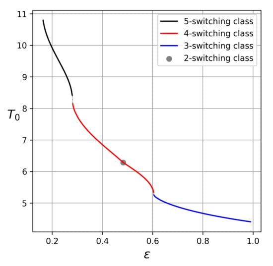
Figure 5. Dependence $T_0\left(\epsilon \right)$.

Figure 6 illustrates the dependencies of the control interval durations from $\epsilon$. The implicit function theorem shows that the durations of control intervals are continuous on $\epsilon$ inside each class, which can be observed in the graph. In area I, which corresponds to the five-switching class, the duration of the first control interval becomes zero when the boundary of the selected class $\left(\mathrm{I}\to \mathrm{II}\right)$ is reached. Region II corresponds to the four-switching class, where the second interval of I becomes the first interval, and it also becomes zero when it reaches the boundary $\left(\mathrm{II}\to \mathrm{III}\right)$. The third interval from region I becomes the second interval in II and the first interval in the three-switching region (III). If one of the internal intervals of the four-switching class is nullified, then the transition to the two-switching class takes place.

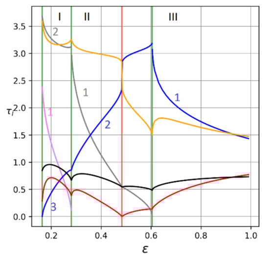
Figure 6. Dependencies ${\tau }_i\left(\epsilon \right)$.

Figure 7 shows the dependencies of the Jacobian for different switching control classes on $\epsilon$.

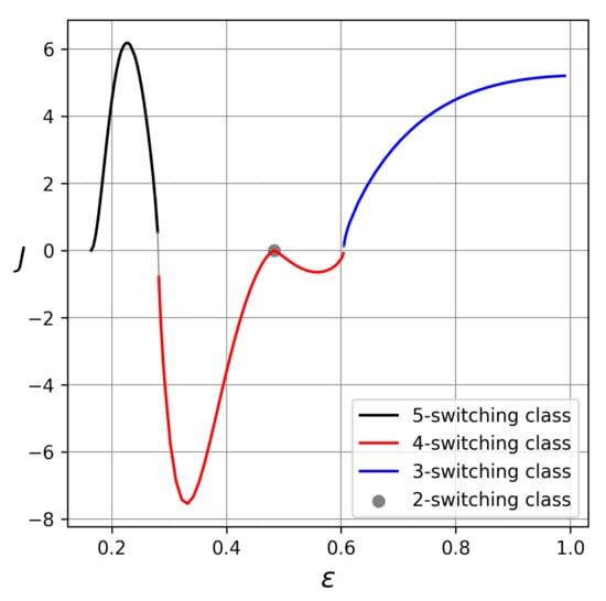
Figure 7. Dependence $J\left(\epsilon \right)$.

As one can see from the graph, when the class boundaries are reached, the Jacobians become equal to zero. Moreover, the Jacobian $J_4$ of the four-switching class is zero when passing to the two-switching class at one point. Lemma 1 is valid for the two-switching control class. Two-, three-, and four-switching control classes for different finite states of the first oscillator ($q_1^{T_0},p_1^{T_0}$) and $\epsilon =0.4$ are presented next. As before, it was checked that the obtained solutions for each final state form, according to Remark 3, the control law with the appropriate number of switchings.

6.2. The Phase Plane of the First Oscillator for Different Control Classes

Different control classes are shown in Figure 8. The red and green areas correspond to the three- and four-switching control classes with initial controls $-\epsilon ,\epsilon$, respectively. The reflections of these regions relative to the origins lead to blue and orange regions for the three- and four-switching control classes on the initial intervals $\epsilon ,-\epsilon$, respectively. The three-switching control classes are separated from each other by parametric curves obtained by Lemma 1. This is due to the fact that nullifying the lateral control interval in the three-switching control class also leads to the two-switching control class (orange and red curves). Zeroing the internal control interval in the ’four-switchings’ results in curves (blue and green) corresponding to the two-switching control classes at different initial controls. The yellow and gray boundary curves were obtained by moving from the four-switching class to the three-switching class by zeroing out the last control interval, with the control at the initial interval coinciding with the initial controls in the regions on either side of the boundary. The white and purple curves correspond to the zeroing of the first control interval in the four-switching class, which means the transition to the three-switching. The simultaneous nullifying of the side interval of the control constancy in the four-switching class corresponds to the blue points where the curves obtained under the conditions ${\tau }_1=0$ or ${\tau }_2=0$ intersect.

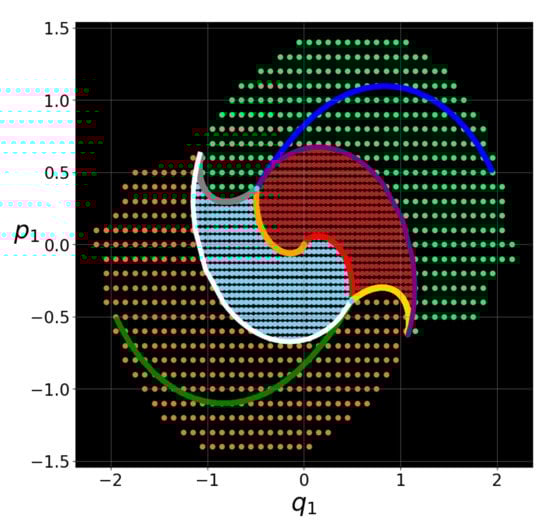
Figure 8. Terminal points of the phase plane of the first oscillator.

Figure 9 shows the dependence $T_0(p_1^{T_0},q_1^{T_0})$ of the criterion on the phase coordinates of the first oscillator. Three- and four-switching control classes are highlighted with red and green points. The colors of all curves correspond to the description in Figure 8.

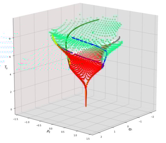
Figure 9. The dependence of the criterion $T_0$ on the phase coordinates of the first oscillator $(p_1^{T_0},q_1^{T_0})$.

7. Conclusions

Necessary and sufficient extremum conditions are proposed for the time-optimal control problem of a system consisting of two non-synchronous oscillators, and controlled by limited scalar impact. In addition, lemmas and theorems on the continuity of the criterion by the parameter are proposed. These results can be further extended to systems of any number of oscillators. Thus, a unified mathematical apparatus for describing the set of reachability of the first oscillator for systems of many oscillators will be developed in future works. The construction of control switching curves of the first oscillator in the phase plane will allow us to develop an approach to solving the problem of the synthesis of time-optimal control for multiple oscillators.

References

- Mirzaei, A.; Darabi, H. Mutual pulling between two oscillators. IEEE J. Solid-State Circuits 2014, 49, 360–372. [Google Scholar] [CrossRef]
- Salobutina, E. Regimes of more and more frequent switchings in the optimal control problem of oscillations of n oscillators. J. Math. Sci. 2008, 151, 3603–3610. [Google Scholar] [CrossRef]
- Kayumov, O. Time-optimal movement of platform with oscillators. Mech. Solids 2021, 56, 1622–1637. [Google Scholar] [CrossRef]
- Ansel, Q.; Chepelianskii, A.D.; Lages, J. Enhancing quantum exchanges between two oscillators. arXiv 2022, arXiv:2207.11156v1. [Google Scholar]
- Zhao, Y.; Chen, G.H. Two oscillators in a dissipative bath. Phys. A Stat. Mech. Appl. 2003, 317, 13–40. [Google Scholar] [CrossRef]
- Li, J.; Chen, Y.; Zhao, S. Periodic solutions and stability analysis for two-coupled-oscillator structure in optics of chiral molecules. Mathematics 2022, 10, 1908. [Google Scholar] [CrossRef]
- Firippi, E.; Chaves, M. Period-control in a coupled system of two genetic oscillators for synthetic biology. IFAC-PapersOnLine 2019, 52, 70–75. [Google Scholar] [CrossRef]
- Galyaev, A.A. Scalar control of a group of free-running oscillators. Autom. Remote Control 2016, 77, 1511–1523. [Google Scholar] [CrossRef]
- Galyaev, A.A. Impact of a system of material points against an absolutely rigid obstacle: A model for its impulsive action. Autom. Remote Control 2006, 67, 856–867. [Google Scholar] [CrossRef]
- Andresen, B.; Salamon, P.; Hoffmann, K.H.; Tsirlin, A.M. Optimal processes for controllable oscillators. Autom. Remote Control 2018, 79, 2103–2113. [Google Scholar] [CrossRef]
- Fedorov, A.; Ovseevich, A. Asymptotic control theory for a system of linear oscillators. Mosc. Math. J. 2016, 16, 561–598. [Google Scholar] [CrossRef]
- Pesch, H.J.; Plail, M. The Maximum Principle of optimal control: A history of ingenious ideas and missed opportunities. Control Cybern. 2009, 38, 973–995. [Google Scholar]
- Boltyansky, V.G. Mathematical Methods of Optimal Control, 2nd ed.; Nauka: Moscow, Russia, 1969. [Google Scholar]
- Chernousko, F.L.; Akulenko, L.D.; Sokolov, B.N. Oscillation Control; Nauka: Moscow, Russia, 1980. [Google Scholar]
- Berlin, L.M.; Galyaev, A.A. Extremum conditions for constrained scalar control of two nonsynchronous oscillators in the time-optimal control problem. Dokl. Math. 2022, 106, 286–290. [Google Scholar] [CrossRef]
- Sachkov, Y.L. Introduction to Geometric Control. arXiv 2021, arXiv:1903.00211v2. [Google Scholar]
- La Salle, J.P. The Time Optimal Control Problem. In Contributions to the Theory of Nonlinear Oscillations; Princeton University Press: Princeton, NJ, USA, 1960; Volume 5, pp. 1–24. [Google Scholar]
- Berlin, L.M.; Galyaev, A.A.; Lysenko, P.V. About time-optimal control problem for system of two non-synchronous oscillators. In Proceedings of the 16th International Conference on Stability and Oscillations of Nonlinear Control Systems (Pyatnitskiy’s Conference), Moscow, Russian, 1–3 June 2022. [Google Scholar] [CrossRef]
- Zorich, V.A. Mathematical Analysis I, 2nd ed.; Springer: Berlin/Heidelberg, Germany, 2015; p. 616. [Google Scholar]
- Isaacs, R. Differential Games: A Mathematical Theory with Applications to Warfare and Pursuit, Control and Optimization; John Wiley and Sons: New York, NY, USA, 1965. [Google Scholar]
Publisher’s Note: MDPI stays neutral with regard to jurisdictional claims in published maps and institutional affiliations. |
© 2022 by the authors. Licensee MDPI, Basel, Switzerland. This article is an open access article distributed under the terms and conditions of the Creative Commons Attribution (CC BY) license (https://creativecommons.org/licenses/by/4.0/).