From Multi- to Univariate: A Product Random Variable with an Application to Electricity Market Transactions: Pareto and Student’s t-Distribution Case

Abstract

Multivariate modelling of economics data is crucial for risk and profit analyses in companies. However, for the final conclusions, a whole set of variables is usually transformed into a single variable describing a total profit/balance of company’s cash flows. One of the possible transformations is based on the product of market variables. Thus, in this paper, we study the distribution of products of Pareto or Student’s t random variables that are ubiquitous in various risk factors analysis. We review known formulas for the probability density functions and derive their explicit forms for the products of Pareto and Gaussian or log-normal random variables. We also study how the Pareto or Student’s t random variable influences the asymptotic tail behaviour of the distribution of their product with the Gaussian or log-normal random variables and discuss how the dependency between the marginal random variables of the same type influences the probabilistic properties of the final product. The theoretical results are then applied for an analysis of the distribution of transaction values, being a product of prices and volumes, from a continuous trade on the German intraday electricity market.

1. Introduction

A comprehensive approach to risk management should involve multivariate modelling of economics data as interactions between market variables cannot be simply neglected. However, for the final conclusions a whole set of variables is usually transformed into a single variable describing a total profit/balance of company’s cash flows. Often, this transformation is based on the product of market variables. Among many others, these are, e.g., quotes of commodities in the operational currency of a company, being the product of prices and exchange rates [1], economic variables with random discount factors [2], and company’s profit with random tax rates [3] or transaction values, being the product of prices and volumes. The latter case will be further illustrated in Section 6 based on the German continuous electricity market data.

In this paper, we analyze the probabilistic properties of the product random variable defined as

$$Z=XY,$$

(1)

where X and Y, called marginal random variables, have continuous distributions. In a general case, the probability density function (PDF) of Z is given by [4,5]

$$f_Z\left(z\right)={\int }_{-\infty }^{\infty }\frac{1}{\mid x\mid }{f}_{X,Y}\left(x,\frac{z}{x}\right)dx,$$

(2)

where $f_{X,Y}(x,y)$, $x,y\in \mathbb{R}$ is a two-dimensional PDF of the vector $(X,Y)$. Obviously, the general properties of the product simplify when the marginal random variables are independent. In that case, the corresponding bi-dimensional random vector has the PDF that is a product of the marginal densities, i.e., we have

$$f_Z\left(z\right)={\int }_{-\infty }^{\infty }\frac{1}{\mid x\mid }{f}_X\left(x\right)f_Y\left(\frac{z}{x}\right)dx,$$

(3)

where $f_X\left(x\right)$ and $f_Y\left(y\right)$ are the PDF’s of the marginal distributions corresponding to X and Y, respectively.

In this paper, we separately study the cases when at least one random variable is Pareto [6] or Student’s t distributed [7]. These distributions belong to the so-called heavy-tailed class of distributions, for which the variance may be infinite. Therefore, they are appropriate for modelling phenomena with a high probability of extreme observations. On the other hand, for both distributions, the probability density function is given by an explicit formula, being convenient for statistical analyses. As a consequence, the Pareto and Student’s t distributions are frequently used in various interesting applications; see, e.g., [8,9,10,11]. Both considered heavy-tailed distributions are also crucial in risk analysis and were applied for description of variables describing the risk factors from different areas of interest. See, e.g., Refs. [12,13,14,15] for an application of the Student’s t distribution and Refs. [16,17,18,19]—for the Pareto distribution. The Pareto distribution is skewed with power-law tails, while the Student’s t distribution is symmetric and bell-shaped. It resembles the normal distribution for large values of the degrees of freedom parameter.

We start with an analysis of the joint Pareto (or Student’s t) distribution of the marginal variables. In this case, we examine how dependency between the variables (expressed by means of the correlation coefficient for the finite-variance case) influences the probabilistic properties of the final product. Next, we consider the case, when the marginal random variables belong to different classes, i.e., heavy-tailed and finite-variance distributions. The first class is represented here by the Pareto or Student’s t distributions while the second-one by the Gaussian or log-normal ones. In each case, we give the formula for the product PDF. In particular, explicit forms are derived for the products of Pareto and Gaussian or log-normal distributions and, for completeness, recalled from the literature for the product of two independent Pareto variables with different shape parameters [3] and the product of Student’s t and Gaussian variables [7]. The asymptotic behaviour of the PDF is shown for all products with independent Pareto random variable and for the product of the Gaussian and Student’s t variables. We also calculate the expected value and the variance (if they exist) for all independent cases.

The theory related to the product random variables has found many interesting applications; see Section 2. Here, the methodology is applied to real data from the energy market. We analyze the distribution of the transaction values, being a product of prices and volumes, from a continuous trade on the German intraday electricity market. We show that, using the derived product distribution, a fit to the transaction values data can be obtained, being at the same time consistent with the corresponding prices and volumes distributions.

The first main contribution of the paper is the analysis how the dependence between marginal random variables coming from given joint distribution (here Pareto or Student’s t) influences the properties of their product. According to our knowledge, such analyses are rarely discussed in the literature; however, they may be crucial in real applications. The second contribution is the analysis of the product random variables coming from different classes of distributions and investigation of how the parameter responsible for the heavy-tailed behavior of one of the variables influences the asymptotic tail of the final product. Finally, we propose the estimation procedure for the product random variable and demonstrate its efficiency for simulated data.

The rest of the paper is organized as follows: In Section 2, we present the previous studies related to product random variables and indicate our contribution to this theory. In Section 3, we conduct a theoretical study on the product distribution in the case, when at least one variable has the Pareto distribution. The analogous analysis for the Student’s t distribution is derived in Section 4. Next, in Section 5, the obtained theoretical properties are used for the simulation study on the estimation of the parameters of the product distribution. A possible application of the obtained results is illustrated in Section 6, while Section 7 concludes the paper. Potential future research directions are then discussed in Section 8. Additionally, for completeness, in the Appendix A we give the main properties of the product of the considered representatives of the finite-variance class of distributions, i.e., the Gaussian and log-normal one.

2. State of the Art

In the literature, there are various examples of random variables for which the product is analyzed in theory and practice. Particular emphasis is placed on the product of two random variables that come from the same class of distributions; see, e.g., [20,21,22,23,24]. A special attention is paid to the case when two considered random variables are Gaussian or Student’s t distributed; see, e.g., [4,7,25,26,27,28]. The other interesting cases one can find also in [29], where exponentially distributed random variables are considered or in [30], where Dirichlet distributed random variables are examined. For other references, see also [31,32,33,34].

Many authors analyze also the products of random variables having similar probabilistic properties. We mention here the interesting research related to non-negative random variables [35], continuous random variables [36], symmetric random variables [37], subexponential random variables [38] or regular-variation-tailed random variables [39]. See also [40].

Different classes of distributions are also considered in the literature and the product of such random variables is analyzed; see, e.g., [34,41,42,43,44,45,46] and references therein. General properties of the products of subexponential and long-tailed class were studied by [47]. A particular attention was also paid on the studies of the product of Pareto and Kumaraswamy random variables [48], Pearson (type VII) and Laplace random variables [49], Pareto and Rayleigh random variables [50] or product of Beta, Gamma and Gaussian random variables [51]. Our studies presented in this paper are related to both cases, i.e., when random variables come from the same as well as different classes of distributions.

Most of the theoretical studies are dedicated to the cases when the considered random variables are independent; see, e.g., [52,53,54]; however, there are also articles where a product of two correlated random variables is examined; see, e.g., [2,55,56]. In this paper, we consider both cases, namely when the random variables are independent as well as correlated.

When one considers product random variables, the main attention is paid on their moments [28,35,57], probability distribution (i.e., PDF) [51,54,55] or other statistical characteristics [24,52]. However, there are also analyses related to tails behavior [2,38,39,47,58] or other asymptotic properties [40,53,59]. In this paper, we also study the basic characteristics of product random variables, like the PDF and moments, but we also examine their tail behavior.

We also refer the readers to the general theory of a random variables arising as a product [57,60] or studies devoted to representations of some random variables expressed as a product [61].

Beyond theoretical considerations, the random variables that arise as a product (or other functions) of two variables have found various interesting applications including finance, economy, but also physical sciences, reliability theory, hydrology, and many others; see, e.g., [1,45,62,63,64,65,66,67] and the corresponding comments in [2,68,69,70]. The theory of product random variables was applied also in cognitive radio networks [40], sociological models [70], risk theory [2] or wireless communication systems [24]. In this paper, the proposed methodology is applied to the transaction values from the energy market.

3. Pareto Distribution

In this section, we study probabilistic properties of the product of two random variables in the case when at least one of them is Pareto distributed. The second variable is either dependent Pareto distributed, independent Pareto distributed or belonging to the finite-variance class, represented by the Gaussian or log-normal distribution.

3.1. Product of Two Pareto Distributed Random Variables

The two-dimensional Pareto distributed random vector $(X,Y)$ with parameters $a,{\theta }_X,$${\theta }_Y>0$ has the following PDF [6]:

$$f_{X,Y}(x,y)=\frac{a(a+1){\left({\theta }_X{\theta }_Y\right)}^{a+1}}{{(x{\theta }_Y+y{\theta }_X-{\theta }_X{\theta }_Y)}^{a+2}},x>{\theta }_X,y>{\theta }_Y.$$

(4)

The above parametrization corresponds to the Pareto distribution of the first kind [71]. The shape parameter a is responsible for the behavior of the distribution tail. The marginal distributions of X and Y are given by

$$\begin{array}{c}\hfill f_X\left(x\right)=\frac{a{\theta }_X^a}{x^{a+1}},x>{\theta }_X,f_Y\left(y\right)=\frac{a{\theta }_Y^a}{y^{a+1}},y>{\theta }_Y.\end{array}$$

(5)

Note that the parameter a is the same for both marginal distributions. For $a>2$, the random variables X and Y described by the PDF (4) are positively correlated. The covariance and correlation are given by, respectively,

$$\begin{array}{c}\hfill \mathrm{cov}(X,Y)=\frac{{\theta }_X{\theta }_Y}{{(a-1)}^2{(a-2)}^2},\mathrm{corr}(X,Y)=\frac{1}{a}.\end{array}$$

(6)

It is interesting to note that, here, the correlation between the marginal variables is governed by the shape parameter a. As a consequence, with such parametrization, X and Y are always positively correlated.

When the random vector $(X,Y)$ is described by the PDF given in Equation (4), using Formula (2), one obtains

$$f_Z\left(z\right)=(a+1)a{\left({\theta }_X{\theta }_Y\right)}^{a+1}\underset{{\theta }_X}{\overset{\frac{z}{{\theta }_Y}}{\int }}\frac{1}{x}{({\theta }_{Y}x+{\theta }_X\frac{z}{x}-{\theta }_X{\theta }_Y)}^{-a-2}dx,z>{\theta }_X{\theta }_Y,$$

(7)

where $f_Z(·)$ is the PDF of the product of X and Y. The integral in Equation (7) has no closed form and can be expressed by means of the Appel hypergeometric special function. However, one can obtain its value with numerical calculations.

As one can see, the two-dimensional Pareto distribution defined by the PDF in Equation (4) does not cover the case with uncorrelated marginal random variables. In the case when X and Y are independent and are described by the Pareto distributions of the PDFs given in (5) with $a_X,{\theta }_X>0$ and $a_Y,{\theta }_Y>0$, respectively, then the PDF of the vector $(X,Y)$ is given by the product of the marginal PDFs, $f_X\left(x\right)$ and $f_Y\left(y\right)$ and the PDF of the product Z, given in Equation (1), can be explicitly derived.

Lemma 1.

Assume that independent random variables X and Y have the Pareto distribution with parameters $a_X,{\theta }_X$ and $a_Y,{\theta }_Y$, respectively. Then, for $a_X\ne a_Y$, the random variable Z defined in (1) has the following PDF:

$$f_Z\left(z\right)=a_X{a}_Y\left(\frac{z^{-a_X-1}{\left({\theta }_X{\theta }_Y\right)}^{a_X}}{a_Y-a_X}+\frac{z^{-a_Y-1}{\left({\theta }_X{\theta }_Y\right)}^{a_Y}}{a_X-a_Y}\right),z>{\theta }_X{\theta }_Y.$$

(8)

When $a_X=a_Y=a$, then the PDF of Z has the following form:

$$\begin{array}{c}\hfill f_Z\left(z\right)=a^2\left({\theta }_X{\theta }_Y\right)z^{-a-1}log\left(\frac{z}{{\theta }_X{\theta }_Y}\right),z>{\theta }_X{\theta }_Y.\end{array}$$

(9)

Proof. 

The proof comes directly from formula (3) and the fact that the PDF of the random vector $(X,Y)$ is given by the product of marginal PDFs of X and Y for $a_X\ne a_Y$ and $a_X=a_Y=a$. Note that the PDF formula for $a_X\ne a_Y$ is a special case of the PDF of the product of n independent Pareto random variables, derived in [3]. □

When one considers a random vector of the two-dimensional Pareto distribution defined by the PDF in Equation (4), then there are no closed forms for the expectation (when $a>1$) and the variance (when $a>2$) of the random variable Z. However, when X and Y are independent random variables, then the expected value and the variance of the random variable Z are given by [6]

$$\begin{array}{cc}\hfill \mathbb{E}\left(Z\right)& =\frac{{\theta }_X{\theta }_Y{a}_X{a}_Y}{(a_X-1)(a_Y-1)},a_X,a_Y>1,\hfill \end{array}$$

(10)

$$\begin{array}{cc}\hfill \mathbb{V}\mathrm{ar}\left(Z\right)& ={\theta }_X^2{\theta }_Y^2{a}_X{a}_Y\left[\frac{{(a_X-1)}^2+{(a_Y-1)}^2-1}{(a_X-2)(a_Y-2){(a_X-1)}^2{(a_Y-1)}^2}\right],a_X,a_Y>2.\hfill \end{array}$$

(11)

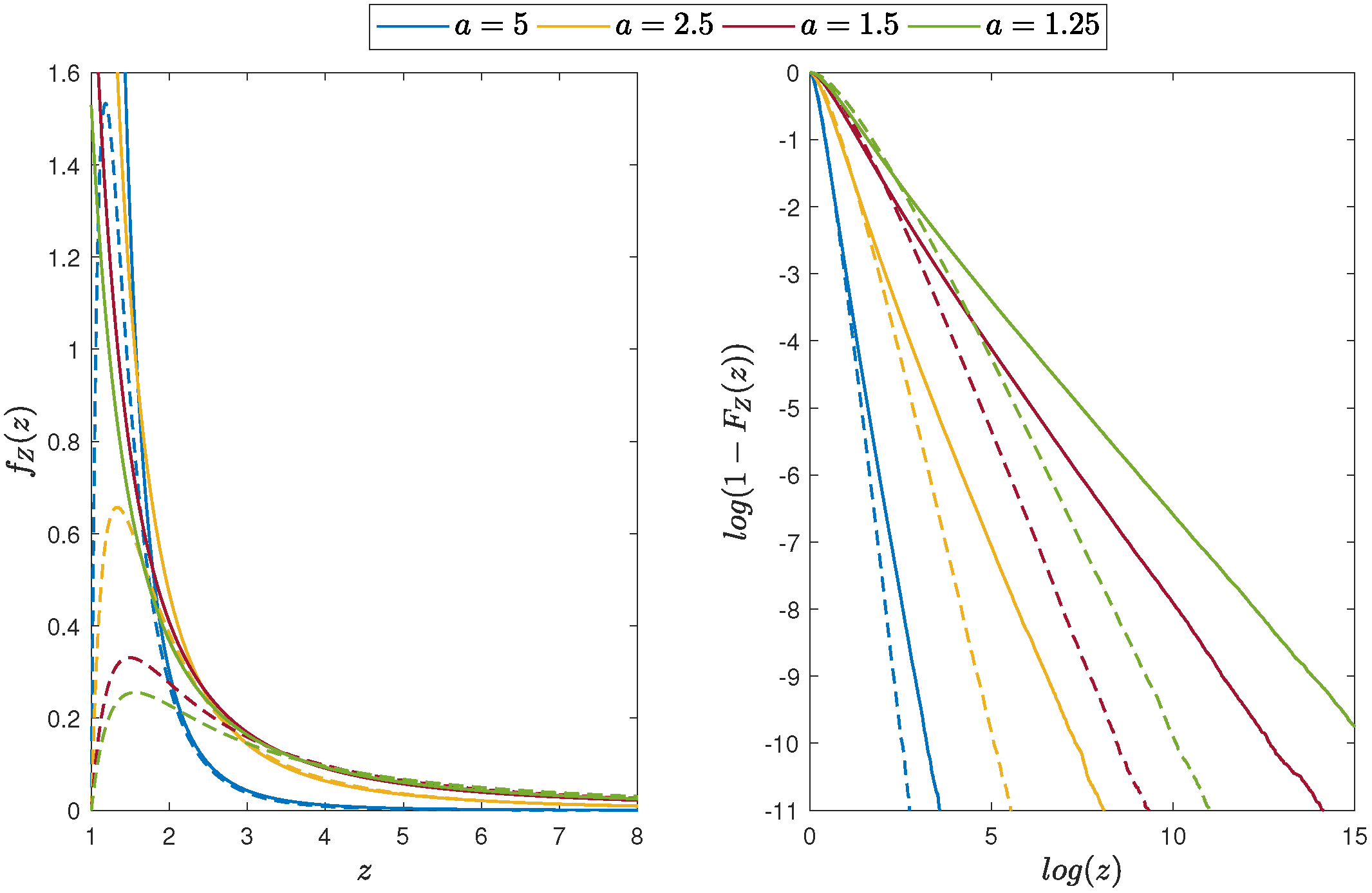
In Figure 1, we plot the PDF and the corresponding distribution tail of the random variable Z that is a product of marginal random variables from the two-dimensional Pareto distribution described by the PDF (4) for different values of the a parameter. Recall that the correlation (if exists) is directly related to the shape parameter a; see (6). Thus, it is influenced by the distribution tails. With larger a (lower $\mathrm{corr}(X,Y)$), the probability of extreme observations becomes lower. In all cases, the distribution tails behave like a power function with a clear linear shape in the double logarithmic scale. For comparison, we also show the plots for the corresponding product of independent Pareto marginal variables. In this case, the probabilities of extreme observations are lower than for the corresponding dependent Pareto distribution, but the power tail behavior is preserved.

Figure 1. Distribution of the product of marginal random variables from the two-dimensional Pareto distribution with ${\theta }_X={\theta }_Y=1$ and different values of the a parameter. (Left panel): the PDF of the random variable Z. (Right panel): the distribution tail for the random variable Z (in log-log scale). The dotted lines correspond to the case when X and Y are independent and $a_X=a_Y=a$, ${\theta }_X={\theta }_Y=1$. The colors of the solid and dotted lines correspond to the same a parameter.

3.2. Product of Gaussian and Pareto Distributed Random Variables

In this section, we assume that X is a Gaussian random variable with parameters ${\mu }_X=0$ and ${\sigma }_X>0$ and Y is a Pareto distributed random variable with parameters $a_Y>0$ and ${\theta }_Y>0$ defined in the previous subsection. Moreover, we assume that X and Y are independent. Note that the main probabilistic properties of the two-dimensional Gaussian distribution and its product are recalled in the Appendix A for completeness.

Lemma 2.

The random variable Z defined as a product of X and Y has the following PDF:

$$\begin{array}{c}\hfill f_Z\left(z\right)=\frac{a_Y{\theta }_Y^{a_Y}{\sigma }_X^{a_Y}}{\sqrt{2\pi }\mid z {\mid }^{a_Y+1}}{2}^{(a_Y-1)/2}\gamma \left(\frac{a_Y+1}{2},\frac{z^2}{2{\sigma }^2{\theta }_Y^2}\right),z\in \mathbb{R},\end{array}$$

(12)

where $\mathsf{\Gamma }(·)$ is the Gamma function, i.e., $\mathsf{\Gamma }\left(\alpha \right)={\int }_0^{\infty }{t}^{\alpha -1}{e}^{-t}dt$, and $\gamma (·,·)$ is the upper incomplete Gamma function defined as $\gamma (\alpha ,x)={\int }_0^x{t}^{\alpha -1}exp\{-t\}dt$.

The proof of this lemma is given in the Appendix B.

Using the fact that $\gamma (\alpha ,x)\to \mathsf{\Gamma }\left(\alpha \right)$ when $x\to \infty$, for $z\to \infty$, we have

$$\begin{array}{c}\hfill f_Z\left(z\right)\sim \frac{a_Y{\theta }_Y^{a_Y}{\sigma }_X^{a_Y}}{\sqrt{2\pi }\mid z {\mid }^{a_Y+1}}{2}^{(a_Y-1)/2}\mathsf{\Gamma }\left(\frac{a_y+1}{2}\right).\end{array}$$

(13)

This indicates that the PDF of Z has a power-law behavior and thus, in the considered case, the Pareto distribution dominates the tail behavior.

The expected value of Z in the considered case, when $a_Y>1$, is equal to zero, and the variance of Z, if $a_Y>2$, is given by

$$\mathbb{V}\mathrm{ar}\left(Z\right)=\frac{{\left({\theta }_Y{\sigma }_X\right)}^2{a}_Y}{(a_Y-2)}.$$

(14)

The variance decreases to the square of the product of the marginal variables scale parameters, ${\left({\theta }_Y{\sigma }_X\right)}^2$, as the Pareto shape parameter $a_Y\to \infty$.

In Figure 2, we plot the PDF and the corresponding distribution tail of the random variable Z that is a product of two independent random variables from the Gaussian and Pareto distributions for different values of the parameter $a_Y$. Moreover, in Figure 3, we demonstrate the comparison of the PDFs and distribution tails of X and Y, and the corresponding random variable Z for selected values of the parameters. One can see that the product has a lighter tail than the Pareto distributed random variable but a heavier tail than the Gaussian one. However, the power-law behavior, which corresponds to Equation (13), can be easily observed.

Figure 2. Distribution of the product of two independent random variables from the Gaussian and Pareto distribution with ${\mu }_X=0$ and ${\sigma }_X={\theta }_Y=1$ and different values of the $a_Y$ parameter. (Left panel): the PDF of the random variable Z. (Right panel): the distribution tail for the random variable Z (in log-log scale).

Figure 3. (Left panel): the PDF of the random variables X (Gaussian), Y (Pareto) and Z. (Right panel): the distribution tails. The parameters are: ${\mu }_X=0$, ${\sigma }_X={\theta }_Y=1$ and $a_Y=0.5$.

3.3. Product of Log-Normal and Pareto Distributed Random Variables

In this part, we assume that X is a log-normally distributed random variable with parameters ${\mu }_X=0$ and ${\sigma }_X>0$, and Y is a Pareto distributed random variable with parameters $a_Y>0$ and ${\theta }_Y>0$. Moreover, assume that X and Y are independent. Note that the main probabilistic properties of the two-dimensional log-normal distribution and its product are given in the Appendix B for completeness.

Lemma 3.

The random variable Z defined as a product of X and Y has the following PDF:

$$\begin{array}{ccc}\hfill f_Z\left(z\right)& =& \frac{a_Y{\theta }_Y^{a_Y}exp\left\{\frac{a_Y^2{\sigma }_X^2}{2}\right\}}{z^{a_Y+1}}\mathsf{\Phi }\left(\frac{log(z/{\theta }_Y)-a_Y{\sigma }_X^2}{{\sigma }_X}\right),z>0,\hfill \end{array}$$

where $\varphi (·)$ and $\mathsf{\Phi }(·)$ are the PDF and cumulative distribution function (CDF) of the standard Gaussian distribution, respectively.

The proof of this lemma is presented in the Appendix B. Note that, since the function $\mathsf{\Phi }(·)$ is monotonically converging to 1 as $z\to \infty$, the tail behaviour of the product random variable Z is dominated by the power function, governed by the Pareto shape parameter $a_Y$.

The expected value of Z (when $a_Y>1$) and the variance of Z (when $a_Y>2$) are given by

$$\mathbb{E}\left(Z\right)=\frac{{\theta }_Y{a}_Y}{a_Y-1}exp\left\{\frac{{\sigma }_X^2}{2}\right\},$$

(15)

$$\mathbb{V}\mathrm{ar}\left(Z\right)=\frac{{\theta }_Y^2{a}_{Y}exp\left\{2{\sigma }_X^2\right\}}{{(a_Y-1)}^2}\left(\frac{1}{a_Y-2}+a_Y-a_{Y}exp\{-{\sigma }_X^2\}\right).$$

(16)

Here, both marginal variables can take only positive values. Hence, the product variable Z is also positive and its expected value (if it exists) is greater than 0, $\mathbb{E}\left(Z\right)>0$. The expected value as well as the variance of Z are the products of the corresponding moments of the marginal distributions. Their existence is directly related to the existence of the moments of the Pareto marginal distribution.

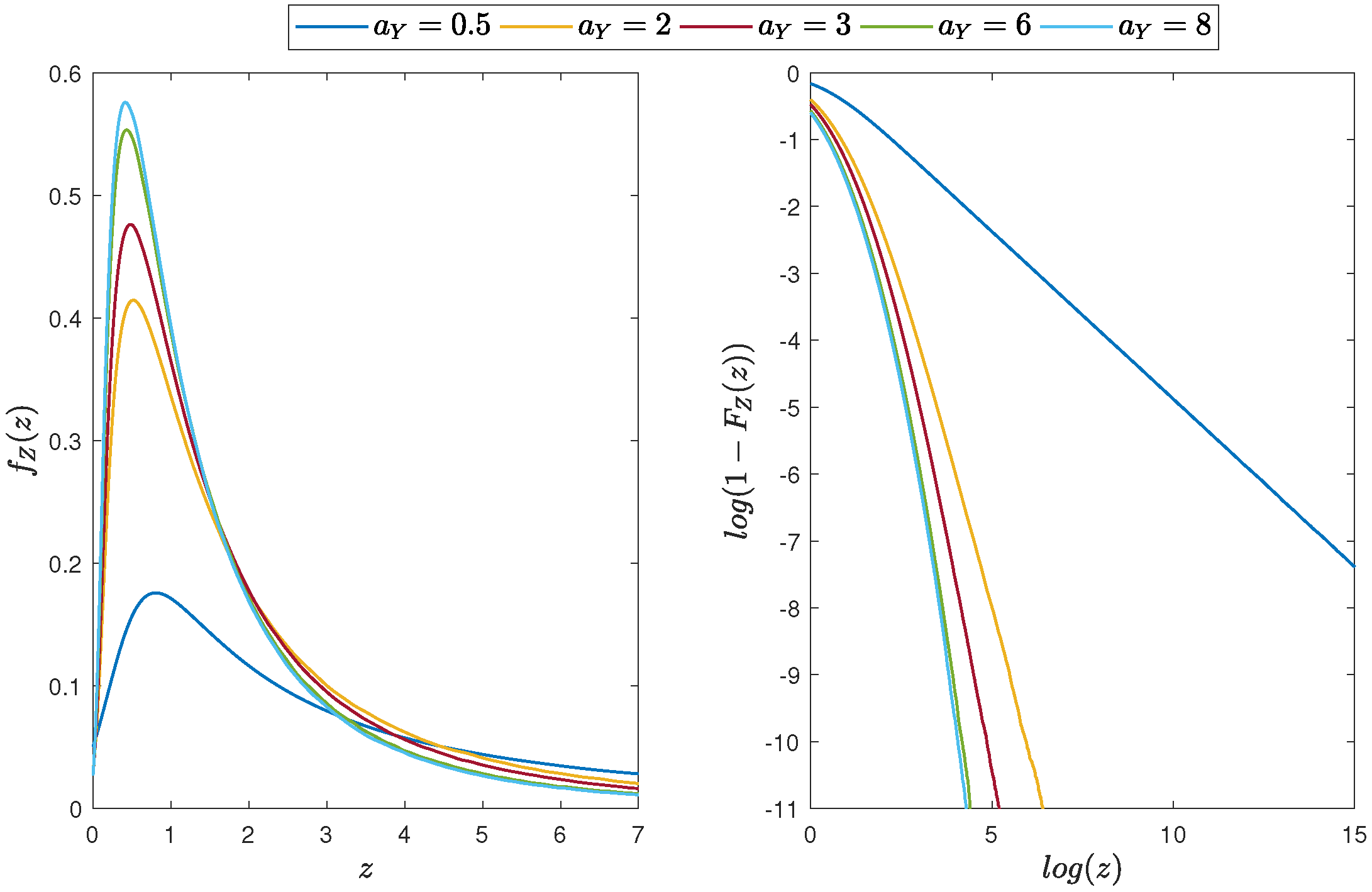
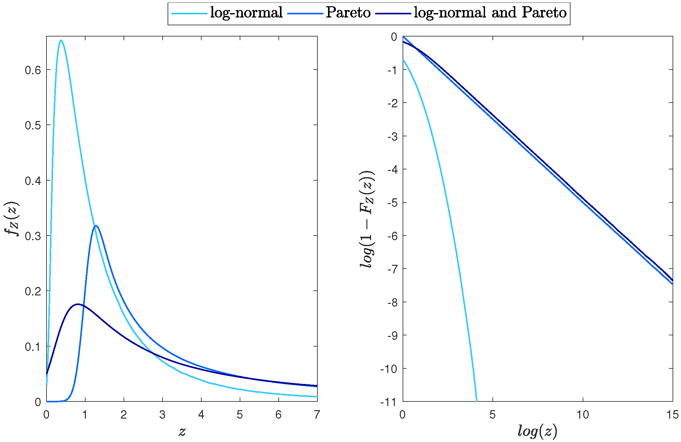
In Figure 4, we plot the PDF of the random variable Z and the corresponding distribution tail for different values of the parameter $a_Y$, while, in Figure 5, we demonstrate the comparison of the X, Y and Z distributions. As can be observed, the tail parameter of the marginal Pareto distribution has a large impact on the tail of the product distribution. Differently than for the Gaussian distribution, the probability of extreme observations is greater for the product than for both individual random variables.

Figure 4. Distribution of the product of two independent random variables from the log-normal and Pareto distribution with ${\mu }_X=0$ and ${\sigma }_X={\theta }_Y=1$ and different values of $a_Y$ parameter. (Left panel): the PDF of the random variable Z. (Right panel): the distribution tail for the random variable Z (in log-log scale).

Figure 5. (Left panel): the PDF of the random variables X (log-normal), Y (Pareto) and Z. (Right panel): the distribution tails. The parameters are equal: ${\mu }_X=0$ and ${\sigma }_X={\theta }_Y=1$ and $a_Y=0.5$.

4. Student’s t Distribution

In this section, we consider another representative of the class of heavy-tailed distributions, namely the Student’s t. Similarly as for the Pareto case, we examine how the dependence of two Student’s t distributed random variables influences their product’s distribution. We also consider the product of Student’s t and Gaussian as well as Student’s t and log-normally distributed random variables and indicate how the heavy-tailed behavior of the Student’s t distribution influences the distribution of the final product.

4.1. Product of Two Student’s t Distributed Random Variables

A common method of constructing a two-dimensional Student’s t distributed random vector $(X,Y)$ is based on the following observation. Let us assume that $(N_1,N_2)$ is a two-dimensional Gaussian vector defined by the PDF in Equation (A1) with the parameters ${\mu }_X={\mu }_Y=0$, ${\sigma }_X={\sigma }_Y=1$ and $\rho \in (-1,1)$, and ${\chi }^2$ is a one-dimensional random variable with chi-square distribution with $n>0$ degrees of freedom. Moreover, assume that $(N_1,N_2)$ and ${\chi }^2$ are independent. Then, the random vector defined as

$$\begin{array}{c}\hfill (X,Y)=\sqrt{n/{\chi }^2}(N_1,N_2)\end{array}$$

(17)

has the two-dimensional Student’s t distribution with n degrees of freedom, and its PDF is given by [72]

$$f_{X,Y}(x,y)=\frac{1}{2\pi \sqrt{1-{\rho }^2}}{\left[1+\frac{x^2-2\rho xy+y^2}{n(1-{\rho }^2)}\right]}^{-\frac{n+2}{2}},x,y\in \mathbb{R}.$$

(18)

The marginal random variable X (and Y) has the one-dimensional Student’s t distribution defined by the following PDF [73]:

$$\begin{array}{c}\hfill f_X\left(x\right)=\frac{\mathsf{\Gamma }\left(\right(n+1)/2)}{\sqrt{n\pi }\mathsf{\Gamma }(n/2)}{\left(1+\frac{x^2}{n}\right)}^{-(n+1)/2},x\in \mathbb{R},\end{array}$$

(19)

where $\mathsf{\Gamma }(·)$ is the gamma function. Note that the number of degrees of freedom, n, is equal for both marginal variables. For $n>2$, the random variables X and Y described by the PDF in (18) have the following covariance:

$$\begin{array}{c}\hfill \mathrm{cov}(X,Y)=\frac{n}{n-2}\rho .\end{array}$$

(20)

One can see that, although the zero correlation coefficient corresponds to $\mathrm{cov}(X,Y)=0$, it is not equivalent to the independence of the random variables X and Y, since in that case the PDF of a random vector $(X,Y)$ (see Equation (18)) is not a product of the PDFs of the marginal distributions (see Equation (19)). The cases $\rho =1$ and $\rho =-1$ are not analyzed in this paper. However, let us note that in this case the product of the random variables X and Y is a squared Student’s t distributed random variable multiplied by some constant value. Depending on the sign of $\rho$, the product random variable takes only positive or only negative values.

In the case when the random vector $(X,Y)$ is described by the PDF given in Equation (18), then, using Formula (2), one obtains

$$\begin{array}{c}\hfill f_Z\left(z\right)=\frac{1}{\pi \sqrt{1-{\rho }^2}}{\int }_0^{\infty }\frac{1}{x}{\left[1+\frac{x^2-2\rho z+\frac{z^2}{x^2}}{n(1-{\rho }^2)}\right]}^{-\frac{n+2}{2}}dx,x\in \mathbb{R}.\end{array}$$

(21)

The integral in Equation (21) has no closed form and can be expressed by means of the Appel hypergeometric special function. Obviously, one can obtain its value with numerical calculations.

If the random variables X and Y are independent and are described by the Student’s t distributions of PDFs given in Equation (19) with degrees of freedom $n_X>0$ and $n_Y>0$ corresponding to X and Y, respectively, then the PDF of the vector $(X,Y)$ is given by a product of marginal densities of X and Y. Thus, the product random variable Z has the following PDF for $z\in \mathbb{R}$ [7]

$$f_Z\left(z\right)=\frac{2\mathsf{\Gamma }\left(\frac{n_X+1}{2}\right)\mathsf{\Gamma }\left(\frac{n_Y+1}{2}\right)}{\sqrt{n_X{n}_Y}\pi \mathsf{\Gamma }\left(\frac{n_X}{2}\right)\mathsf{\Gamma }\left(\frac{n_Y}{2}\right)}{\int }_0^{\infty }\frac{1}{x}{\left(1+\frac{x^2}{n_X}\right)}^{-\frac{n_X+1}{2}}{\left(1+\frac{z^2}{x^2{n}_Y}\right)}^{-\frac{n_Y+1}{2}}dx.$$

(22)

Similarly as in the previous case, the above integral can be expressed using special functions; see [74].

It is interesting to note that the PDFs of the product, $f_Z(·)$, behave differently in the dependent with $\rho =0$ (see Equation (21)) and independent (see Equation (22)) case. Indeed, in the dependent case with $\rho =0$, we have

$$f_Z\left(z\right)=\frac{1}{\pi }{\int }_0^{\infty }\frac{1}{x}{\left[1+\frac{x^2+\frac{z^2}{x^2}}{n}\right]}^{-\frac{n+2}{2}}dx,x\in \mathbb{R},$$

(23)

while in the independent case with $n_X=n_Y=n$, the product’s PDF is given by

$$f_Z\left(z\right)=\frac{2\mathsf{\Gamma }{\left(\frac{n+1}{2}\right)}^2}{n\pi \mathsf{\Gamma }{\left(\frac{n}{2}\right)}^2}{\int }_0^{\infty }\frac{1}{x}{\left(1+\frac{x^2+\frac{z^2}{x^2}}{n}+\frac{z^2}{n^2}\right)}^{-\frac{n+1}{2}}dx.$$

(24)

When one considers the random vector of the two-dimensional Student’s t distribution defined by the PDF in Equation (18), then the expectation (when $n>1$) and the variance (when $n>2$) of the random variable Z can be calculated based on its PDF (see Equation (21)). In this case, there are no closed forms for the mentioned statistics. However, when X and Y are independent random variables, then the expected value (if $n_X,n_Y>1$) and the variance (if $n_X,n_Y>2$) of the random variable Z are given by [7]

$$\begin{array}{c}\hfill \mathbb{E}\left(Z\right)=0,\mathbb{V}ar\left(Z\right)=\frac{n_X{n}_Y}{(n_X-2)(n_Y-2)}.\end{array}$$

(25)

The variance of the product of independent marginal variables is just a product of the individual variances. Moreover, it tends to the variance of one of the variables if the number of degrees of freedom of the second variable, $n_X$ or $n_Y$, goes to infinity. If both parameters, $n_X,n_Y\to \infty$, then the variance of the product decreases to 1.

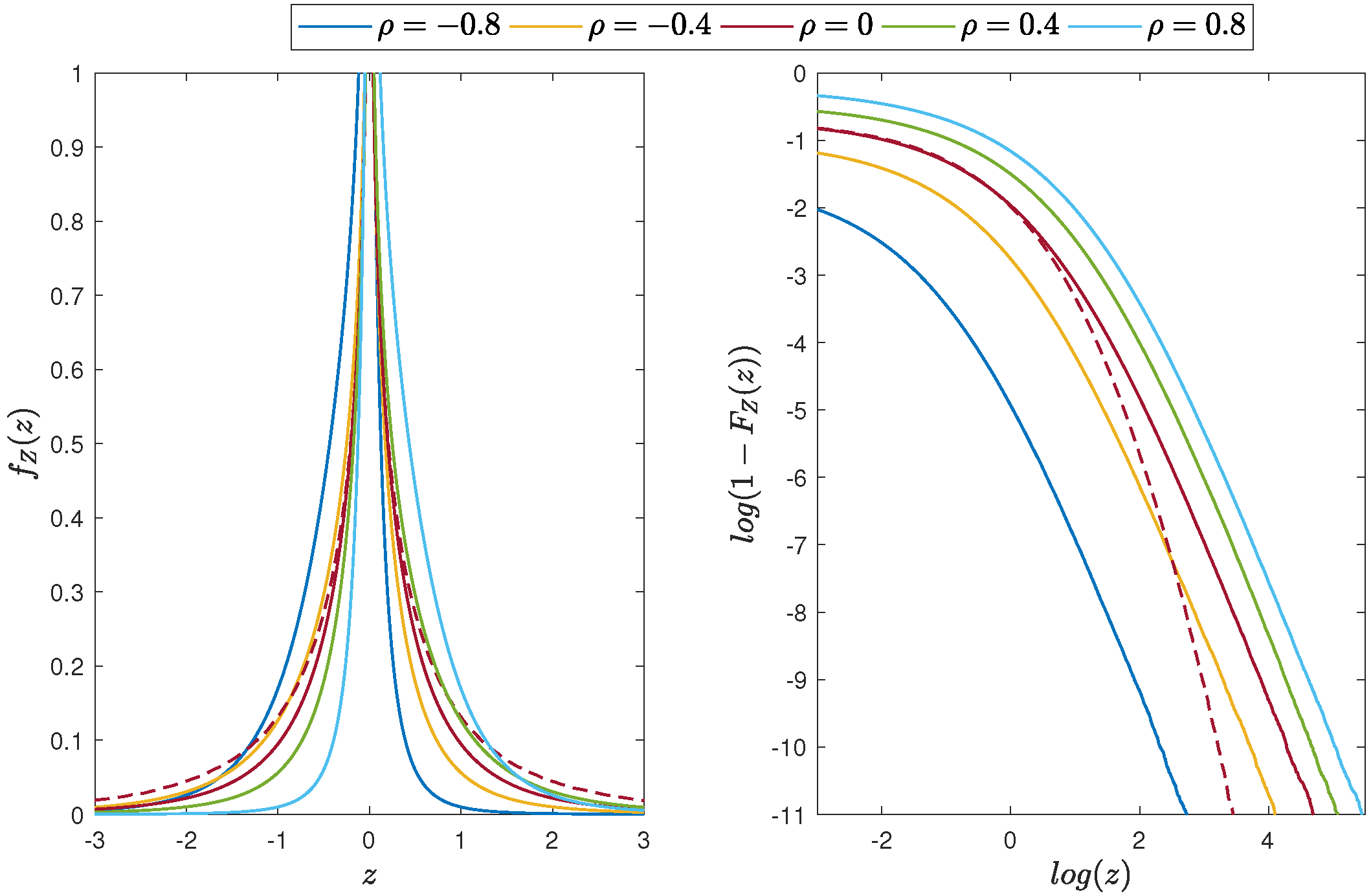
In Figure 6, we demonstrate the PDF and the distribution tails of the random variable Z that is a product of marginal random variables from the two-dimensional Student’s t distribution described by the PDF (18) for different values of the parameter $\rho$. The resulting PDF is symmetric only if $\rho =0$. Otherwise, it is right-skewed for $\rho >0$ and left-skewed for $\rho <0$. The distribution tails are clearly heavier than in the Gaussian case. For the comparison, we also show the plots for the corresponding product of independent Student’s t marginal variables, i.e., with PDF given by Equation (22). The resulting distribution is again symmetric; however, its tail is lighter than in the corresponding case of dependent marginal variables.

Figure 6. Distribution of the product of the marginal random variables from the two-dimensional Student’s t distribution with $n=5$ and different values of the $\rho$ parameter. (Left panel): the PDF of the random variable Z. (Right panel): the distribution tail for the random variable Z (in log-log scale). The dotted line corresponds to the case when X and Y random variables are independent and $n_X=n_Y=5$. The colors of the solid and dotted lines correspond to the same $\rho$ parameter.

4.2. Product of Gaussian and Student’s t Distributed Random Variables

In this section, we assume that the one-dimensional random variable X has the Gaussian distribution with parameters ${\mu }_X=0$ and ${\sigma }_X>0$, while the one-dimensional random variable Y has the Student’s t distribution with the PDF given in Equation (19) with $n_Y>0$. We assume that X and Y are independent, thus the PDF of the random vector $(X,Y)$ is just the product of the corresponding marginal PDFs of X and Y. Using Equation (3), one obtains the PDF of the random variable Z

$$\begin{array}{ccc}\hfill f_Z\left(z\right)& =& {\int }_{-\infty }^{\infty }\frac{1}{\mid x\mid }{f}_{X,Y}\left(x,\frac{z}{x}\right)dx\hfill \\ & =& \frac{\mathsf{\Gamma }\left(\frac{n_Y+1}{2}\right)}{\pi {\sigma }_X\sqrt{2n_Y}\mathsf{\Gamma }\left(\frac{n_Y}{2}\right)}{\int }_{-\infty }^{\infty }\frac{1}{\mid x\mid }exp\left\{-\frac{x^2}{2{\sigma }_X^2}\right\}{\left(1+\frac{z^2}{n_Y{x}^2}\right)}^{-\frac{n_Y+1}{2}}dx\hfill \\ & =& \frac{2\mathsf{\Gamma }\left(\frac{n_Y+1}{2}\right)}{\pi {\sigma }_X\sqrt{2n_Y}\mathsf{\Gamma }\left(\frac{n_Y}{2}\right)}{\int }_0^{\infty }\frac{1}{x}exp\left\{-\frac{x^2}{2{\sigma }_X^2}\right\}{\left(1+\frac{z^2}{n_Y{x}^2}\right)}^{-\frac{n_Y+1}{2}}dx.\hfill \end{array}$$

(26)

The PDF of Z has no closed form representation but can be written using special functions in the following way [7]:

$$f_Z\left(z\right)=\sqrt{\frac{1}{2n_Y}}\frac{\mathsf{\Gamma }(\frac{n_Y}{2},\frac{1}{2})}{B(\frac{n_Y}{2},\frac{1}{2})}\psi \left(\frac{n_Y}{2}+\frac{1}{2},1,\frac{z^2}{2{\sigma }_X^2{n}_Y}\right),$$

(27)

where $\psi (·,·;·)$ is a Kummer’s hypergeometric function defined as

$$\psi (\alpha ,\gamma ;x)=\frac{1}{\mathsf{\Gamma }\left(\alpha \right)}{\int }_0^{\infty }exp\{-xt\}{t}^{\alpha -1}{(1+t)}^{\gamma -\alpha -1}dt.$$

(28)

Since $\psi (\alpha ,\gamma ;x)\sim x^{-\alpha }$, for $x\to \infty$ [75], we have that the following holds for $z\to \infty$

$$f_Z\left(z\right)\sim {\left(\frac{z^2}{2{\sigma }_X^2{n}_Y}\right)}^{-\frac{n_Y+1}{2}}.$$

(29)

Thus, asymptotically, the PDF of Z behaves as a power function $z^{-(n_Y+1)}$, governed by the degrees of freedom parameter $n_Y$.

Using the fact that, for independent random variables, the expected value of the product is the product of expected values, one can easily show that

$$\mathbb{E}\left(Z\right)=0,\mathbb{V}\mathrm{ar}\left(Z\right)=\frac{n_Y}{n_Y-2}{\sigma }_X^2,$$

(30)

when $n_Y>2$. Note that the variance decreases to ${\sigma }_X^2$ with $n_Y\to \infty$.

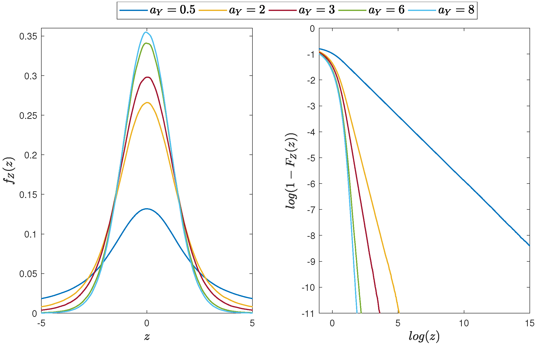
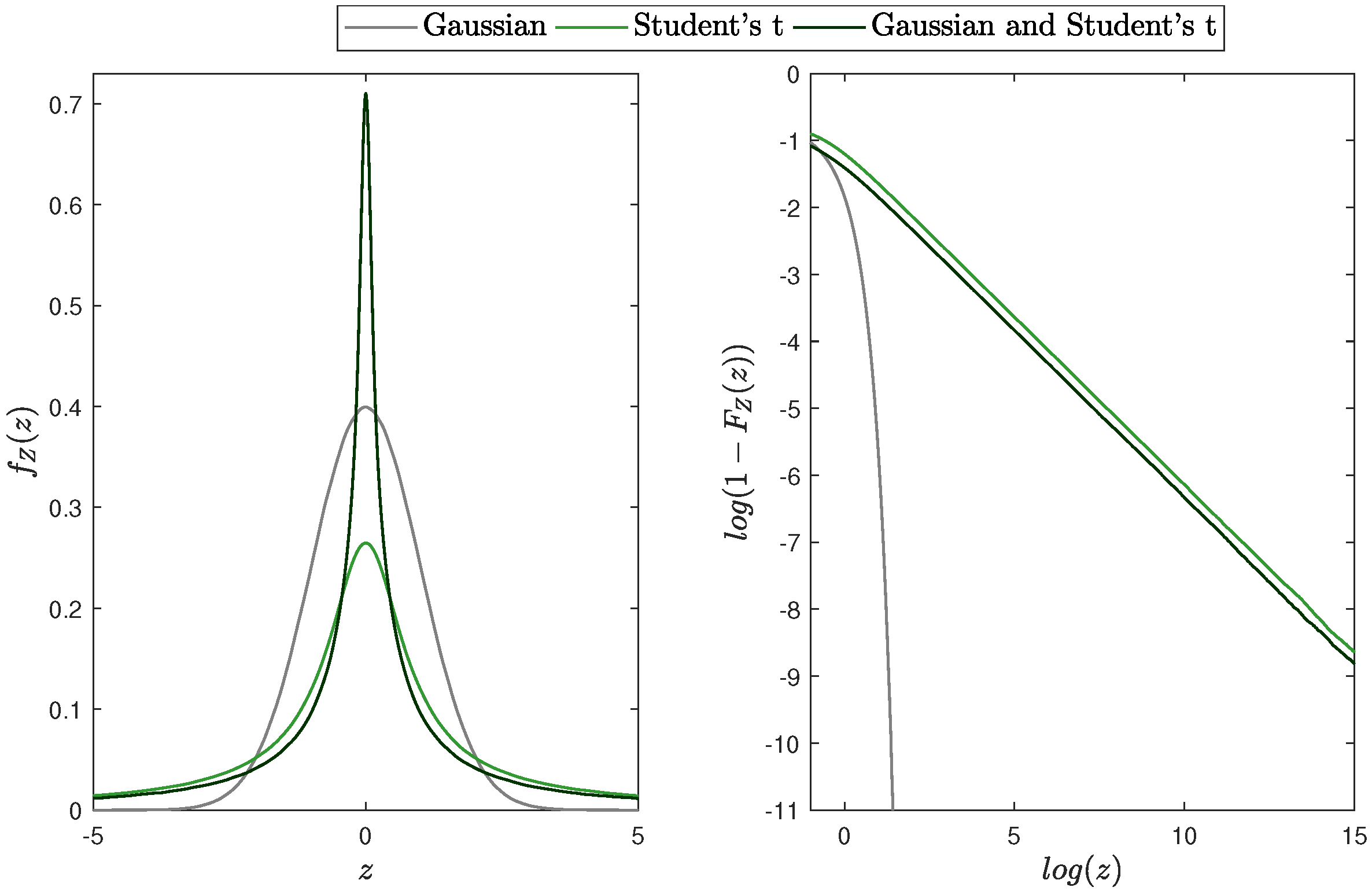
In Figure 7, we plot the PDF and the corresponding distribution tail of the random variable Z that is a product of two independent random variables from the standard Gaussian (i.e., $N(0,1)$) and Student’s t distributions for different values of the parameter $n_Y$. The resulting distribution is symmetric around zero. The shape of its tail is clearly dependent on the value of the parameter $n_Y$. For larger values of $n_Y$, the tails are close to the Gaussian ones, while, for lower $n_Y$, they become much heavier, resembling rather the Student’s t tails. These three distributions, namely, the Gaussian, Student’s t and their product, are compared in Figure 8. One can see that the product has a lighter tail than the Student’s t distributed random variable but a heavier tail than the Gaussian one.

Figure 7. Distribution of the product of two independent random variables from the Gaussian and Student’s t distribution with ${\mu }_X=0$ and ${\sigma }_X=1$ and different values of $n_Y$ parameter. (Left panel): the PDF of the random variable Z. (Right panel): the distribution tail for the random variable Z (in log-log scale).

Figure 8. (Left panel): the PDF of the random variables X (Gaussian), Y (Student’s t) and Z. (Right panel): the distribution tail’s for X, Y and Z. The parameters are equal to: ${\mu }_X=0$ and ${\sigma }_X=1$ and $n_Y=0.5$.

4.3. Product of Log-Normal and Student’s t Distributed Random Variables

In this part, we assume that the one-dimensional random variable X has the log-normal distribution with parameters ${\mu }_X=0$ and ${\sigma }_X>0$, while the one-dimensional random variable Y has the Student’s t distribution with the PDF given in Equation (19) with $n_Y>0$. We assume that X and Y are independent. Using Equation (3), one obtains that the PDF of the random variable Z is given by

$$\begin{array}{cc}\hfill f_Z\left(z\right)& =\frac{\mathsf{\Gamma }\left(\frac{n_Y+1}{2}\right)}{\pi {\sigma }_X\sqrt{2n_Y}\mathsf{\Gamma }\left(\frac{n_Y}{2}\right)}{\int }_0^{\infty }\frac{1}{x^2}exp\left\{-\frac{{log}^2\left(x\right)}{2{\sigma }_X^2}\right\}{\left(1+\frac{z^2}{n_Y{x}^2}\right)}^{-\frac{n_Y+1}{2}}dx.\hfill \end{array}$$

(31)

The PDF given in Equation (31) has no closed form representation and requires numerical calculations. However, using the independence assumption, one can easily show that

$$\mathbb{E}\left(Z\right)=0,\mathbb{V}\mathrm{ar}\left(Z\right)=\frac{n_Y}{n_Y-2}exp\left\{2{\sigma }_X^2-1\right\},$$

(32)

when $n_Y>2$. Similarly as for the Gaussian-Student’s t case, the variance decreases to the variance of X with $n_Y\to \infty$.

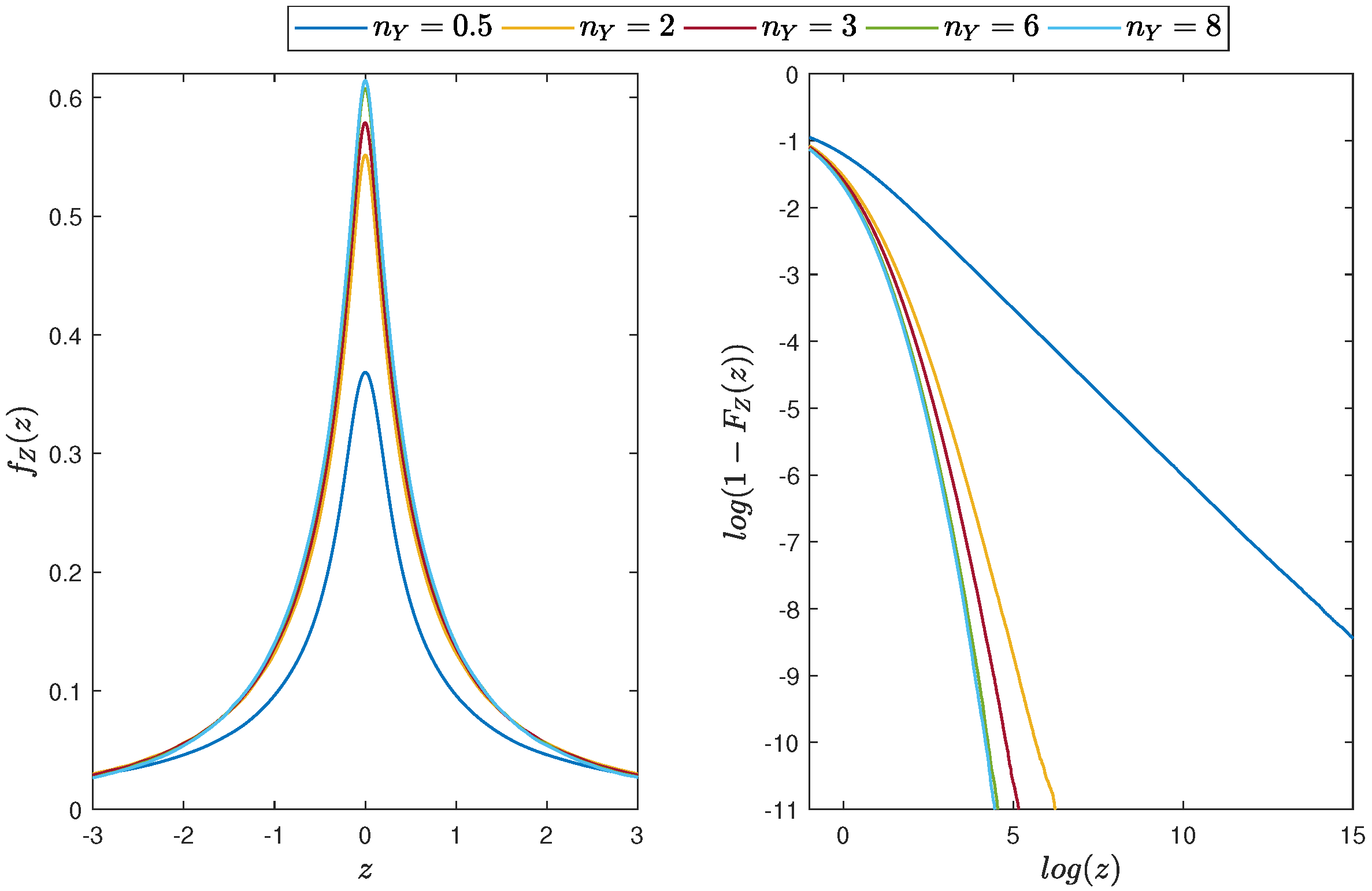
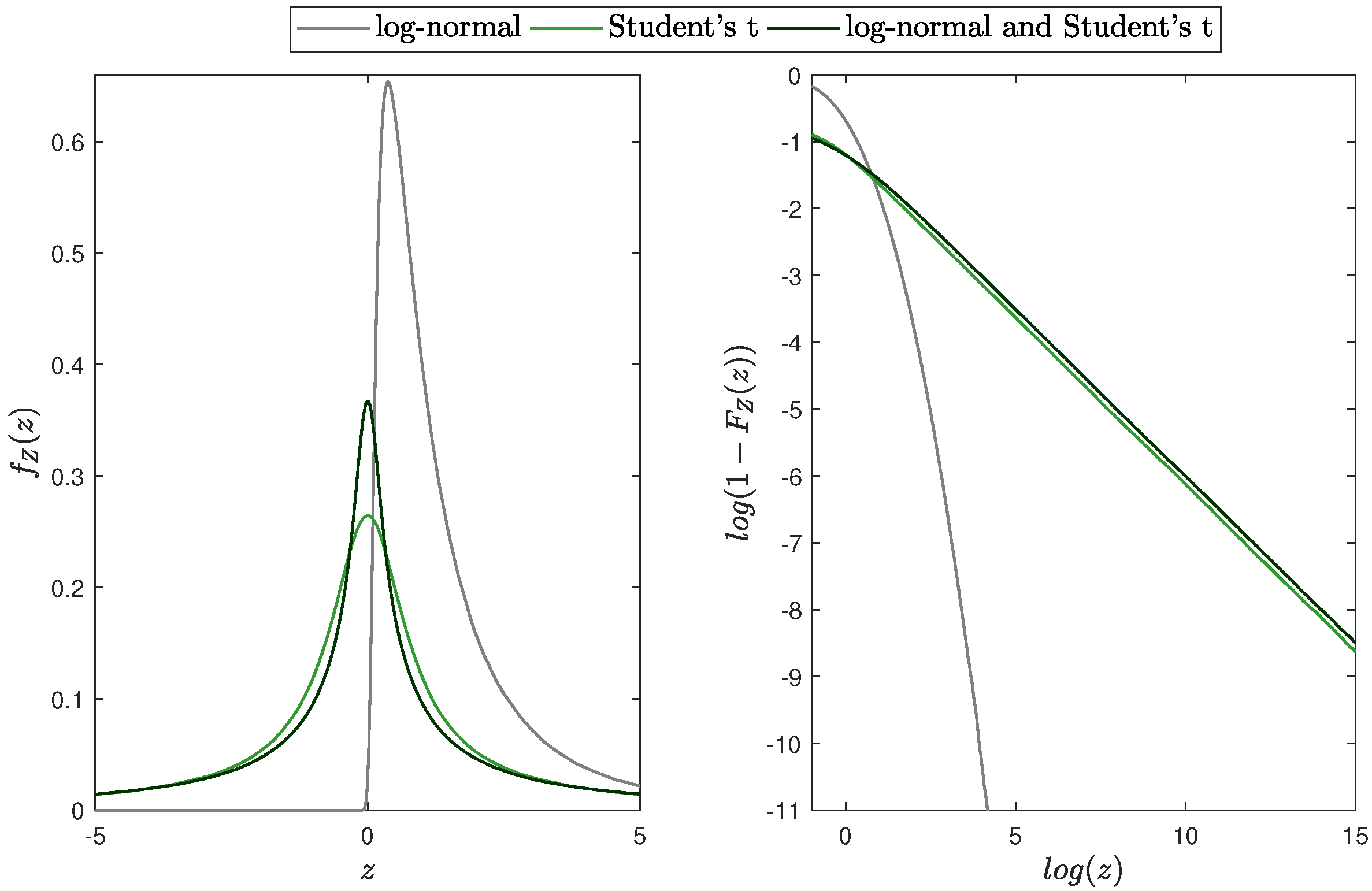
In Figure 9, we plot the PDF and the corresponding distribution tail of the random variable Z for different values of the $n_Y$ parameter, while, in Figure 10, we show a comparison of these three distributions. Similarly as for the Gaussian-Student’s t case (see Figure 7), the tail behaviour is dominated by the Student’s t distribution. However, here the effect in the tails is strengthened by the log-normal distribution.

Figure 9. Distribution of the product of two independent random variables from the log-normal and Student’s t distribution with ${\mu }_X=0$ and ${\sigma }_X=1$ and different values of $n_Y$ parameter. (Left panel): the PDF of the random variable Z; (Right panel): the distribution tail for the random variable Z (in log-log scale).

Figure 10. (Left panel): the PDF of the random variables X (log-normal), Y (Student’s t) and Z. (Right panel): the distribution tails. The parameters are: ${\mu }_X=0$ and ${\sigma }_X=1$ and $n_Y=0.5$.

5. Parameters Estimation–Simulation Study

Based on the formulas for the PDF, $f_Z\left(z\right)$, derived in the previous sections, we illustrate how the parameters of the product distribution can be estimated. To this end, we simulate samples of random vectors $((X_1,Y_1),(X_2,Y_2),\dots ,(X_N,Y_N))$ from the analyzed distributions and calculate the product of each simulated pair, $Z_i=X_i{Y}_i,i=1,2,\dots ,N$. The Gaussian random vectors are generated using the Cholesky decomposition. The simulation of the vectors from the log-normal and dependent Student’s t distribution is based on the relation with the Gaussian distribution. In the case of dependent Pareto variables, the method based on conditional distributions is used, based on the fact that $F_{X,Y}(x,y)=F_X\left(x\right)F_{Y\mid X}(y\mid x)$. First, X is generated using the marginal distribution $F_X\left(x\right)$. Next, Y is generated using the conditional distribution $F_{Y\mid X}(y\mid x=X)$ with X from the first step. For both steps, the inverse CDF method is applied. The independent Student’s t, independent Pareto, Gaussian-Student’s t and Gaussian-Pareto vectors simulation is based on the corresponding one-dimensional distributions.

The estimation of parameters is based on the maximum likelihood method. Thus, we have

$$\widehat{\mathsf{\Theta }}={\mathrm{argmax}}_{\mathsf{\Theta }}L(Z_1,Z_2,\dots .,Z_N;\mathsf{\Theta })={\mathrm{argmax}}_{\mathsf{\Theta }}\prod _{i=1}^N{f}_Z(Z_i;\mathsf{\Theta }),$$

(33)

where $\mathsf{\Theta }$ is the vector of parameters and $f_Z\left(z\right)$ is the corresponding product probability density function. Since analytical solutions do not exist in any of the considered cases, the maximization is performed numerically. Note that the scale parameters of the individual marginal distributions can not be inferred separately from the product, as they jointly yield the scale of the resulting one-dimensional variable, e.g., for the independent Pareto ${\theta }_X{\theta }_Y$.

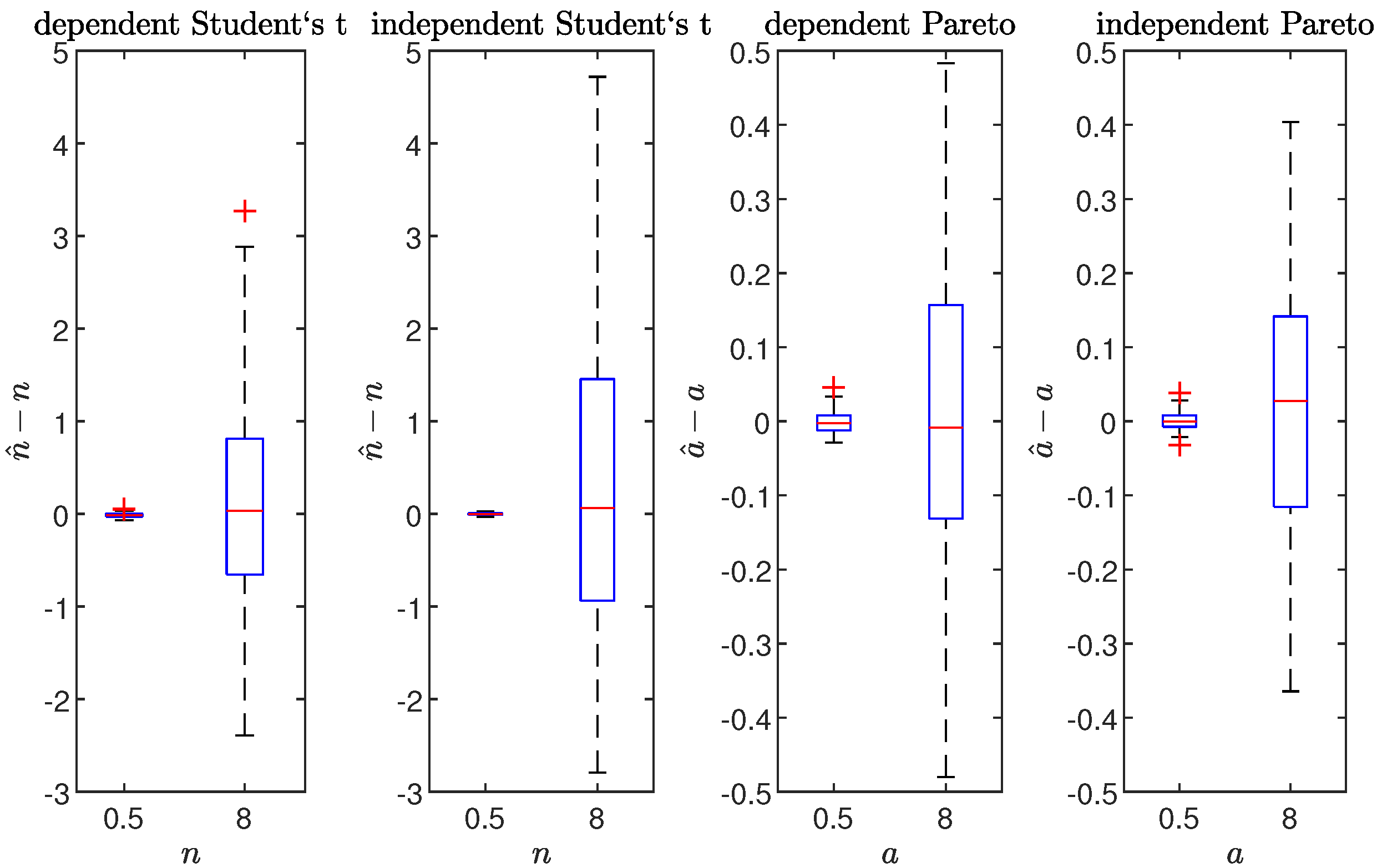
In Figure 11, we plot the boxplots of the errors of the shape parameter estimation for the product of the Student’s t (i.e., $\widehat{n}-n$) and Pareto (i.e., $\widehat{a}-a$) distributions. The dependent variables case (see Equation (21) for Student’s t and Equation (7) for Pareto) as well as the independent one (see Equation (22) for Student’s t and (8) for Pareto) are considered. The other parameters are set to $\rho =0$, and ${\theta }_X={\theta }_Y=1$. In the independent Pareto case, the same shape parameter for both variables, $a_X=a_Y=a$, is considered. The boxplots are plotted for two simulated values of the shape parameter, namely, $n=0.5$ or $n=8$ and $a=0.5$ or $a=8$.

Figure 11. Boxplots of the errors of the degrees of freedom estimator, $\widehat{n}$ and the tail parameter, $\widehat{a}$, for the Student’s t and Pareto distribution products, respectively. (Left panels): results for the dependent and independent Student’s t distribution with $\rho =0$ and $n=0.5$ or $n=8$. (Right panels): results for the dependent and independent Pareto distribution with ${\theta }_X={\theta }_Y=1$ and $a=a_X=a_Y=0.5$ or $a=a_X=a_Y=8$. The length of each sample was equal to 1000, while the number of repetitions was equal to 100.

The obtained error distribution is spread around 0, with much larger deviations in the lighter tails case (i.e., $n=8$ and $a=8$). Such an effect might be caused by the fact that for larger values of the shape parameters the differences between distributions become smaller. In the case of the Student’s t distribution, the errors are not symmetric around zero with more cases of overestimation of the parameter n. In the case of the Pareto distribution, there is no visible asymmetry.

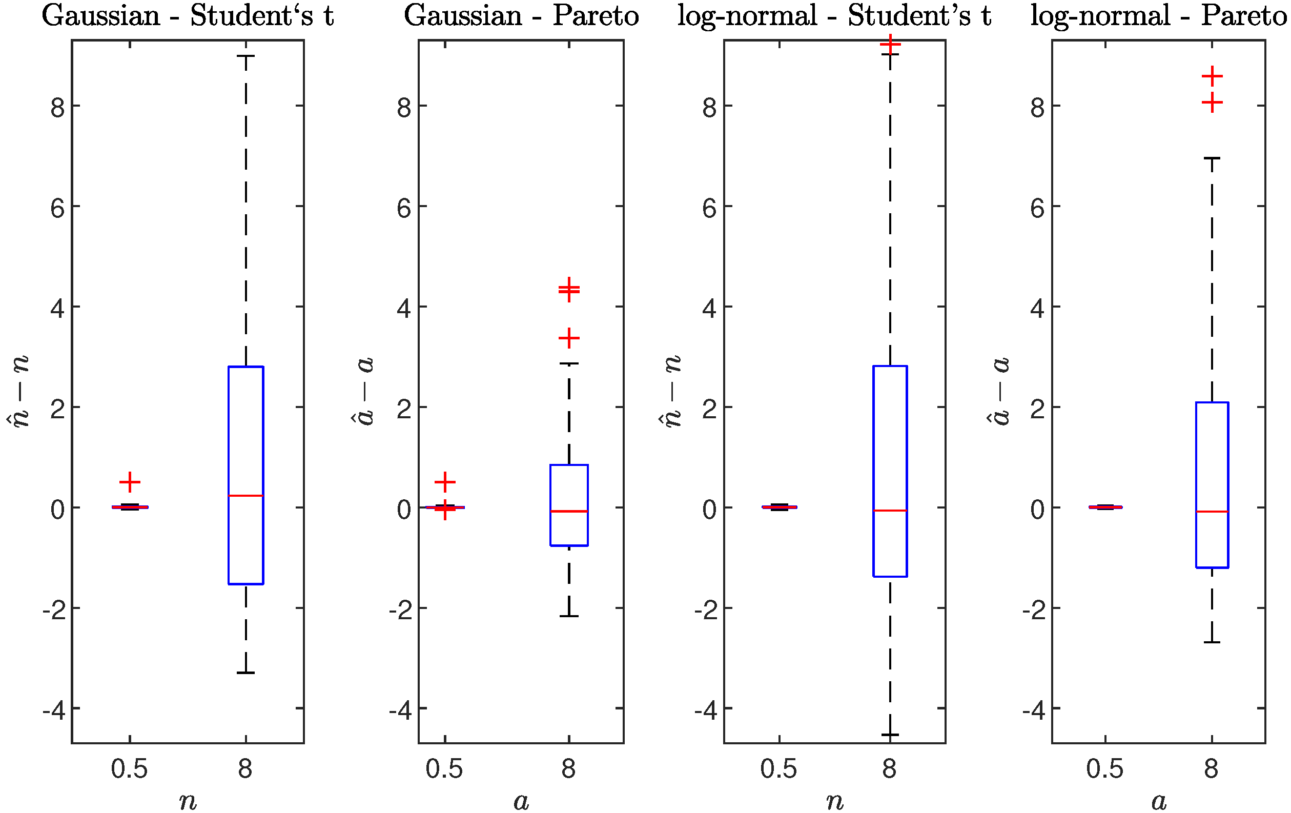
Finally, in Figure 12, we plot the boxplots of the errors of the shape parameters for the products of different marginal distributions, namely, the Gaussian—Student’s t, the Gaussian-Pareto, the log-normal—Student’s t and the log-normal—Pareto case. For the Gaussian and log-normal distributions, we assume ${\mu }_X=0$ and ${\sigma }_X=1$, while the scale parameter of the Pareto distribution is equal to ${\theta }_Y=1$. The errors are analyzed in two cases representing the infinite- ($n=0.5$ for Student’s t distribution or $a_Y=0.5$ for Pareto distribution) as well as finite-variance ($n=8$ for Student’s t distribution or $a_Y=8$ for Pareto distribution). The obtained estimation results are similar to the purely Student’s t or Pareto distributions (see Figure 11). The higher errors are obtained for the higher values of the n and a parameters. Furthermore, the effect of overestimation of the Student’s t degrees of freedom can be noticed.

Figure 12. Boxplots of the errors of the degrees of freedom $\widehat{n}$ and the tail parameter $\widehat{a}$ estimators for the products of the Gaussian or log-normal distribution and Student’s t or Pareto distribution, respectively. The parameters of the Gaussian and log-normal distribution were set to ${\mu }_X=0$ and ${\sigma }_X=1$. The Student’s t distribution was simulated with $n=0.5$ or $n=8$ degrees of freedom, while the Pareto distribution with $\theta =1$ and $a=0.5$ or $a=8$. The length of each sample was equal to 1000, while the number of repetitions was equal to 100.

6. Real Data Application—Distribution of Electricity Transaction Values

In this section, we demonstrate a possible application of the theoretical results discussed in the previous sections to a real-data case. We use the transactions data from the German electricity market settled in the EPEX energy exchange. Each transaction is characterized by two values: the volume of sold energy (in MWh) and the price (in EUR/MWh). The final transaction value, being the amount of the total profit for the energy seller or a total cost for energy buyer, is the product of these two variables. Hence, knowing the product distribution is important for profit/costs planning in energy companies.

The data come from a continuous intraday electricity market, which involves trading of electricity from 3:00 pm on the day before physical delivery up to 5 min before it. A transaction is settled each time two bid and sell offers meet. Hence, each data point corresponds to a different offer and usually a different market participant, being in fact a transaction on different products with the same delivery date. Therefore, we assume that the sample points are independent. One of the main characteristics of the electricity market is its seasonality on the yearly, weekly, and daily level [76]. To avoid the possible influence of the transaction time on its distribution, we analyze separately the transactions being settled in different hours, so the data refer to different market participants approximately at the same time. The data points within one hour are assumed to be identically distributed.

We analyze vectors $\{(x_1,y_1),(x_2,y_2),\dots ,(x_n,y_n)\}$, where $x_i$ is the volume and $y_i$ is the price of the i-th transaction within a given hour and n is the number of transactions during this hour. We also analyze a sample of the transaction values being a product of each $x_i$ and $y_i$, i.e., $\{x_1{y}_1,x_2{y}_2,\dots ,x_n{y}_n\}$. For an illustration, we have chosen two representative hours, namely, hour 14 from 20 December 2020 and hour 8 from 15 March 2020. The first case shows a typical picture that is observable for most hours, while the second case illustrates the less frequent but typical for the German electricity market situation, where some of transaction prices are negative. Negative prices are a unique feature of electricity markets caused by the limited ability to store electricity and the fast development of production from renewable energy sources [77]. If there is a short-term oversupply of electricity due, for example, to wind or solar production, the producers from conventional energy sources might be willing to pay for the reception of electricity instead of stopping the production units.

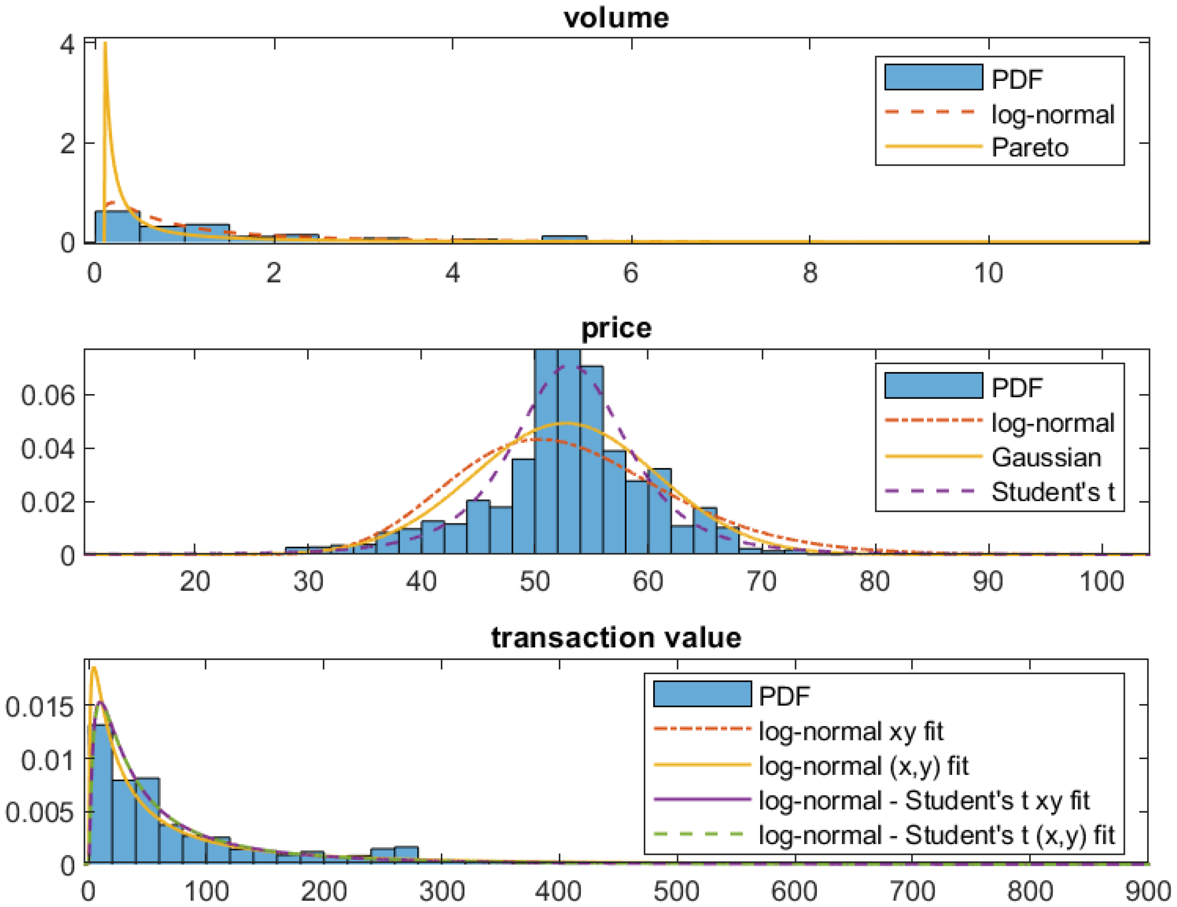
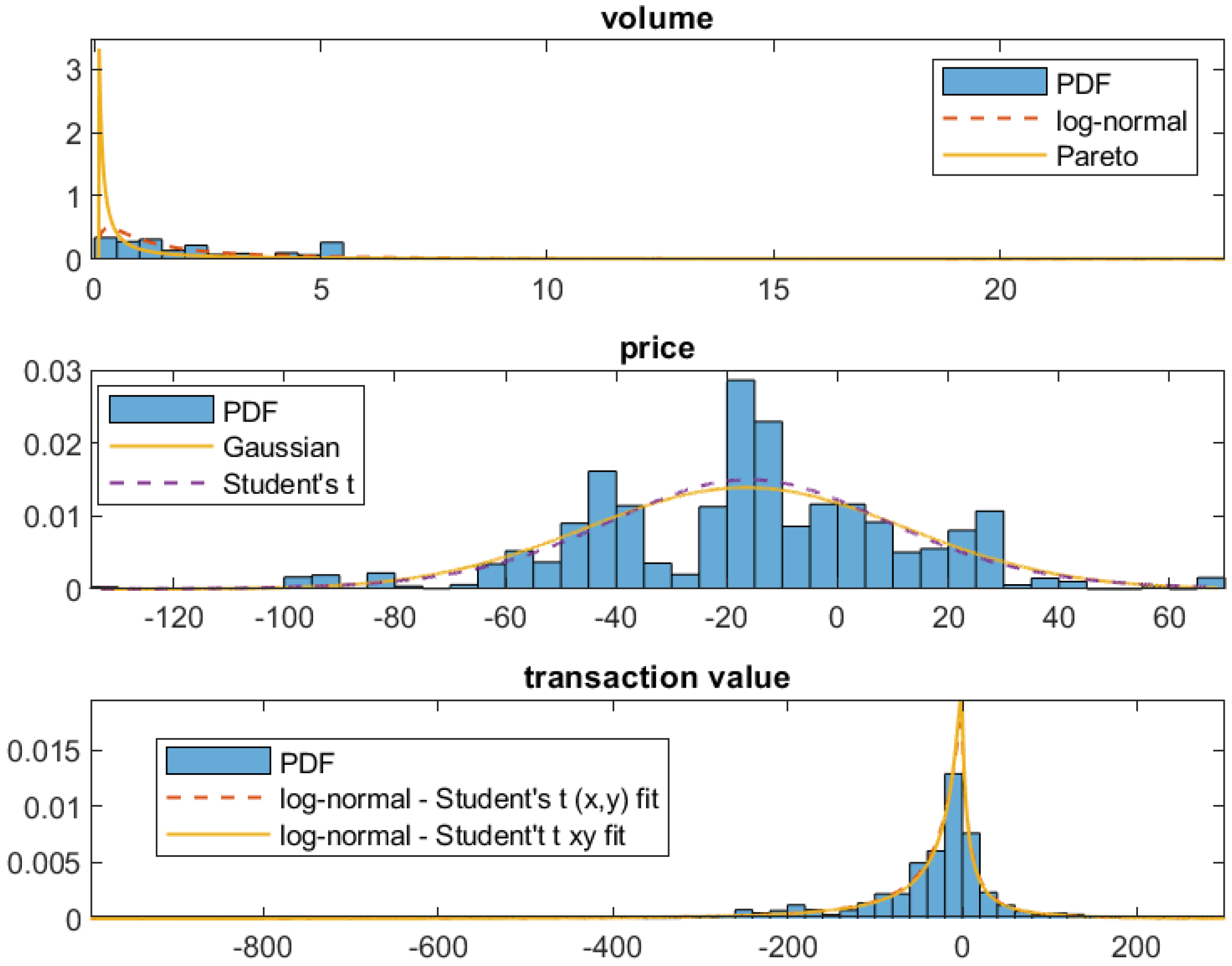
The corresponding PDFs are plotted in Figure 13 and Figure 14 for 20 December and 15 March, respectively. The parameters of the considered distributions are estimated using the maximum likelihood method with formulas for the corresponding PDFs. If the formulas are not given explicitly, they are calculated numerically. There are 4963 and 4608 observations for 20 December and 15 March, respectively. The correlation between the volume and price samples is not significant. Precisely, it is equal to −0.0011 for the transactions on 20 December and −0.0261 for the transactions on 15 March. The corresponding p-values for the t-test on zero correlation are equal to 0.9388 and 0.0765, respectively. Hence, we assume that the corresponding X and Y random variables are not correlated. Since the volume can not be negative, the only distributions from the ones analyzed in the paper that can be fitted to the volume sample are the log-normal and Pareto. For the price sample, the Gaussian, log-normal (for positive data) and Student’s t with location and scale parameters are fitted. The resulting densities are plotted in the corresponding panels of Figure 13 and Figure 14.

Figure 13. Probability distribution of the volume (top panel), price (middle panel) and their product, i.e., the transaction value (bottom panel) from the continuous intraday energy market data on 20 December 2020, hour 14. The fitted PDFs are also plotted. The transaction value densities are fitted in two ways: separately to the x (price) and y (volume) data (denoted by ‘$(x,y)$ fit’) or to the product $xy$ (transaction value) data (denoted by ‘$xy$ fit’).

Figure 14. Probability distribution of the volume (top panel), price (middle panel) and their product, i.e., the transaction value (bottom panel) from the continuous intraday energy market data on 15 March 2020, hour 8. The fitted PDFs are also plotted. The transaction value densities are fitted in two ways: separately to the x (price) and y (volume) data (denoted by ‘$(x,y)$ fit’) or to the product $xy$ (transaction value) data (denoted by ‘$xy$ fit’).

For both analyzed hours, the log-normal distribution density function resembles the shape of the volume histogram. On the other hand, the Pareto distribution clearly overestimates the probability of small volumes. Hence, for the product analysis, we will only consider the log-normal distribution for the first coordinate. Looking at the price distribution for the data from hour 14 on 20 December 2020 (see Figure 13), we can observe that only the Student’s t PDF resembles the shape of the obtained histogram, especially around the mean, where the Gaussian and log-normal probabilities are underestimated.

The picture for the second considered data set, i.e., the price distribution from hour 8 on 15 March 2020 (see Figure 14), is different. First, there is a significant probability of obtaining negative values. Hence, in this case, we do not fit the log-normal distribution, which can take only positive values. Second, the Gaussian and the Student’s t PDF produce a similar fit. Recall that, with increasing degrees of freedom in the latter case, the distribution tends to the Gaussian one. The tails for this hour are lighter than for the 20 December data. Overall, from the set of the considered distributions, the Student’s t is best fitting the prices from both analyzed hours.

Next, we analyze the resulting product, i.e., the transaction value distribution. To this end, we proceed in two ways. Firstly, we use the parameters estimated for the one-dimensional samples of the random variables X and Y (i.e., volumes and prices) and use the formulas for the product PDF derived in in the previous sections. Based on the results obtained for the one-dimensional samples, we show only the product of log-normal distribution or log-normal and Student’s t distribution (log-normal-Student’s t). Secondly, we also fit the derived PDFs to the sample of the product $XY$. We can observe that the final product PDF obtained by these two ways in the case of log-normal-Student’s t overlaps and resembles the shape of the sample histogram, confirming a good fit. As mentioned before, due to the negative prices apparent in the second analyzed hour, the log-normal distribution can be fitted only to the first dataset. In this case, we can observe a discrepancy between the density obtained using the $(X,Y)$ coordinates and its product $XY$. Comparing the obtained shapes of the distribution for both hours, we can see a clear difference between these cases. The transaction values for hour 8 on 15 March 2020 take both negative and positive values, with long left tails of the distribution. On the other hand, there are no negative transaction values for hour 14 on 20 December 2020, and the distribution is right skewed.

The comparison of the fitted distributions is further evaluated based on the distance between the corresponding cumulative distribution functions (CDFs). We calculate two-sample Kolmogorov–Smirnov statistics (KS); see, e.g., [78], which is the maximal distance between empirical CDFs from two samples. Here, these are the analyzed dataset and the sample simulated from the corresponding distribution. The KS statistic can be also used for the goodness-of-fit testing. However, for large samples, even small differences between distributions lead to rejection of the hypothesized distribution. Here, all of the considered distributions are rejected at 0.01 significance level, except for the transaction values on 15 March, for which the rejection rate for 1000 simulated samples is $78\%$. We also calculate the root mean square error (RMSE) between the empirical CDFs. Note that the theoretical distribution is derived from simulations, since, for most of the considered cases, the PDFs are not given in closed form. In Table 1, we give the mean values of the KS statistics and RMSE calculated from 1000 simulations. For the comparison of the considered distributions, we also calculate the Kullback–Leibler divergence (KLD), see, e.g., [79], i.e., ${\int }_{\mathrm{R}}p\left(x\right)log\left(\frac{p\left(x\right)}{q\left(x\right)}\right)dx$, where p and q are the compared PDFs. Here, $p(·)$ is the histogram estimated from the sample, $q(·)$ is the PDF of the considered distribution, while the integral is calculated numerically. The obtained values are also given in Table 1.

Table 1. Values of the Kolmogorov–Smirnov (KS) statistics, root mean square error (RMSE) and Kullback–Leibler divergence between the data and the considered distributions. KS statistic and RMSE were calculated as the means from 1000 simulated samples from the considered distributions.

20 December
Variable	Distribution	KS statistic	RMSE	KLD
Volume	log-normal	0.0810	0.0359	0.1367
	Pareto	0.2263	0.1350	0.5717
Price	log-normal	0.1719	0.0813	3.1737
	Gaussian	0.1305	0.0560	2.5211
	Student’s t	0.0523	0.0206	2.5304
Value	log-normal (x, y)	0.0501	0.0247	0.0819
	log-normal xy	0.0498	0.0247	0.0208
	log-normal—Student’s t (x, y)	0.0487	0.0242	0.0214
	log-normal—Student’s t xy	0.0500	0.0245	0.0214
15 March
Volume	log-normal	0.0952	0.0501	0.2868
	Pareto	0.2881	0.1702	0.9211
Price	Gaussian	0.1014	0.0333	1.4262
	Student’s t	0.0891	0.0308	1.4707
Value	log-normal—Student’s t (x, y)	0.0414	0.0167	1.4370
	log-normal—Student’s t xy	0.0369	0.0148	1.4202

As can be observed in Table 1, for transactions on 20 December, the smallest difference from the considered distributions is, indeed, obtained for the log-normal—Student’s t case. The Pareto distribution for the volume is outperformed by the log-normal one, according to each of the three measures. For the price distribution, the sample CDF is the closest to the Student’s t CDF according to the KS statistic and RMSE values. Only the KLD value yields similar results for the Gaussian PDF. The product distributions fitted to transaction values yield similar levels of the KS statistic, RMSE and KLD except for log-normal distribution fitted separately to prices and volumes, which gives the worst results. For transactions on 15 March, again, the log-normal distribution outperforms the Pareto one for the volume data according to all considered measures. The Student’s t distribution estimated from the sample of prices is close to the Gaussian one. Overall, only the log-normal-Student’s t case from the considered distributions set is flexible enough to be reasonably applied to both analyzed representative hours.

7. Conclusions

In this paper, we have discussed the distribution of a random variable that is a product of two continuous random variables when at least one of them belongs to the heavy-tailed class of distributions. The considered distributions are Pareto and Student’s t. The main attention was paid to the influence of the parameters of the marginal random variables on the final product characteristics. For both cases, we have discussed how the dependency between the marginal random variables (when the two random variables have the same distribution) influences the probabilistic properties of the product. Next, we have discussed the product of the random variables coming from different classes of distributions, for which we have derived the explicit form of the PDF for the Gaussian-Pareto and the log-normal-Pareto case and studied the resulting tail behavior. The derived as well as recalled formulas for the considered distributions are gathered in Table 2 and Table 3, for the Pareto and Student’s t distributions, respectively.

Table 2. Summary of the formulas for PDFs, $f_Z$, its asymptotic behaviour for $z\to \infty$ and two first moments, $\mathbb{E}\left(Z\right)$ and $\mathbb{V}ar\left(Z\right)$ for the considered products with Pareto distribution.

Multivariate Pareto

$f_Z\left(z\right)=(a+1)a{\left({\theta }_X{\theta }_Y\right)}^{a+1}\underset{{\theta }_X}{\overset{\frac{z}{{\theta }_Y}}{\int }}\frac{1}{x}{({\theta }_{Y}x+{\theta }_X\frac{z}{x}-{\theta }_X{\theta }_Y)}^{-a-2}dx,z>{\theta }_X{\theta }_Y$

Independent Pareto

$f_Z\left(z\right)=\left\{\begin{array}{c}{a}_X{a}_Y\left(\frac{z^{-a_X-1}{\left({\theta }_X{\theta }_Y\right)}^{a_X}}{a_Y-a_X}+\frac{z^{-a_Y-1}{\left({\theta }_X{\theta }_Y\right)}^{a_Y}}{a_X-a_Y}\right){𝟙}_{\{z>{\theta }_X{\theta }_Y\}},\mathrm{if}{a}_X\ne a_Y\hfill \\ a^2\left({\theta }_X{\theta }_Y\right)z^{-a-1}log\left(\frac{z}{{\theta }_X{\theta }_Y}\right){𝟙}_{\{z>{\theta }_X{\theta }_Y\}},\mathrm{if}{a}_X=a_Y=a\hfill \end{array}\right.$

$\mathbb{E}\left(Z\right)=\frac{{\theta }_X{\theta }_Y{a}_X{a}_Y}{(a_X-1)(a_Y-1)}\mathrm{for}{a}_X,a_Y>1$

$\mathbb{V}\mathrm{ar}\left(Z\right)={\theta }_X^2{\theta }_Y^2{a}_X{a}_Y\left[\frac{{(a_X-1)}^2+{(a_Y-1)}^2-1}{(a_X-2)(a_Y-2){(a_X-1)}^2{(a_Y-1)}^2}\right]\mathrm{for}{a}_X,a_Y>2$

Gaussian-Pareto

$f_Z\left(z\right)=\frac{a_Y{\theta }_Y^{a_Y}{\sigma }_X^{a_Y}}{\sqrt{2\pi }\mid z{\mid }^{a_Y+1}}{2}^{(a_Y-1)/2}\gamma \left(\frac{a_Y+1}{2},\frac{z^2}{2{\sigma }^2{\theta }_Y^2}\right)$

$f_Z\left(z\right)\sim \frac{a_Y{\theta }_Y^{a_Y}{\sigma }_X^{a_Y}}{\sqrt{2\pi }}{2}^{(a_Y-1)/2}\mathsf{\Gamma }\left(\frac{a_y+1}{2}\right)z^{-a_Y-1}\mathrm{for}z\to \infty$

$\mathbb{E}\left(Z\right)=0\mathrm{for}{a}_Y>1$

$\mathbb{V}\mathrm{ar}\left(Z\right)=\frac{{\left({\theta }_Y{\sigma }_X\right)}^2{a}_Y}{(a_Y-2)}\mathrm{for}{a}_Y>2$

Log-normal-Pareto

$f_Z\left(z\right)=\frac{a_Y{\theta }_Y^{a_Y}exp\left\{\frac{a_Y^2{\sigma }_X^2}{2}\right\}}{z^{a_Y+1}}\mathsf{\Phi }\left(\frac{log(z/{\theta }_Y)-a_Y{\sigma }_X^2}{{\sigma }_X}\right){𝟙}_{\{z>0\}}$

$f_Z\left(z\right)\sim a_Y{\theta }_Y^{a_Y}exp\left\{\frac{a_Y^2{\sigma }_X^2}{2}\right\}{z}^{-a_Y-1}\mathrm{for}z\to \infty$

$\mathbb{E}\left(Z\right)=\frac{{\theta }_Y{a}_Y}{a_Y-1}exp\left\{\frac{{\sigma }_X^2}{2}\right\}\mathrm{for}{a}_Y>1$

$\mathbb{V}\mathrm{ar}\left(Z\right)=\frac{{\theta }_Y^2{a}_{Y}exp\left\{2{\sigma }_X^2\right\}}{{(a_Y-1)}^2}\left(\frac{1}{a_Y-2}+a_Y-a_{Y}exp\left\{-{\sigma }_X^2\right\}\right)\mathrm{for}{a}_Y>2$

Table 3. Summary of the formulas for PDFs, $f_Z$, its asymptotic behaviour for $z\to \infty$ and two first moments, $\mathbb{E}\left(Z\right)$ and $\mathbb{V}ar\left(Z\right)$ for the considered products with Student’s t distribution.

Multivariate Student’s t

$f_Z\left(z\right)=\frac{1}{\pi \sqrt{1-{\rho }^2}}{\int }_0^{\infty }\frac{1}{x}{\left[1+\frac{x^2-2\rho z+\frac{z^2}{x^2}}{n(1-{\rho }^2)}\right]}^{-\frac{n+2}{2}}dx$

Independent Student’s t

$f_Z\left(z\right)=\frac{2\mathsf{\Gamma }\left(\frac{n_X+1}{2}\right)\mathsf{\Gamma }\left(\frac{n_Y+1}{2}\right)}{\sqrt{n_X{n}_Y}\pi \mathsf{\Gamma }\left(\frac{n_X}{2}\right)\mathsf{\Gamma }\left(\frac{n_Y}{2}\right)}{\int }_0^{\infty }\frac{1}{x}{\left(1+\frac{x^2}{n_X}\right)}^{-\frac{n_X+1}{2}}{\left(1+\frac{z^2}{x^2{n}_Y}\right)}^{-\frac{n_Y+1}{2}}dx$

$\mathbb{E}\left(Z\right)=0\mathrm{for}{n}_X,n_Y>1$

$\mathbb{V}ar\left(Z\right)=\frac{n_X{n}_Y}{(n_X-2)(n_Y-2)}\mathrm{for}{n}_X,n_Y>2$

Gaussian-Student’s t

$f_Z\left(z\right)=\sqrt{\frac{1}{2n_Y}}\frac{\mathsf{\Gamma }(\frac{n_Y}{2},\frac{1}{2})}{B(\frac{n_Y}{2},\frac{1}{2})}\psi \left(\frac{n_Y}{2}+\frac{1}{2},1,\frac{z^2}{2{\sigma }_X^2{n}_Y}\right)$

$f_Z\left(z\right)\sim {\left(2{\sigma }_X^2{n}_Y\right)}^{\frac{n_Y+1}{2}}{z}^{-n_Y-1}$

$\mathbb{E}\left(Z\right)=0\mathrm{for}{n}_Y>1$

$\mathbb{V}ar\left(Z\right)=\frac{n_Y}{n_Y-2}{\sigma }_X^2\mathrm{for}{n}_Y>2$

Log-normal-Student’s t

$f_Z\left(z\right)=\frac{\mathsf{\Gamma }\left(\frac{n_Y+1}{2}\right)}{\pi {\sigma }_X\sqrt{2n_Y}\mathsf{\Gamma }\left(\frac{n_Y}{2}\right)}{\int }_0^{\infty }\frac{1}{x^2}exp\left\{-\frac{{log}^2\left(x\right)}{2{\sigma }_X^2}\right\}{\left(1+\frac{z^2}{n_Y{x}^2}\right)}^{-\frac{n_Y+1}{2}}dx$

$\mathbb{E}\left(Z\right)=0\mathrm{for}{n}_Y>1$

$\mathbb{V}ar\left(Z\right)=\frac{n_Y}{n_Y-2}exp\left\{2{\sigma }_X^2-1\right\}\mathrm{for}{n}_Y>2$

The theoretical results were applied in the proposed estimation methodology. We used a general approach based on the maximum likelihood technique. The presented Monte Carlo simulations clearly indicate the effectiveness of the algorithm. Finally, the real data analysis was presented. Based on the data from continuous trading on the German energy market, we have shown that, from the considered distributions, the log-normal and Student’s t one yields the best fit to the transaction values. Since the transaction value is the final profit/cost for a trader, finding a proper density describing its distribution, which is also consistent with the prices and volumes data, can help an energy market participant in strategy planning.

8. Discussion

Product distributions occur naturally also in other financial contexts. Another potential application of the proposed methodology could be the market risk area in metals and mining business. Mining companies are exposed to two or more market risk factors, like metal prices and currency exchange rates. These factors’ behavior is often characterized by non-Gaussian distributions, which can be reflected by that discussed in this paper, Student’s t distribution. From a business perspective of an international mining company, which trades the excavated resources in different than national currency, it is valuable to analyse the selling price also in the national currency that is a product of the commodity price (usually quoted in USD) and USD/national currency exchange rate. A case study related to the modelling of the copper prices for a Polish mining company one can find in [1]. It has been shown that the behavior of metal price in PLN exhibits specific characteristics that follow directly from the properties of the individual variables and dependence between them. These properties need to be reflected in optimizing strategies aimed at mitigation of the unacceptable market risk for a company.

From the theoretical point of view, the problem analyzed in this paper can be considered as a special case of a general issue related to the time series (or stochastic process) that arises as a product of two other time series. This problem is rarely discussed in the literature (see e.g., [80,81]), but it seems to be interesting, especially from the practical point of view. Obviously, in some economical applications, the variable of main interest is the product of time series describing time-dependent market variables, like, e.g., the cost, being the product of price and volume. Thus, our future study will be related to this issue. It should be noted that, in the examination of the product of random variables, the main attention is usually paid to its probabilistic properties (i.e., probability distribution) and the analysis on how the characteristics of the individual random variables influence the final product’s properties. In the case when the individual variables are components of some time series, the main attention is paid on the dependence structure of the final product and the analysis how the auto- or cross- dependence between the variables influence the new time series. An interesting example can be the product of the components of the multi-dimensional time series describing time-dependent economical variables.

In future study, we also plan to examine more complicated issues, namely the product of components from a multivariate continuous-time stochastic process. From a theoretical point of view, this issue seems to be interesting, especially when the stochastic process under consideration is non-Gaussian and its marginal distributions are heavy-tailed and have infinite variance. Similarly as in the case of product of time series components, here the dependence structure may be the most important issue. However, in case of the infinite-variance distributions of the marginal random variables, the dependence needs to be described in the language of appropriate measures. This point needs to be addressed in the future study as well.

Appendix A.1. Product of Two Gaussian Distributed Random Variables

The two-dimensional Gaussian distributed random random vector $(X,Y)$ has the following PDF [82]:

$$f_{X,Y}(x,y)=\frac{exp\left\{-\frac{1}{2(1-{\rho }^2)}\left[\frac{{(x-{\mu }_X)}^2}{{\sigma }_X^2}-2\rho \left(\frac{x-{\mu }_X}{{\sigma }_X}\right)\left(\frac{y-{\mu }_Y}{{\sigma }_Y}\right)+\frac{{(y-{\mu }_Y)}^2}{{\sigma }_Y^2}\right]\right\}}{2\pi {\sigma }_X{\sigma }_Y\sqrt{1-{\rho }^2}},$$

(A1)

where $x,y\in \mathbb{R}$, $\rho \in (-1,1)$ is the correlation coefficient between random variables X and Y; ${\mu }_X,{\mu }_Y\in \mathbb{R}$ are the corresponding expected values, while ${\sigma }_X,{\sigma }_Y>0$ are the corresponding standard deviations. The cases $\rho =1$ or $\rho =-1$ are not considered in this paper. However, they correspond to the situation when $Y=aX$, with $a\in \mathbb{R}$. As a consequence, the product random variable Z has a chi-square distribution with one degree of freedom. It is easy to see that, when $\rho =0$, the PDF of the random vector $(X,Y)$ is just a product of the PDFs of the Gaussian distributed random variables.

For simplicity, we assume that ${\mu }_X={\mu }_Y=0$. In that case, the PDF of the random variable Z defined in (1) is given by [56]

$$f_Z\left(z\right)=\frac{1}{\pi {\sigma }_X{\sigma }_Y\sqrt{1-{\rho }^2}}exp\left\{\frac{\rho z}{{\sigma }_X{\sigma }_Y(1-{\rho }^2)}\right\}{K}_0\left(\frac{\mid z\mid }{{\sigma }_X{\sigma }_Y(1-{\rho }^2)}\right),$$

(A2)

where $z\in \mathbb{R}$, $K_0(·)$ is the Bessel function of the second kind with a purely imaginary argument of zero order. Recall that the family of the modified Bessel functions of the second kind for order v is given by $K_v\left(x\right)={\int }_0^{\infty }exp\{-xcosh\left(t\right)\}cosh\left(vt\right)dt$. The formula for $f_Z(·)$ in the general case with ${\mu }_X={\mu }_Y\in \mathbb{R}$ can be found in [83].

One can show that the PDF given in Equation (A2) corresponds to the variance-gamma distribution PDF: $VG(1,\rho {\sigma }_x{\sigma }_y,{\sigma }_x{\sigma }_y\sqrt{1-{\rho }^2},0)$. The expected value and the variance of Z in the general case are given by [84]

$$\begin{array}{cc}\hfill \mathbb{E}\left(Z\right)& ={\mu }_X{\mu }_Y+\rho {\sigma }_X{\sigma }_Y,\hfill \end{array}$$

(A3)

$$\begin{array}{cc}\hfill Var\left(Z\right)& ={\sigma }_X^2{\mu }_Y^2+{\sigma }_Y^2{\mu }_X^2+{\sigma }_X^2{\sigma }_Y^2+2\rho {\mu }_X{\mu }_Y{\sigma }_X{\sigma }_Y+{\rho }^2{\sigma }_X^2{\sigma }_Y^2.\hfill \end{array}$$

(A4)

It is interesting to note that, for correlated marginal variables, the individual scale parameters, ${\sigma }_X,{\sigma }_Y$ influence also the expected value of the product, $\mathbb{E}\left(Z\right)$, and for central marginal distributions we have $\mathbb{E}\left(Z\right)\ne 0$. On the other hand, if $\rho =0$, then the product expectation is just the product of the individual means, ${\mu }_X,{\mu }_Y$. The variance of the product is equal to the product of individual variances only if ${\mu }_X={\mu }_Y=0$ and the marginal variables are uncorrelated. Otherwise, it is a function of all individual parameters.

Appendix A.2. Product of Two Log-Normally Distributed Random Variables

The two-dimensional log-normally distributed random vector $(X,Y)$ with parameters ${\mu }_X,{\mu }_Y\in \mathbb{R}$, ${\sigma }_X,{\sigma }_Y>0$ and $\rho \in (-1,1)$ is defined in the following way [85]:

$$\begin{array}{c}\hfill (X,Y)=exp\left\{(N_1,N_2)\right\},\end{array}$$

(A5)

where $(N_1,N_2)$ is the Gaussian random vector defined by the PDF in Equation (A1) with the parameters ${\mu }_X,{\mu }_Y,{\sigma }_X,{\sigma }_Y$ and $\rho$. Thus, the marginal random variables X and Y have the representations

$$\begin{array}{c}\hfill X=exp\left\{N_1\right\},Y=exp\left\{N_2\right\}\end{array}$$

(A6)

and in the general case the $\rho$ parameter is the correlation between $N_1$ and $N_2$. This influences also the correlation between X and Y. Indeed, one can easily show that the covariance between X and Y is as follows:

$$\begin{array}{c}\hfill \mathrm{cov}(X,Y)=exp\left\{{\mu }_X+{\mu }_Y+\frac{1}{2}({\sigma }_X^2+{\sigma }_Y^2)\right\}[exp\left\{\rho {\sigma }_X{\sigma }_Y\right\}-1].\end{array}$$

(A7)

The PDF of $(X,Y)$ is given by [86]

$$f_{X,Y}(x,y)=\frac{exp\left\{-\frac{\frac{{(log\left(x\right)-{\mu }_X)}^2}{{\sigma }_X^2}-2\rho \frac{(log\left(x\right)-{\mu }_X)(log\left(y\right)-{\mu }_Y)}{{\sigma }_X{\sigma }_Y}+\frac{{(log\left(y\right)-{\mu }_Y)}^2}{{\sigma }_Y^2}}{2(1-{\rho }^2)}\right\}}{2\pi xy{\sigma }_X{\sigma }_Y\sqrt{1-{\rho }^2}},$$

(A8)

where $x,y>0$. If $\rho =0$, the marginal variables X and Y are independent and the PDF given in (A8) is a product of PDFs of one-dimensional random variables with the log-normal distribution. The cases $\rho =1$ and $\rho =-1$ are not considered in this paper. However, one can notice that, in these cases, the product random variable Z has still the log-normal distribution.

One can show that the random variable Z defined in Equation (1) in the considered case also has one-dimensional log-normal distribution. Indeed, from Equation (A6), one has

$$Z=XY=exp\{N_1+N_2\}.$$

Since $N_1$ and $N_2$ are jointly Gaussian, the random variable $N_1+N_2$ still has the Gaussian distribution with the expected value ${\mu }_X+{\mu }_Y$ and the variance ${\sigma }_X^2+{\sigma }_Y^2+2\rho {\sigma }_X{\sigma }_Y$. Thus, the PDF of Z has the following form:

$$\begin{array}{c}\hfill f_Z\left(z\right)=\frac{1}{\sqrt{2\pi ({\sigma }_X^2+{\sigma }_Y^2+2\rho {\sigma }_X{\sigma }_Y)}z}exp\left\{-\frac{1}{2}\frac{{(log\left(z\right)-{\mu }_X-{\mu }_Y)}^2}{{\sigma }_X^2+{\sigma }_Y^2+2\rho {\sigma }_X{\sigma }_Y}\right\}\end{array}$$

(A9)

for $z>0$. The resulting product distribution is still log-normal with the following parameters: ${\mu }_Z={\mu }_X+{\mu }_Y$ and ${\sigma }_Z^2={\sigma }_X^2+{\sigma }_Y^2+2\rho {\sigma }_X{\sigma }_Y$. Hence, the $\rho$ coefficient influences the scale parameter of the resulting distribution.

Appendix B.1. Proof of Lemma 2

Proof of Lemma 2.

Let us first note that the CDF of Y is given by

$$\begin{array}{c}\hfill F_Y\left(y\right)=1-{\theta }_Y^{a_Y}{y}^{-a_Y},y>{\theta }_Y.\end{array}$$

(A10)

Thus, the CDF of Z takes the form

$$\begin{array}{ccc}\hfill F_Z\left(z\right)& =& P(XY<z)={\int }_{-\infty }^{\infty }P(Yx<z)f_X\left(x\right)dx\hfill \\ & =& \frac{1}{\sqrt{2\pi }{\sigma }_X}{\int }_{-\infty }^{\infty }P(Yx<z)exp\left\{-\frac{x^2}{2{\sigma }_X^2}\right\}dx\hfill \\ & =& \frac{1}{\sqrt{2\pi }{\sigma }_X}{\int }_{-\infty }^{0}P(Yx<z)exp\left\{-\frac{x^2}{2{\sigma }_X^2}\right\}dx\hfill \\ & & +\frac{1}{\sqrt{2\pi }{\sigma }_X}{\int }_0^{\infty }P(Yx<z)exp\left\{-\frac{x^2}{2{\sigma }_X^2}\right\}dx\hfill \\ & =& \frac{1}{\sqrt{2\pi }{\sigma }_X}{\int }_{-\infty }^{0}P\left(Y>\frac{z}{x}\right)exp\left\{-\frac{x^2}{2{\sigma }_X^2}\right\}dx\hfill \\ & & +\frac{1}{\sqrt{2\pi }{\sigma }_X}{\int }_0^{\infty }P\left(Y<\frac{z}{x}\right)exp\left\{-\frac{x^2}{2{\sigma }_X^2}\right\}dx.\hfill \end{array}$$

We consider separately $z>0$, $z<0$ and $z=0$. For $z>0$, one obtains

$$\begin{array}{ccc}\hfill F_Z\left(z\right)& =& \frac{1}{\sqrt{2\pi }{\sigma }_X}{\int }_{-\infty }^{0}exp\left\{-\frac{x^2}{2{\sigma }_X^2}\right\}dx\hfill \\ & & +\frac{1}{\sqrt{2\pi }{\sigma }_X}{\int }_0^{\infty }{F}_Y\left(\frac{z}{x}\right)exp\left\{-\frac{x^2}{2{\sigma }_X^2}\right\}dx\hfill \\ & =& \frac{1}{\sqrt{2\pi }{\sigma }_X}{\int }_{-\infty }^{0}exp\left\{-\frac{x^2}{2{\sigma }_X^2}\right\}dx\hfill \\ & & +\frac{1}{\sqrt{2\pi }{\sigma }_X}{\int }_0^{z/{\theta }_Y}\left(1-{\theta }_Y^{a_Y}{\left(\frac{x}{z}\right)}^{a_Y}\right)exp\left\{-\frac{x^2}{2{\sigma }_X^2}\right\}dx\hfill \\ & =& F_X\left(\frac{z}{{\theta }_Y}\right)-\frac{{\theta }_Y^{a_Y}}{\sqrt{2\pi }{\sigma }_X{z}^{a_Y}}{\int }_0^{z/{\theta }_Y}{x}^{a_Y}exp\left\{-\frac{x^2}{2{\sigma }_X^2}\right\}dx.\hfill \end{array}$$

Now, calculating the derivative of $F_Z\left(z\right)$ with respect to z for $z>0$, one has

$$\begin{array}{ccc}\hfill f_Z\left(z\right)& =& \frac{1}{{\theta }_Y}{f}_X\left(\frac{z}{{\theta }_Y}\right)+\frac{a_Y{\theta }_Y^{a_Y}}{\sqrt{2\pi }{\sigma }_X{z}^{a_Y+1}}{\int }_0^{z/{\theta }_Y}{x}^{a_Y}exp\left\{-\frac{x^2}{2{\sigma }_X^2}\right\}dx\hfill \\ & & -\frac{{\theta }_Y^{a_Y}}{\sqrt{2\pi }{\sigma }_X{z}^{a_Y}{\theta }_Y}{\left(\frac{z}{{\theta }_Y}\right)}^{a_Y}exp\left\{-\frac{z^2}{2{\sigma }_X^2{\theta }_Y^2}\right\}\hfill \\ & =& \frac{1}{\sqrt{2\pi }{\sigma }_X{\theta }_Y}exp\left\{-\frac{z^2}{2{\sigma }_X^2{\theta }_Y^2}\right\}\hfill \\ & & +\frac{a_Y{\theta }_Y^{a_Y}}{\sqrt{2\pi }{\sigma }_X{z}^{a_Y+1}}{\int }_0^{z/{\theta }_Y}{x}^{a_Y}exp\left\{-\frac{x^2}{2{\sigma }_X^2}\right\}dx\hfill \\ & & -\frac{1}{\sqrt{2\pi }{\sigma }_X{\theta }_Y}exp\left\{-\frac{z^2}{2{\sigma }_X^2{\theta }_Y^2}\right\}\hfill \\ & =& \frac{a_Y{\theta }_Y^{a_Y}}{\sqrt{2\pi }{\sigma }_X{z}^{a_Y+1}}{\int }_0^{z/{\theta }_Y}{x}^{a_Y}exp\left\{-\frac{x^2}{2{\sigma }_X^2}\right\}dx\hfill \\ & =& \frac{a_Y{\theta }_Y^{a_Y}}{\sqrt{2\pi }{\sigma }_X{z}^{a_Y+1}}{2}^{(a_Y-1)/2}\hfill \\ & & \times {\left(\frac{z}{{\theta }_Y}\right)}^{a_Y+1}{\left(\frac{{\theta }_Y{\sigma }_X}{z}\right)}^{a_Y+1}\left(\mathsf{\Gamma }\left(\frac{a_Y+1}{2}\right)-\mathsf{\Gamma }\left(\frac{a_Y+1}{2},\frac{z^2}{2{\sigma }^2{\theta }_Y^2}\right)\right)\hfill \\ & =& \frac{a_Y{\theta }_Y^{a_Y}{\sigma }_X^{a_Y}}{\sqrt{2\pi }{z}^{a_Y+1}}{2}^{(a_Y-1)/2}\left(\mathsf{\Gamma }\left(\frac{a_Y+1}{2}\right)-\mathsf{\Gamma }\left(\frac{a_Y+1}{2},\frac{z^2}{2{\sigma }^2{\theta }_Y^2}\right)\right)\hfill \\ & =& \frac{a_Y{\theta }_Y^{a_Y}{\sigma }_X^{a_Y}}{\sqrt{2\pi }{z}^{a_Y+1}}{2}^{(a_Y-1)/2}\gamma \left(\frac{a_Y+1}{2},\frac{z^2}{2{\sigma }^2{\theta }_Y^2}\right),\hfill \end{array}$$

where $\gamma (a,x)$ is the upper incomplete Gamma function and $\mathsf{\Gamma }(a,x)=\mathsf{\Gamma }\left(a\right)-\gamma (a,x)$ is the lower incomplete Gamma function. For $z<0$, the CDF of Z is given by

$$\begin{array}{ccc}\hfill F_Z\left(z\right)& =& \frac{1}{\sqrt{2\pi }{\sigma }_X}{\int }_{-\infty }^{0}P\left(Y>\frac{z}{x}\right)exp\left\{-\frac{x^2}{2{\sigma }_X^2}\right\}dx\hfill \\ & =& \frac{1}{\sqrt{2\pi }{\sigma }_X}{\int }_{-\infty }^{z/{\theta }_Y}P\left(Y>\frac{z}{x}\right)exp\left\{-\frac{x^2}{2{\sigma }_X^2}\right\}dx\hfill \\ & & +\frac{1}{\sqrt{2\pi }{\sigma }_X}{\int }_{z/{\theta }_Y}^{0}P\left(Y>\frac{z}{x}\right)exp\left\{-\frac{x^2}{2{\sigma }_X^2}\right\}dx\hfill \\ & =& F_X\left(\frac{z}{{\theta }_Y}\right)+\frac{1}{\sqrt{2\pi }{\sigma }_X}{\int }_{z/{\theta }_Y}^0{\theta }_Y^{a_Y}{\left(\frac{x}{z}\right)}^{a_Y}exp\left\{-\frac{x^2}{2{\sigma }_X^2}\right\}dx\hfill \\ & =& F_X\left(\frac{z}{{\theta }_Y}\right)+\frac{{\theta }_Y^{a_Y}}{\sqrt{2\pi }{\sigma }_X{(-z)}^{a_y}}{\int }_{z/{\theta }_Y}^0{(-x)}^{a_Y}exp\left\{-\frac{x^2}{2{\sigma }_X^2}\right\}dx\hfill \\ & =& F_X\left(\frac{z}{{\theta }_Y}\right)+\frac{{\theta }_Y^{a_Y}}{\sqrt{2\pi }{\sigma }_X{(-z)}^{a_y}}{\int }_0^{-z/{\theta }_Y}{x}^{a_Y}exp\left\{-\frac{x^2}{2{\sigma }_X^2}\right\}dx.\hfill \end{array}$$

Now, taking the derivative of $F_Z\left(z\right)$ with respect to z for $z<0$, we obtain the following formula for corresponding PDF:

$$\begin{array}{ccc}\hfill f_Z\left(z\right)& =& f_X\left(\frac{z}{{\theta }_Y}\right)-\frac{a_Y{\theta }_Y^{a_Y}}{\sqrt{2\pi }{\sigma }_X{(-z)}^{a_y+1}}{\int }_0^{-z/{\theta }_Y}{x}^{a_Y}exp\left\{-\frac{x^2}{2{\sigma }_X^2}\right\}dx\hfill \\ & & -\frac{{\theta }_Y^{a_Y}}{\sqrt{2\pi }{\sigma }_X{(-z)}^{a_y}{\theta }_Y}{\left(-\frac{z}{{\theta }_Y}\right)}^{a_Y}exp\left\{-\frac{z^2}{2{\sigma }_X^2{\theta }_Y^2}\right\}\hfill \\ & =& \frac{1}{\sqrt{2\pi }{\sigma }_X{\theta }_Y}exp\left\{-\frac{z^2}{2{\sigma }_X^2{\theta }_Y^2}\right\}\hfill \\ & & +\frac{a_Y{\theta }_Y^{a_Y}}{\sqrt{2\pi }{\sigma }_X{(-z)}^{a_y+1}}{2}^{(a_Y-1)/2}{\left(-\frac{z}{{\theta }_Y}\right)}^{a_Y+1}{\left(-\frac{{\theta }_Y{\sigma }_X}{z}\right)}^{a_Y+1}\hfill \\ & & \times \left(\mathsf{\Gamma }\left(\frac{a_Y+1}{2}\right)-\mathsf{\Gamma }\left(\frac{a_Y+1}{2},\frac{z^2}{2{\sigma }_X^2{\theta }_Y^2}\right)\right)\hfill \\ & & -\frac{1}{\sqrt{2\pi }{\sigma }_X{\theta }_Y}exp\left\{-\frac{z^2}{2{\sigma }_X^2{\theta }_Y^2}\right\}\hfill \\ & =& \frac{a_Y{\theta }_Y^{a_Y}{\sigma }_X^{a_Y}}{\sqrt{2\pi }{(-z)}^{a_Y+1}}{2}^{(a_Y-1)/2}\left(\mathsf{\Gamma }\left(\frac{a_Y+1}{2}\right)-\mathsf{\Gamma }\left(\frac{a_Y+1}{2},\frac{z^2}{2{\sigma }_X^2{\theta }_Y^2}\right)\right)\hfill \\ & =& \frac{a_Y{\theta }_Y^{a_Y}{\sigma }_X^{a_Y}}{\sqrt{2\pi }{(-z)}^{a_Y+1}}{2}^{(a_Y-1)/2}\gamma \left(\frac{a_Y+1}{2},\frac{z^2}{2{\sigma }_X^2{\theta }_Y^2}\right).\hfill \end{array}$$

The last case is $z=0$. In this case, the CDF of Z is given by

$$\begin{array}{c}\hfill F_Z\left(0\right)=P(XY<0)=P(X<0)=\frac{1}{2}.\end{array}$$

One can also show that

$$\begin{array}{c}\hfill \underset{z\to 0+}{lim}{F}_Z\left(z\right)=\underset{z\to 0-}{lim}{F}_Z\left(z\right)=\frac{1}{2}=F_Z\left(0\right).\end{array}$$

Thus, finally, we obtain the thesis. □

Appendix B.2. Proof of Lemma 3

Proof of Lemma 3.

Using the same reasoning as in the proof of Lemma 2, one obtains that the CDF of Z takes the following form for $z>0$:

$$\begin{array}{ccc}\hfill F_Z\left(z\right)& =& P(XY<z)={\int }_{-\infty }^{\infty }P(Yx<z)f_X\left(x\right)dx\hfill \\ & =& \frac{1}{\sqrt{2\pi }{\sigma }_X}{\int }_0^{\infty }\frac{1}{x}P(Yx<z)exp\left\{-\frac{log{\left(x\right)}^2}{2{\sigma }_X^2}\right\}dx\hfill \\ & =& \frac{1}{\sqrt{2\pi }{\sigma }_X}{\int }_0^{\infty }\frac{1}{x}P\left(Y<\frac{z}{x}\right)exp\left\{-\frac{log{\left(x\right)}^2}{2{\sigma }_X^2}\right\}dx.\hfill \end{array}$$

Thus, from (A10), we obtain for $z>0$

$$\begin{array}{ccc}\hfill F_Z\left(z\right)& =& \frac{1}{\sqrt{2\pi }{\sigma }_X}{\int }_0^{\infty }\frac{1}{x}{F}_Y\left(\frac{z}{x}\right)exp\left\{-\frac{log{\left(x\right)}^2}{2{\sigma }_X^2}\right\}dx\hfill \\ & =& \frac{1}{\sqrt{2\pi }{\sigma }_X}{\int }_0^{z/{\theta }_Y}\frac{1}{x}\left(1-{\theta }_Y^{a_Y}{\left(\frac{x}{z}\right)}^{a_Y}\right)exp\left\{-\frac{log{\left(x\right)}^2}{2{\sigma }_X^2}\right\}dx\hfill \\ & =& \frac{1}{\sqrt{2\pi }{\sigma }_X}{\int }_0^{z/{\theta }_Y}\frac{1}{x}exp\left\{-\frac{log{\left(x\right)}^2}{2{\sigma }_X^2}\right\}dx\hfill \\ & & -\frac{{\theta }_Y^{a_y}}{\sqrt{2\pi }{\sigma }_X{z}^{a^y}}{\int }_0^{z/{\theta }_Y}{x}^{a_Y-1}exp\left\{-\frac{log{\left(x\right)}^2}{2{\sigma }_X^2}\right\}dx.\hfill \end{array}$$

Now, taking the substitution $log\left(x\right)=u$ in the both above integrals, we obtain

$$\begin{array}{ccc}\hfill F_Z\left(z\right)& =& \frac{1}{\sqrt{2\pi }{\sigma }_X}{\int }_{-\infty }^{log(z/{\theta }_Y)}exp\left\{-\frac{u^2}{2{\sigma }_X^2}\right\}du\hfill \\ & & -\frac{{\theta }_Y^{a_y}}{\sqrt{2\pi }{\sigma }_X{z}^{a^y}}{\int }_{-\infty }^{log(z/{\theta }_Y)}exp\left\{u{a}_y-\frac{u^2}{2{\sigma }_X^2}\right\}du.\hfill \end{array}$$

To make the calculations simpler, in the first integral, we put the substitution $w=u/{\sigma }_X$ and in the second one $w=(u-{\sigma }_X^2{a}_Y)/{\sigma }_X$. Then, we obtain

$$\begin{array}{ccc}\hfill F_Z\left(z\right)& =& {\int }_{-\infty }^{\frac{log(z/{\theta }_Y)}{{\sigma }_X}}\frac{1}{\sqrt{2\pi }}exp\left\{-\frac{w^2}{2}\right\}dw\hfill \\ & & -\frac{{\theta }_Y^{a_y}exp\left\{\frac{a_y^2{\sigma }_X^2}{2}\right\}}{z^{a^y}}{\int }_{-\infty }^{\frac{log(z/{\theta }_Y)-a_Y{\sigma }_X^2}{{\sigma }_X}}\frac{1}{\sqrt{2\pi }}exp\left\{-\frac{w^2}{2}\right\}dw.\hfill \end{array}$$

Calculating the derivative of $F_Z\left(z\right)$ with respect to $z>0$, one has

$$\begin{array}{ccc}\hfill f_Z\left(z\right)& =& \frac{{\theta }_Y}{{\sigma }_{X}z}\varphi \left(\frac{log(z/{\theta }_Y)}{{\sigma }_X}\right)+\frac{a_Y{\theta }_Y^{a_y}exp\left\{\frac{a_y^2{\sigma }_X^2}{2}\right\}}{z^{a^y+1}}\mathsf{\Phi }\left(\frac{log(z/{\theta }_Y)-a_Y{\sigma }_X^2}{{\sigma }_X}\right)\hfill \\ & & -\frac{{\theta }_Y^{a_y+1}exp\left\{\frac{a_y^2{\sigma }_X^2}{2}\right\}}{{\sigma }_X{z}^{a^y+1}}\varphi \left(\frac{log(z/{\theta }_Y)-a_Y{\sigma }_X^2}{{\sigma }_X}\right),\hfill \end{array}$$

where $\varphi (·)$ and $\mathsf{\Phi }(·)$ are the PDF and CDF of the standard Gaussian distribution, respectively. Finally, since the form of $\varphi (·)$ implies that

$$\begin{array}{c}\hfill \varphi \left(\frac{log(z/{\theta }_Y)-a_Y{\sigma }_X^2}{{\sigma }_X}\right)=\frac{z^{a_Y}}{{\theta }_Y^{a_Y}}exp\left\{-\frac{a_Y^2{\sigma }_X^2}{2}\right\}\varphi \left(\frac{log(z/{\theta }_Y)}{{\sigma }_X}\right),\end{array}$$

we have that

$$\begin{array}{ccc}\hfill f_Z\left(z\right)& =& \frac{a_Y{\theta }_Y^{a_y}exp\left\{\frac{a_y^2{\sigma }_X^2}{2}\right\}}{z^{a^y+1}}\mathsf{\Phi }\left(\frac{log(z/{\theta }_Y)-a_Y{\sigma }_X^2}{{\sigma }_X}\right).\hfill \end{array}$$

 □

References

- Bielak, Ł.; Grzesiek, A.; Janczura, J.; Wyłomańska, A. Market risk factors analysis for an international mining company. Multi-dimensional heavy-tailed-based modelling. Resour. Policy 2021, 74, 102308. [Google Scholar] [CrossRef]
- Yang, Y.; Wang, Y. Tail behavior of the product of two dependent random variables with applications to risk theory. Extremes 2013, 16, 55–74. [Google Scholar] [CrossRef]
- Nadarajah, S. Exact distribution of the product of m gamma and n Pareto random variables. J. Comput. Appl. Math. 2011, 235, 4496–4512. [Google Scholar] [CrossRef]
- Seijas-Macías, A.; Oliveira, A. An Approach to Distribution of the Product of Two Normal Variables. Discuss. Math. Probab. Stat. 2012, 32, 87–99. [Google Scholar]
- Rohatgi, V.K.; Saleh, A.K.M.E. An Introduction to Probability and Statistics; Wiley Series in Probability and Statistics; John Wiley & Sons: Hoboken, NJ, USA, 2015. [Google Scholar]
- Mardia, K.V. Multivariate Pareto Distributions. Ann. Math. Stat. 1962, 33, 1008–1015. [Google Scholar] [CrossRef]
- Ahsanullah, M.; Kibria, B.M.G.; Shakil, M. Normal and Student’s t Distributions and Their Applications; Atlantis Press: Paris, France, 2014; pp. 7–102. [Google Scholar]
- Holmes, J.D.; Moriarty, W.W. Application of the generalized Pareto distribution to extreme value analysis in wind engineering. J. Wind. Eng. Ind. Aerodyn. 1999, 83, 1–10. [Google Scholar] [CrossRef]
- Mahmoudi, E. The beta generalized Pareto distribution with application to lifetime data. Math. Comput. Simul. 2011, 81, 2414–2430. [Google Scholar] [CrossRef]
- Li, R.; Nadarajah, S. A review of Student’s t distribution and its generalizations. Empir. Econ. 2020, 58, 1461–1490. [Google Scholar] [CrossRef]
- Stępniak, P.; Wyłomańska, A. The maximum likelihood method for Student’s t-distributed autoregressive model with infinite variance. Math. Appl. 2020, 48, 133–156. [Google Scholar]
- Ahmad, B.; Jun, S.; Palade, V.; You, Q.; Mao, L.; Zhongjie, M. Improving skin cancer classification using heavy-tailed Student t-distribution in generative adversarial networks (TED-GAN). Diagnostics 2021, 11, 2147. [Google Scholar] [CrossRef]
- Uchiyama, Y.; Nakagawa, K. TPLVM: Portfolio construction by Student’s t-process latent variable model. Mathematics 2020, 8, 449. [Google Scholar] [CrossRef]
- Kwon, O.K.; Satchell, S. The distribution of cross sectional momentum returns when underlying asset returns are Student’s t distributed. J. Risk Financ. Manag. 2020, 13, 27. [Google Scholar] [CrossRef]
- Wang, Y.; Tsay, R.S. On diagnostic checking of Vector ARMA-GARCH Models with Gaussian and Student-t innovations. Econometrics 2013, 1, 1–31. [Google Scholar] [CrossRef]
- Huang, C.; Zhao, X.; Cheng, W.; Ji, Q.; Duan, Q.; Han, Y. Statistical inference of Dynamic Conditional Generalized Pareto distribution with weather and air quality factors. Mathematics 2022, 10, 1433. [Google Scholar] [CrossRef]
- Bhati, D.; Calderín-Ojeda, E.; Meenakshi, M. A new heavy tailed class of distributions which includes the Pareto. Risks 2019, 7, 99. [Google Scholar] [CrossRef]
- Li, C.; Li, X. On the optimal risk sharing in reinsurance with random recovery rate. Risks 2018, 6, 114. [Google Scholar] [CrossRef]
- Loke, S.H.; Thomann, E. Numerical ruin probability in the dual risk model with risk-free investments. Risks 2018, 6, 110. [Google Scholar] [CrossRef]
- Nadarajah, S. Exact Distribution of the Product of Two or More Logistic Random Variables. Methodol. Comput. Appl. Probab. 2008, 11, 651–660. [Google Scholar] [CrossRef]
- Nadarajah, S. Some algebra for Pearson type VII random variables. Bull. Korean Math. Soc. 2008, 45, 339–353. [Google Scholar] [CrossRef]
- Nadarajah, S. On the product XY for some elliptically symmetric distributions. Stat. Probab. Lett. 2005, 75, 67–75. [Google Scholar] [CrossRef]
- Garg, M.; Sharma, A.; Manohar, P. The distribution of the product of two independent generalized trapezoidal random variables. Commun. Stat.-Theory Methods 2016, 45, 6369–6384. [Google Scholar] [CrossRef]
- Krstic, D.; Mihajlo, S.; Jovanovic, Z.; Gerov, R.; Milenkovic, V. Statistical characteristic of ratio and product of rician random variables and its application in analysis of wireless communication cystems. Int. J. Math. Comput. Methods 2016, 1, 79–86. [Google Scholar]
- Nadarajah, S.; Dey, D.K. On the product and ratio of t random variables. Appl. Math. Lett. 2006, 19, 45–55. [Google Scholar] [CrossRef]
- Li, Y.; He, Q.; Blum, R.S. On the Product of Two Correlated Complex Gaussian Random Variables. IEEE Signal Process. Lett. 2020, 27, 16–20. [Google Scholar] [CrossRef]
- Nadarajah, S. The product t density distribution arising from the product of two Student’s t PDFs. Stat. Pap. 2009, 50, 605–615. [Google Scholar] [CrossRef]
- Seijas-Macias, A.; Oliveira, A.; Oliveira, T.A. The skewness and kurtosis of the product of two normally distributed random variables. Commun. Stat.-Theory Methods 2021, 1–37. [Google Scholar] [CrossRef]
- Malik, H.J.; Trudel, R. Probability Density Function of the Product and Quotient of Two Correlated Exponential Random Variables. Can. Math. Bull. 1986, 29, 413–418. [Google Scholar] [CrossRef]
- Homei, H. The stochastic linear combination of Dirichlet distributions. Commun. Stat.-Theory Methods 2019, 50, 2354–2359. [Google Scholar] [CrossRef]
- Tang, J.; Gupta, A. On the distribution of the product of independent beta random variables. Stat. Probab. Lett. 1984, 2, 165–168. [Google Scholar] [CrossRef]
- Bhargava, R.; Khatri, C. The distribution of product of independent beta random variables with application to multivariate analysis. Ann. Inst. Stat. Math. 1981, 33, 287–296. [Google Scholar] [CrossRef]
- Nadarajah, S. On the product of generalized Pareto random variables. Appl. Econ. Lett. 2008, 15, 253–259. [Google Scholar] [CrossRef]
- Pham-Gia, T.; Turkkan, N. The product and quotient of general beta distributions. Stat. Pap. 2002, 43, 537–550. [Google Scholar] [CrossRef]
- Lin, G.D.; Stoyanov, J. Moment Determinacy of Powers and Products of Nonnegative Random Variables. J. Theor. Probab. 2014, 28, 1337–1353. [Google Scholar] [CrossRef]
- Glen, A.G.; Leemis, L.M.; Drew, J.H. Computing the distribution of the product of two continuous random variables. Comput. Stat. Data Anal. 2004, 44, 451–464. [Google Scholar] [CrossRef]
- Hamedani, G.G.; Walter, G.G. On the product of symmetric random variables. Stat. Probab. Lett. 1985, 3, 251–253. [Google Scholar] [CrossRef]
- Xu, H.; Cheng, F.; Wang, Y.; Cheng, D. A necessary and sufficient condition for the subexponentiality of the product convolution. Adv. Appl. Probab. 2018, 50, 57–73. [Google Scholar] [CrossRef]
- Cui, Z.; Omey, E.; Wang, W.; Wang, Y. Asymptotics of convolution with the semi-regular-variation tail and its application to risk. Extremes 2018, 21, 509–532. [Google Scholar] [CrossRef]
- Leonardo, E.J.; Mafra, S.B.; Montejo-Sánchez, S.; Fernández, E.M.G. Approximations for the product, ratio, and sum of alpha-mu random variables with application in the analysis of cognitive radio networks. Int. J. Commun. Syst. 2021, 34, e4756. [Google Scholar] [CrossRef]
- Nadarajah, S.; Kotz, S. A note on the product of normal and Laplace random variables. Braz. J. Probab. Stat. 2005, 19, 33–38. [Google Scholar]
- Nadarajah, S.; Kotz, S. On the linear combination, product and ratio of normal and Laplace random variables. J. Frankl. Inst. 2011, 348, 810–822. [Google Scholar] [CrossRef]
- Nadarajah, S.; Kotz, S. On the Product and Ratio of Gamma and Weibull Random Variables. Econom. Theory 2006, 22, 338–344. [Google Scholar] [CrossRef]
- Nadarajah, S.; Kotz, S. On the Product and Ratio of Gamma and Beta Random Variables. Allg. Stat. Arch. 2005, 89, 435–449. [Google Scholar] [CrossRef]
- Nadarajah, S. Sum, product and ratio of Pareto and gamma variables. J. Stat. Comput. Simul. 2010, 80, 1071–1082. [Google Scholar] [CrossRef]
- Shakil, M.; Kibria, B.G. On the Product of Maxwell and Rice Random Variables. J. Mod. Appl. Stat. Methods 2007, 6, 19. [Google Scholar] [CrossRef]
- Tang, Q. From light tails to heavy tails through multiplier. Extremes 2008, 11, 379–391. [Google Scholar] [CrossRef]
- Idrizi, L. On the product and ratio of Pareto and Kumarswamy random variables. Math. Theory Model. 2014, 4, 137–146. [Google Scholar]
- Nadarajah, S.; Kotz, S. On the Product and Ratio of Pearson Type VII and Laplace Random Variables. Austrian J. Stat. 2016, 34, 11–23. [Google Scholar] [CrossRef]
- Obeid, N.; Kadry, S. On the product and ratio of Pareto and Rayleigh random variables. Pak. J. Stat. 2019, 35, 285. [Google Scholar]
- Springer, M.D.; Thompson, W. The distribution of products of Beta, Gamma and Gaussian random variables. SIAM J. Appl. Math. 1970, 18, 721–737. [Google Scholar] [CrossRef]
- Cline, D.B.; Samorodnitsky, G. Subexponentiality of the product of independent random variables. Stoch. Process. Their Appl. 1994, 49, 75–98. [Google Scholar] [CrossRef]
- Su, C.; Chen, Y. On the behavior of the product of independent random variables. Sci. China Ser. A 2006, 49, 342–359. [Google Scholar] [CrossRef]
- Springer, M.D.; Thompson, W. The distribution of products of independent random variables. SIAM J. Appl. Math. 1966, 14, 511–526. [Google Scholar] [CrossRef]
- Cui, G.; Yu, X.; Iommelli, S.; Kong, L. Exact distribution for the product of two correlated Gaussian random variables. IEEE Signal Process. Lett. 2016, 23, 1662–1666. [Google Scholar] [CrossRef]
- Gaunt, R.E. A note on the distribution of the product of zero-mean correlated normal random variables. Stat. Neerl. 2018, 73, 176–179. [Google Scholar] [CrossRef]
- Kan, R. From moments of sum to moments of product. J. Multivar. Anal. 2008, 99, 542–554. [Google Scholar] [CrossRef]
- Cui, Z.; Wang, Y. On the long tail property of product convolution. Lith. Math. J. 2020, 60, 315–329. [Google Scholar] [CrossRef]
- Maksimov, V.M. A convergence property of products of independent random variables on compact Lie groups. Math. USSR-Sbornik 1970, 11, 423–440. [Google Scholar] [CrossRef]
- Webb, E.L.R. Note on the product of random variables. Can. J. Phys. 1962, 40, 1394–1396. [Google Scholar] [CrossRef]
- Williams, E.J. Some representations of stable random variables as products. Biometrika 1977, 64, 167–169. [Google Scholar] [CrossRef]
- Galambos, J.; Simonelli, I. Products of Random Variables: Applications to Problems of Physics and to Arithmetical Functions, 1st ed.; CRC Press: Boca Raton, FL, USA, 2004. [Google Scholar]
- Podolski, H. The distribution of a product of n independent random variables with generalized Gamma distribution. Demonstr. Math. 1972, 4, 119–124. [Google Scholar] [CrossRef]
- Wilson, P.S.; Toumi, R. A fundamental probability distribution for heavy rainfall. Geophys. Res. Lett. 2005, 32, L14812. [Google Scholar] [CrossRef]
- Cigizoglu, H.K.; Bayazit, M. A generalized seasonal model for flow duration curve. Hydrol. Process. 2000, 14, 1053–1067. [Google Scholar] [CrossRef]
- Ly, S.; Pho, K.H.; Ly, S.; Wong, W.K. Determining Distribution for the Product of Random Variables by Using Copulas. Risks 2019, 7, 23. [Google Scholar] [CrossRef]
- Salo, J.; El-Sallabi, H.; Vainikainen, P. The distribution of the product of independent Rayleigh random variables. IEEE Trans. Antennas Propag. 2006, 54, 639–643. [Google Scholar] [CrossRef]
- Nadarajah, S.; Kotz, S. Comments on “On the Distribution of the Product of Independent Rayleigh Random Variables”. IEEE Trans. Antennas Propag. 2006, 54, 3570–3571. [Google Scholar] [CrossRef]
- Bhargav, N.; da Silva, C.R.N.; Chun, Y.J.; Leonardo, E.J.; Cotton, S.L.; Yacoub, M.D. On the Product of Two κ − μ Random Variables and its Application to Double and Composite Fading Channels. IEEE Trans. Wirel. Commun. 2018, 17, 2457–2470. [Google Scholar] [CrossRef]
- Nadarajah, S.; Kotz, S. Sociological Models Based on Fréchet Random Variables. Qual. Quant. 2008, 42, 89–95. [Google Scholar] [CrossRef]
- Hossain, A.M.; Zimmer, W.J. Comparisons of methods of estimation for a Pareto distribution of the first kind. Commun. Stat.-Theory Methods 2000, 29, 859–878. [Google Scholar] [CrossRef]
- Lai, C.D.; Balakrishnan, N. Continuous Bivariate Distributions; Springer: New York, NY, USA, 2009. [Google Scholar]
- Cochran, W.G. The distribution of quadratic forms in a normal system, with applications to the analysis of covariance. Math. Proc. Camb. Philos. Soc. 1934, 30, 178–191. [Google Scholar] [CrossRef]
- Nadarajah, S. Exact distribution of the product of n Student’s t RVs. Methodol. Comput. Appl. Probab. 2012, 14, 997–1009. [Google Scholar] [CrossRef]
- Olver, F.W.J.; Daalhuis, A.B.; Lozier, D.W.; Schneider, B.I.; Boisvert, R.F.; Clark, C.W.; Miller, B.R.; Saunders, B.V.; Cohl, H.S.; McClain, M.A. (Eds.) NIST Digital Library of Mathematical Functions. Release 1.1.4 of 15 January 2022. 2022. Available online: http://dlmf.nist.gov/ (accessed on 30 June 2022).
- Weron, R. Modeling and Forecasting Electricity Loads and Prices: A Statistical Approach/Rafał Weron; Wiley Finance Series; John Wiley & Sons: Chichester, UK; Hoboken, NJ, USA; New York, NY, USA, 2006. [Google Scholar]
- August, B.; Horsch, A. Negative market prices on power exchanges: Evidence and policy implications from Germany. Electr. J. 2020, 33, 106716. [Google Scholar]
- Stephens, M.A. EDF statistics for goodness of fit and some comparisons. J. Am. Stat. Assoc. 1974, 69, 730–737. [Google Scholar] [CrossRef]
- Joyce, J.M. Kullback–Leibler Divergence. In International Encyclopedia of Statistical Science; Lovric, M., Ed.; Springer: Berlin/Heidelberg, Germany, 2011; pp. 720–722. [Google Scholar]
- Wecker, W.E. A note on the time series which is the product of two stationary time series. Stoch. Process. Their Appl. 1978, 8, 153–157. [Google Scholar] [CrossRef]
- White, H.; Granger, C.W. Consideration of trends in time series. J. Time Ser. Econom. 2011, 3. [Google Scholar] [CrossRef]
- Roussas, G.G. Joint and conditional p.d.f.’s, conditional expectation and variance, moment generating function, covariance, and correlation coefficient. In An Introduction to Probability and Statistical Inference; Elsevier: San Diego, CA, USA, 2015; pp. 135–186. [Google Scholar]
- Aroian, L.A.; Taneja, V.S.; Cornwell, L.W. Mathematical forms of the distribution of the product of two normal variables. Commun. Stat.-Theory Methods 1978, 7, 165–172. [Google Scholar] [CrossRef]
- Craig, C.C. On the Frequency Function of xy. Ann. Math. Stat. 1936, 7, 1–15. [Google Scholar] [CrossRef]
- Aitchison, J.; Ho, C.H. The Multivariate Poisson-Log Normal Distribution. Biometrika 1989, 76, 643–653. [Google Scholar] [CrossRef]
- Yerel, S.; Konuk, A. Bivariate lognormal distribution model of cutoff grade impurities: A case study of magnesite ore deposit. Sci. Res. Essay 2009, 4, 1500–1504. [Google Scholar]
Publisher’s Note: MDPI stays neutral with regard to jurisdictional claims in published maps and institutional affiliations. |
© 2022 by the authors. Licensee MDPI, Basel, Switzerland. This article is an open access article distributed under the terms and conditions of the Creative Commons Attribution (CC BY) license (https://creativecommons.org/licenses/by/4.0/).