Application of the Exp$\left(-\phi \left(\xi \right)\right)$-Expansion Method to Find the Soliton Solutions in Biomembranes and Nerves

Abstract

Heimburg and Jackson devised a mathematical model known as the Heimburg model to describe the transmission of electromechanical pulses in nerves, which is a significant step forward. The major objective of this paper was to examine the dynamics of the Heimburg model by extracting closed-form wave solutions. The proposed model was not studied by using analytical techniques. For the first time, innovative analytical solutions were investigated using the exp$\left(-\phi \left(\xi \right)\right)$-expansion method to illustrate the dynamic behavior of the electromechanical pulse in a nerve. This approach generates a wide range of general and broad-spectral solutions with unknown parameters. For the definitive value of these constraints, the well-known periodic- and kink-shaped solitons were recovered. By giving different values to the parameters, the 3D, 2D, and contour forms that constantly modulate in the form of an electromechanical pulse traveling through the axon in the nerve were created. The discovered solutions are innovative, distinct, and useful and might be crucial in medicine and biosciences.

1. Introduction

Nonlinear partial differential equations (NLPDEs) have recently proven to be a powerful tool in multidisciplinary studies [1,2,3,4,5,6,7,8,9,10,11]. Exact solutions to these equations are crucial in a variety of physical phenomena, including fluid mechanics, control theory, hydrodynamics, geochemistry, optics, plasma, and so on. So far, a number of innovative techniques for obtaining traveling wave solutions of these equations have recently been developed. The modified Jacobian elliptic function expansion technique was implemented to extract soliton solutions for the modified Liouville equation and for the system of shallow water wave equations by Zahran et al. [12]. The extended simple equation method was implemented to obtain soliton solutions of a modified Benjamin–Bona–Mahony equation, shallow water wave equations, and the nonlinear microtubules model by Khater [13]. Nonlinear evolution equations (NLEEs) were examined using the tanh method by Wazwaz [14]. An extended tanh method was applied to extract the exact soliton solutions of NLEEs by El-Wakil and Abdou [15]. The KdV equation was examined using the sine–cosine method [16]. The homogeneous balance method was implemented to obtain the exact solutions of the Gardner equation and the burger equation by Radha1 and Duraisamy [17]. Ren and Zhang [18] investigated the (2 + 1)-dimensional Nizhnik–Novikov–Veselov model using the F-expansion method. The kink soliton solutions of the B-type Kadomtsev–Petviashvili equation were explored via the multiple exp-function method by Darvishi et al. [19]. Using the exp-function method, the exact solutions of the (2 + 1)-dimensional nonlinear system of Schrödinger equations were explored by Khani et al. [20] and so on [21,22,23,24,25,26].

Aside from these models, the Heimburg model of the nerve impulse is another important one. The soliton model is a mathematical model that represents mechanical processes in biomembranes. The model assumes that the nerve axon, which is modeled as a cylinder-shaped biomembrane, transits from the fluid to a gel structure at a suitable temperature below normal temperature [27]. Lautrup et al. [28] analyzed the Heimburg–Jackson model numerically, while Peets et al. [29] reported the solitonic solutions of the modified Heimburg–Jackson model.

The main goal of this work was to use the exp$\left(-\phi \left(\xi \right)\right)$-expansion method to find some exact traveling wave solutions of the Heimburg model. For the first time, innovative analytical solutions were investigated using the exp$\left(-\phi \left(\xi \right)\right)$-expansion method to demonstrate the dynamic behavior of the electromechanical pulse in a nerve. This method is commonly used to find the various types of soliton solutions of nonlinear differential equations (NLDEs). For example, the exp$\left(-\phi \left(\xi \right)\right)$-expansion method was implemented to explore the exact solutions of the nonlinear double-chain model of DNA and a diffusive predator–prey model by Mahmoud et al. [30], the exp$\left(-\varphi \left(\zeta \right)\right)$-expansion technique was used for soliton solutions of the nonlinear Schrödinger system by Pankaj et al. [31].

The following is the structure of the paper: In Section 2, we summarize the nonlinear Heimburg model. The Section 3 is about the methodology. In the Section 4, we analyze the nonlinear Heimburg model using the exp$\left(-\phi \left(\xi \right)\right)$-expansion technique. The results are discussed with the help of graphs in the Section 5. Finally, we draw some conclusions.

2. Heimburg Model Equation

The voltage variation across the nerve membrane is most frequently described as a propagating version of the action potential [32,33,34,35]. This voltage difference, which manifests as an electrical pulse going up the nerve axon, is caused by unequal distributions of positive and negative ions on each side of the membrane. The nerve axon is viewed as an electrical circuit in the Hodgkin–Huxley model [32,33,34], in which proteins are represented as resistors and the membrane as capacitors. The membrane’s ion currents produce a voltage pulse that travels along the nerve axon. Consider the nerve axon as a one-dimensional cylinder that experiences lateral density excitations. The following equation governs sound propagation in the absence of dispersion:

$$\frac{{\partial }^2∆{\rho }^A}{\partial {\tau }^2}=\frac{\partial }{\partial z}\left(c^2\frac{\partial ∆{\rho }^A}{\partial z}\right),$$

(1)

where $\tau$ is the time, $z$ is the position along the nerve axon, $∆{\rho }^A={\rho }^A-{\rho }_0^A$ is the difference in nerve axon area density between the density of the gel state (${\rho }^A$) and the density of the fluid state (${\rho }_0^A$), and $c=\sqrt{\raisebox{1ex}{$1$}\!\left/ \!\raisebox{-1ex}{${\mathsf{\kappa }}_s^A{\rho }^A$}\right.}$ is the sound velocity which depends on density. We did not attempt to derive the aforementioned equation here because it is connected to the hydrodynamic Euler equation.

The phases of gel and liquid are essentially incompressible. A minor increase in pressure can lead to a considerable rise in density by changing liquid into gel at densities close to the phase transition where the two phases coexist. The compression modulus is significantly smaller close to this phase transition. As a result, we can approximate the sound speed, c, as

$$c^2=\frac{1}{{\rho }^A{\mathsf{\kappa }}_s^A}=c_0^2+\alpha ∆{\rho }^A+\beta {\left(∆{\rho }^A\right)}^2,$$

(2)

with $\alpha <0$ and $\beta >0$. Additionally, the velocity of sound is frequency dependent [36]. This indicates that the system is dispersive, which is required for the formation of solitons. For unilamellar dipalmitoyl phosphatidylcholine (DPPC) vesicles, one gets $c_0=176.6\raisebox{1ex}{$\mathrm{m}$}\!\left/ \!\raisebox{-1ex}{$\mathrm{s}$}\right., \alpha =-\raisebox{1ex}{$16.6c_0^2$}\!\left/ \!\raisebox{-1ex}{${\rho }_0^A$}\right.$ and $\beta =\raisebox{1ex}{$79.5c_0^2$}\!\left/ \!\raisebox{-1ex}{${\left({\rho }_0^A\right)}^2$}\right.$ with ${\rho }_0^A=4.035\times {10}^{-3}$ g/m², assuming a bulk temperature of T = 45 °C [37]. By introducing a dispersive term, we are able to approximate the dispersive effects outlined above, $-h\frac{{\partial }^4∆{\rho }^A}{\partial z^4}$ with $h>0$, in Equation (1), and we obtain

$$\frac{{\partial }^2∆{\rho }^A}{\partial {\tau }^2}=\frac{\partial }{\partial z}\left(\left[c_0^2+\alpha ∆{\rho }^A+\beta {\left(∆{\rho }^A\right)}^2\right]\frac{\partial ∆{\rho }^A}{\partial z}\right)+v\frac{{\partial }^2}{\partial z^2}\left(\frac{\partial ∆{\rho }^A}{\partial \tau }\right)-h\frac{{\partial }^4∆{\rho }^A}{\partial z^4}.$$

(3)

Equation (3) is known as the Heimburg model [27] with a damping term added to the system. According to Heimburg and Jackson [37], the density change that causes the nerve impulse and the mechanical responses that accompany it might be characterized by Equation (3). It describes how an area density pulse $∆{\rho }^A$ propagates through the nerve axon when damping is taken into consideration. The equation implies that nerve impulses propagate through a nerve axon via contraction and viscous dissipation of lipid molecules, with $z$ being the position of the nerve impulse at time $\tau$, and $v$ and $h$ denoting the friction of the nerve axon and dispersion, respectively.

The axon’s lateral compressibility is accounted for by $K_s^A$, while $c_0^2=\frac{1}{K_s^A{\rho }_0^A}, \alpha =-\frac{1}{K_s^A{\left({\rho }_0^A\right)}^2},$ and $\beta =\frac{1}{K_s^A{\left({\rho }_0^A\right)}^3}.$ Take the following dimensionless variables $u$, $x$, and $t$ which are given below:

$$u=\frac{∆{\rho }^A}{{\rho }_0^A}, x=\frac{c_{0}z}{\sqrt{h}}, t=\frac{c_0^2\tau }{\sqrt{h}}.$$

(4)

We obtain the following dimensionless density–wave equation Equation (3) with these new variables:

$$\frac{{\partial }^{2}u}{\partial t^2}=\frac{\partial }{\partial x}\left(\left(1+pu+q{u}^2\right)\frac{\partial u}{\partial x}\right)-\frac{{\partial }^{4}u}{\partial x^4}+\mu \frac{{\partial }^{3}u}{\partial x^2\partial t},$$

(5)

where $\mu =\frac{v}{\sqrt{h}},q=\frac{{\left({\rho }_0^A\right)}^2}{c_0^2}\beta ,\mathrm{and}p=\frac{{\rho }_0^A}{c_0^2}\alpha .$

3. Analysis of method

Consider the general form of the NLPDE

$$Y\left(u,u_x,u_t,u_{xx},u_{xt},\dots \right)=0,$$

(6)

Here, $Y$ is polynomial in $u\left(x,t\right)$. The main steps of this method are outlined below:

Step1: Consider the transformation:

$$u\left(x,t\right)=v\left(\xi \right), \xi =x-\omega t,$$

(7)

where $\omega$ is the velocity of the density pulse. Equation (7) transforms Equation (6) into the following form:

$$Z\left(v,v^{\prime },v^{″},v^{‴}, \dots \right)=0.$$

(8)

Step 2: Assume that the solution of Equation (8) can be written as follows by a polynomial in exp$\left(-\phi \left(\xi \right)\right).$

$$v\left(\xi \right)=A_m{\left(\exp \left(-\phi \left(\xi \right)\right)\right)}^m+A_{m-1}{\left(\exp \left(-\phi \left(\xi \right)\right)\right)}^{m-1}+\dots .$$

(9)

In the above equation, $A_m$ and $A_{m-1}$ are the constants such that $A_m\ne 0$, and $\phi \left(\xi \right)$ satisfies the following ODE:

$${\phi }^{\prime }\left(\xi \right)=\exp \left(-\phi \left(\xi \right)\right)+Q\exp \left(\phi \left(\xi \right)\right)+P,$$

(10)

where $Q$ and $\mathrm{P}$ are arbitrary constants.

Step 3: To obtain integer $m$, we apply the homogeneous principle in Equation (8).

There are the following five cases:

Case 1: When $P^2-4Q>0$ and $Q\ne 0,$

$$\phi \left(\xi \right)=ln\left\{\frac{1}{2Q}\left(-\sqrt{P^2-4Q}tanh\left(\frac{\sqrt{{\mathrm{P}}^2-4Q}}{2}\left(\xi +a_1\right)\right)-\mathrm{Q}\right)\right\}.$$

(11)

Case 2: When $P^2-4Q<0$ and $Q\ne 0,$

$$\phi \left(\xi \right)=ln\left\{\frac{1}{2Q}\left(-\mathrm{P}+\sqrt{4Q-{\mathrm{P}}^2}tan\left(\frac{\sqrt{4Q-{\mathrm{P}}^2}}{2}\left(\xi +a_1\right)\right)\right)\right\}.$$

(12)

Case 3: When $P\ne 0$ and $Q=0,$

$$\phi \left(\xi \right)=-ln\left\{\frac{P}{\left(\exp \left(\mathrm{P}\left(\xi +a_1\right)\right)-1\right)}\right\}.$$

(13)

Case 4: When $P^2-4Q=0$ and $P\ne 0,Q\ne 0,$

$$\phi \left(\xi \right)=ln\left\{\frac{2\left(P\left(\xi +a_1\right)\right)+2}{{\mathrm{P}}^2\left(\xi +a_1\right)}\right\}.$$

(14)

Case 5: When $P=0$ and $Q=0,$

$$\phi \left(\xi \right)=ln\left(\xi +a_1\right),$$

(15)

where $a_1$ is the constant of integration.

Step 4: By inserting Equation (9) into (8) along with (10), Equation (8) converts into a polynomial in $\exp \left(-\phi \left(\xi \right)\right)$. We obtain a series of equations for $A_m,\omega ,P,$ and $Q$ by setting each coefficient of this polynomial to 0. From these equations, the unknown constants $A_m,\omega ,P,$ and $Q$ can be obtained using computational tools such as Maple, and the novel soliton solutions of Equation (6) can be generated by utilizing these values in Equation (9).

4. Application of the Method

Utilizing the $\exp \left(-\phi \left(\xi \right)\right)$-expansion method, we created exact traveling wave solutions to the Heimburg model. By using Equation (7) in (5), we obtain:

$${\omega }^2{v}^{″}-{\alpha }_1{\left(v{}^{\prime }\right)}^2-2{\beta }_{1}v{\left(v{}^{\prime }\right)}^2-v^{″}-{\alpha }_{1}v{v}^{″}-{\beta }_1{v}^2{v}^{″}+{v\prime }^v+\mu \omega v^{‴}=0,$$

(16)

where ${\alpha }_1=p$ and ${\beta }_1=q$. Balancing between the terms $v^{\prime v}$ and $v^2{v}^{″}$ in Equation (14) yields $m=1$ as shown in Appendix A.

Hence, from Equation (9), we obtain:

$$v\left(\xi \right)=A_0+A_1{e}^{-\phi \left(\xi \right)},$$

(17)

where $A_0$ and $A_1$ are arbitrary constants. Putting Equation (17) into (16) with (10), Equation (16) converts into the polynomial in $\exp \left(-\phi \left(\xi \right)\right)$. By setting the coefficients of the polynomial equal to $0$, a set of equations for $A_0,A_1,P,$ and $Q$ is obtained as shown in Appendix A. By solving these equations using computational software Maple 18, we obtain:

1st Solution Set:

$$P=\frac{1}{\sqrt{6}\sqrt{{\beta }_1}}\sqrt{-2{\beta }_1{\omega }^2\left(6-{\mu }^2\right)+3{\alpha }_1^2+12{\beta }_1\left(2Q-1\right)},$$

$$A_0=\frac{\mu \omega }{\sqrt{6}\sqrt{{\beta }_1}}-\frac{{\alpha }_1}{2{\beta }_1}-\frac{1}{2{\beta }_1}\sqrt{2{\beta }_1{\omega }^2\left(6-{\mu }^2\right)+3{\alpha }_1^2+12{\beta }_1\left(2Q-1\right)},$$

$$A_1=-\frac{\sqrt{6}}{\sqrt{{\beta }_1}}.$$

(18)

By using these results in Equation (17), we obtain:

$$v\left(\xi \right)=\frac{\mu \omega }{\sqrt{6}\sqrt{{\beta }_1}}-\frac{{\alpha }_1}{2{\beta }_1}-\frac{1}{2{\beta }_1}\sqrt{2{\beta }_1{\omega }^2\left(6-{\mu }^2\right)+3{\alpha }_1^2+12{\beta }_1\left(2Q-1\right)}-\frac{\sqrt{6}}{\sqrt{{\beta }_1}}{e}^{-\phi \left(\xi \right)},$$

(19)

Case 1: For $P^2-4Q>0$ and $Q\ne 0,$ we obtain:

$$\begin{gathered} v\left(\xi \right)=\frac{\mu \omega }{\sqrt{6}\sqrt{{\beta }_1}}-\frac{{\alpha }_1}{2{\beta }_1}-\frac{1}{2{\beta }_1}\sqrt{2{\beta }_1{\omega }^2\left(6-{\mu }^2\right)+3{\alpha }_1^2+12{\beta }_1\left(2Q-1\right)} \\ +\frac{2\sqrt{6}Q}{\sqrt{{\beta }_1}\left(\sqrt{{\mathrm{P}}^2-4Q}tanh\left(\frac{\sqrt{{\mathrm{P}}^2-4Q}}{2}\left(\xi +a_1\right)\right)+\mathrm{P}\right)}. \end{gathered}$$

(20)

Case 2: For $P^2-4Q<0$ and $Q\ne 0,$ we obtain:

$$\begin{gathered} v\left(\xi \right)=\frac{\mu \omega }{\sqrt{6}\sqrt{{\beta }_1}}-\frac{{\alpha }_1}{2{\beta }_1}-\frac{1}{2{\beta }_1}\sqrt{2{\beta }_1{\omega }^2\left(6-{\mu }^2\right)+3{\alpha }_1^2+12{\beta }_1\left(2Q-1\right)}- \\ \frac{2\sqrt{6}Q}{\sqrt{{\beta }_1}\left(-\mathrm{P}+\sqrt{4Q-{\mathrm{P}}^2}tan\left(\frac{\sqrt{4Q-{\mathrm{P}}^2}}{2}\left(\xi +a_1\right)\right)\right)}. \end{gathered}$$

(21)

Case 3: For $P\ne 0$ and $Q=0,$ we obtain:

$$\begin{gathered} v\left(\xi \right)=\frac{\mu \omega }{\sqrt{6}\sqrt{{\beta }_1}}-\frac{{\alpha }_1}{2{\beta }_1}-\frac{1}{2{\beta }_1}\sqrt{2{\beta }_1{\omega }^2\left(6-{\mu }^2\right)+3{\alpha }_1^2+12{\beta }_1\left(2Q-1\right)}- \\ \frac{P\sqrt{6}}{\sqrt{{\beta }_1}\left(\exp \left(\mathrm{P}\left(\xi +a_1\right)\right)-1\right)}. \end{gathered}$$

(22)

Case 4: For $P^2-4Q=0$ and $P\ne 0,Q\ne 0,$ we obtain:

$$\begin{gathered} v\left(\xi \right)=\frac{\mu \omega }{\sqrt{6}\sqrt{{\beta }_1}}-\frac{{\alpha }_1}{2{\beta }_1}-\frac{1}{2{\beta }_1}\sqrt{2{\beta }_1{\omega }^2\left(6-{\mu }^2\right)+3{\alpha }_1^2+12{\beta }_1\left(2Q-1\right)}- \\ \frac{\sqrt{6}{P}^2}{\sqrt{{\beta }_1}}\frac{{\mathrm{P}}^2\left(\xi +a_1\right)}{\left(2\mathrm{P}\left(\xi +a_1\right)+2\right)}. \end{gathered}$$

(23)

Case 5: For $P=0$ and $Q=0,$ we obtain:

$$\begin{gathered} v\left(\xi \right)=\frac{\mu \omega }{\sqrt{6}\sqrt{{\beta }_1}}-\frac{{\alpha }_1}{2{\beta }_1}-\frac{1}{2{\beta }_1}\sqrt{2{\beta }_1{\omega }^2\left(6-{\mu }^2\right)+3{\alpha }_1^2+12{\beta }_1\left(2Q-1\right)}- \\ \frac{\sqrt{6}}{\sqrt{{\beta }_1}\left(\xi +a_1\right)}. \end{gathered}$$

(24)

2nd Solution Set:

$$Q=\frac{1}{24{\beta }_1}\left(2{\beta }_1{\omega }^2\left({\mu }^2-6\right)+6{\beta }_1\left(P^2+2\right)-3{\alpha }_1^2\right),$$

$$A_0=\frac{1}{6{\beta }_1}\left(\sqrt{6{\beta }_1}\left(\mu \mathsf{\omega }-3\mathrm{P}\right)-3{\alpha }_1\right), A_1=-\frac{\sqrt{6}}{\sqrt{{\beta }_1}}.$$

(25)

By using these results in Equation (17), we obtain:

$$v\left(\xi \right)=\frac{1}{6{\beta }_1}\left(\sqrt{6{\beta }_1}\left(\mu \mathsf{\omega }-3\mathrm{P}\right)-3{\alpha }_1\right)-\frac{\sqrt{6}}{\sqrt{{\beta }_1}}{e}^{-\phi \left(\xi \right)},$$

(26)

Case 1: For $P^2-4Q>0$ and $Q\ne 0,$ we obtain:

$$v\left(\xi \right)=\frac{1}{6{\beta }_1}\left(\sqrt{6{\beta }_1}\left(\mu \mathsf{\omega }-3\mathrm{P}\right)-3{\alpha }_1\right)+\frac{2\sqrt{6}Q}{\sqrt{{\beta }_1}\left(\sqrt{{\mathrm{P}}^2-4\overline{Q}}tanh\left(\frac{\sqrt{{\mathrm{P}}^2-4\overline{Q}}}{2}\left(\xi +a_1\right)\right)+\mathrm{P}\right)}.$$

(27)

Case 2: For $P^2-4Q<0$ and $Q\ne 0,$ we obtain:

$$v\left(\xi \right)=\frac{1}{6{\beta }_1}\left(\sqrt{6{\beta }_1}\left(\mu \mathsf{\omega }-3\mathrm{P}\right)-3{\alpha }_1\right)+\frac{2\sqrt{6}Q}{\sqrt{{\beta }_1}\left(-\sqrt{4Q-{\mathrm{P}}^2}tan\left(\frac{\sqrt{4Q-{\mathrm{P}}^2}}{2}\left(\xi +a_1\right)\right)+P\right)}.$$

(28)

Case 3: For $P\ne 0$ and $Q=0,$ we obtain:

$$v\left(\xi \right)=\frac{1}{6{\beta }_1}\left(\sqrt{6{\beta }_1}\left(\mu \mathsf{\omega }-3\mathrm{P}\right)-3{\alpha }_1\right)-\frac{\mathrm{P}\sqrt{6}}{\sqrt{{\beta }_1\left(\exp \left(\mathrm{P}\left(\xi +a_1\right)\right)-1\right)}}.$$

(29)

Case 4: For $P^2-4Q=0$ and $P\ne 0,Q\ne 0,$ we obtain:

$$v\left(\xi \right)=\frac{1}{6{\beta }_1}\left(\sqrt{6{\beta }_1}\left(\mu \mathsf{\omega }-3\mathrm{P}\right)-3{\alpha }_1\right)-\frac{\sqrt{6}{\mathrm{P}}^2}{\sqrt{{\beta }_1}}\frac{{\mathrm{P}}^2\left(\xi +a_1\right)}{\left(2\mathrm{P}\left(\xi +a_1\right)+2\right)}.$$

(30)

Case 5: For $P=0$ and $Q=0,$ we obtain:

$$v\left(\xi \right)=\frac{1}{6{\beta }_1}\left(\sqrt{6{\beta }_1}\left(\mu \mathsf{\omega }-3\mathrm{P}\right)-3{\alpha }_1\right)-\frac{\sqrt{6}}{\sqrt{{\beta }_1}\left(\xi +a_1\right)}.$$

(31)

3rd Solution Set:

$$\begin{array}{c}P=\frac{1}{6\sqrt{{\beta }_1}}\left(-2\sqrt{6}{\beta }_1{A}_0+2Q\omega \sqrt{{\beta }_1}-{\alpha }_1\sqrt{6}\right),\hfill \\ Q=\frac{1}{36{\beta }_1}\left(-2\sqrt{6}{\beta }_1^{\raisebox{1ex}{$3$}\!\left/ \!\raisebox{-1ex}{$2$}\right.}\mathsf{\omega }\mu A_0+4{\beta }_1{\omega }^2{\mu }^2-\sqrt{6{\beta }_1}{\alpha }_1\omega \mu +6{\beta }_1^2{A}_0^2-18{\beta }_1{\omega }^2+6{\alpha }_1{\beta }_1{A}_0-3{\alpha }_1^2+18{\beta }_1\right), A_1=-\frac{\sqrt{6}}{\sqrt{{\beta }_1}}.\hfill \end{array}$$

(32)

By using these results in Equation (17), we obtain:

$$v\left(\xi \right)=A_0-\frac{\sqrt{6}}{\sqrt{{\beta }_1}}{e}^{-\phi \left(\xi \right)},$$

(33)

Case 1: For $P^2-4Q>0$ and $Q\ne 0,$ we obtain:

$$v\left(\xi \right)=A_0+\frac{2\sqrt{6}Q}{\sqrt{{\beta }_1}\left(\sqrt{{\mathrm{P}}^2-4Q}tanh\left(\frac{\sqrt{{\mathrm{P}}^2-4Q}}{2}\left(\xi +a_1\right)\right)+\mathrm{P}\right)}.$$

(34)

Case 2: For $P^2-4Q<0$ and $Q\ne 0,$ we obtain:

$$v\left(\xi \right)=A_0-\frac{2\sqrt{6}Q}{\sqrt{{\beta }_1}\left(-\mathrm{P}+\sqrt{4Q-{\mathrm{P}}^2}tan\left(\frac{\sqrt{4Q-{\mathrm{P}}^2}}{2}\left(\xi +a_1\right)\right)\right)}.$$

(35)

Case 3: For $P\ne 0$ and $Q=0,$ we obtain:

$$v\left(\xi \right)=A_0-\frac{P\sqrt{6}}{\sqrt{{\beta }_1\left(\exp \left(\mathrm{P}\left(\xi +a_1\right)\right)-1\right)}}.$$

(36)

Case 4: For $P^2-4Q=0$ and $P\ne 0,Q\ne 0,$ we obtain:

$$v\left(\xi \right)=A_0-\frac{\sqrt{6}}{\sqrt{{\beta }_1}}\frac{{\mathrm{P}}^2\left(\xi +a_1\right)}{\left(2\mathrm{P}\left(\xi +a_1\right)+2\right)}.$$

(37)

Case 5: For $P=0$ and $Q=0,$ we obtain:

$$v\left(\xi \right)=A_0-\frac{\sqrt{6}}{\sqrt{{\beta }_1}\left(\xi +a_1\right)}.$$

(38)

In all the above cases, $\xi =x-\omega t$.

It is important to note that the acquired traveling wave solutions of the stated model are diversified and that for certain values of the free parameters, new and more general solutions are found. The accuracy of the obtained findings is also ensured by plugging the obtained solutions into the given equation with the Maple 18 software. The key benefit of the suggested approach is that, when we vary $P$ and $Q$ with some free parameters, it provides a number of new exact traveling wave solutions that are more general. The exact solutions are crucial for understanding the underlying internal dynamics of natural phenomena. The explicit solutions representing several forms of solitary wave solutions are regulated in the typical nerve impulse shape based on the variation in the physical parameters.

5. Results and Discussion

The 2D, 3D, and contour shapes of some of the collected results are revealed with the help of Wolfram Mathematica. We discovered that set-1 comprises solutions (20)–(24). These solutions have a large number of parameters. Because the parameters influence the shape of the solution, we can generate a wide range of graphs by inputting arbitrary values for the parameters. Using the graphs shown, we can determine the nature of solitons. Furthermore, set-2 provides adequate new solutions (27)–(30), and set-3 comprises solutions (34)–(38). Figure 1, Figure 2, Figure 3 and Figure 4 show the 2D, 3D, and contour conspiracies of some of the obtained findings. For the sake of clarity, the graphs of some of the discovered solutions are provided here.

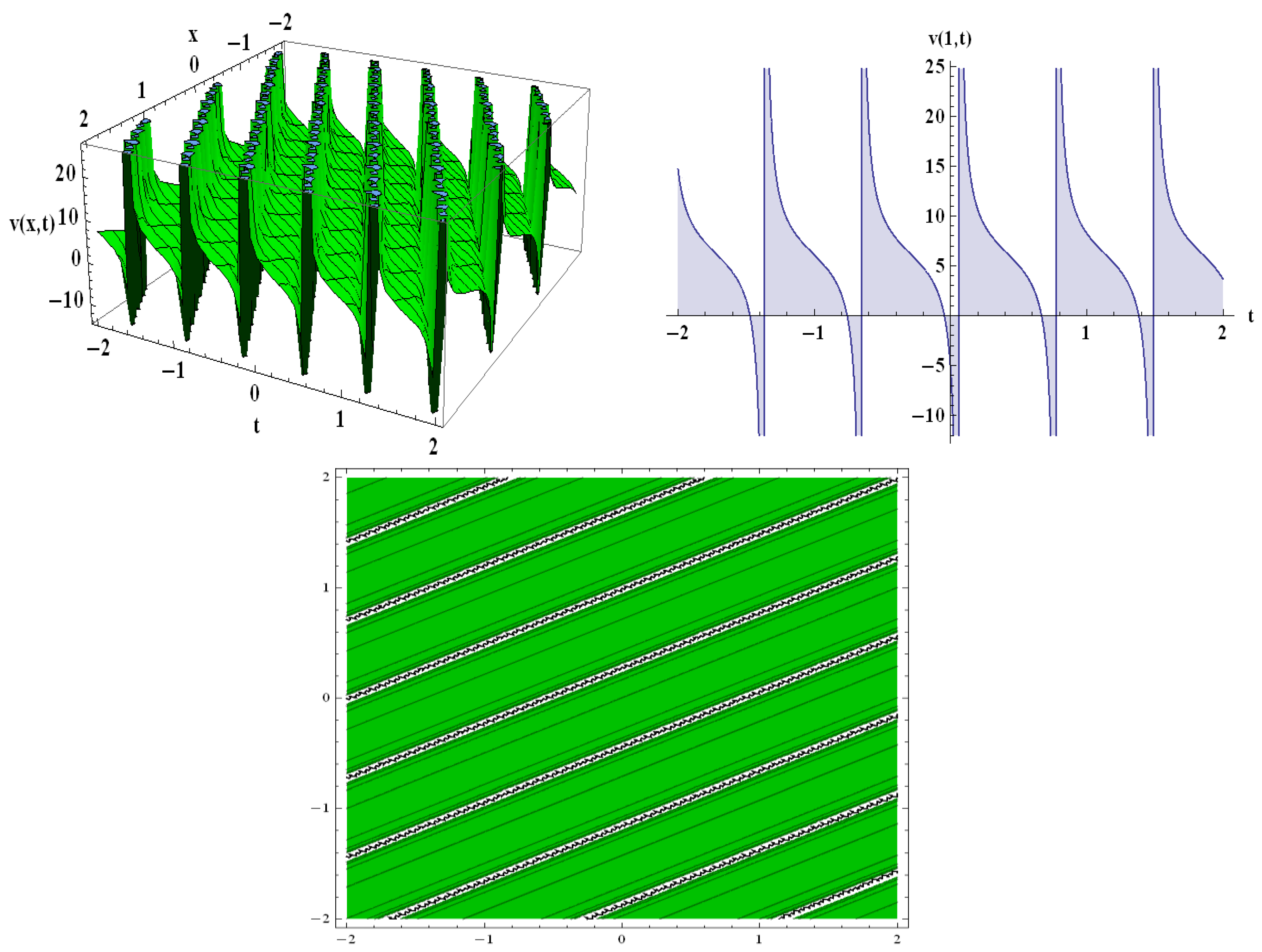
The many types of graphs are created using the wave solution. When the free parameters associated with the solution are altered, the shape of the traveling wave changes. From the Heimburg model equation, we acquire the number of exact solutions along with unknown parameters.

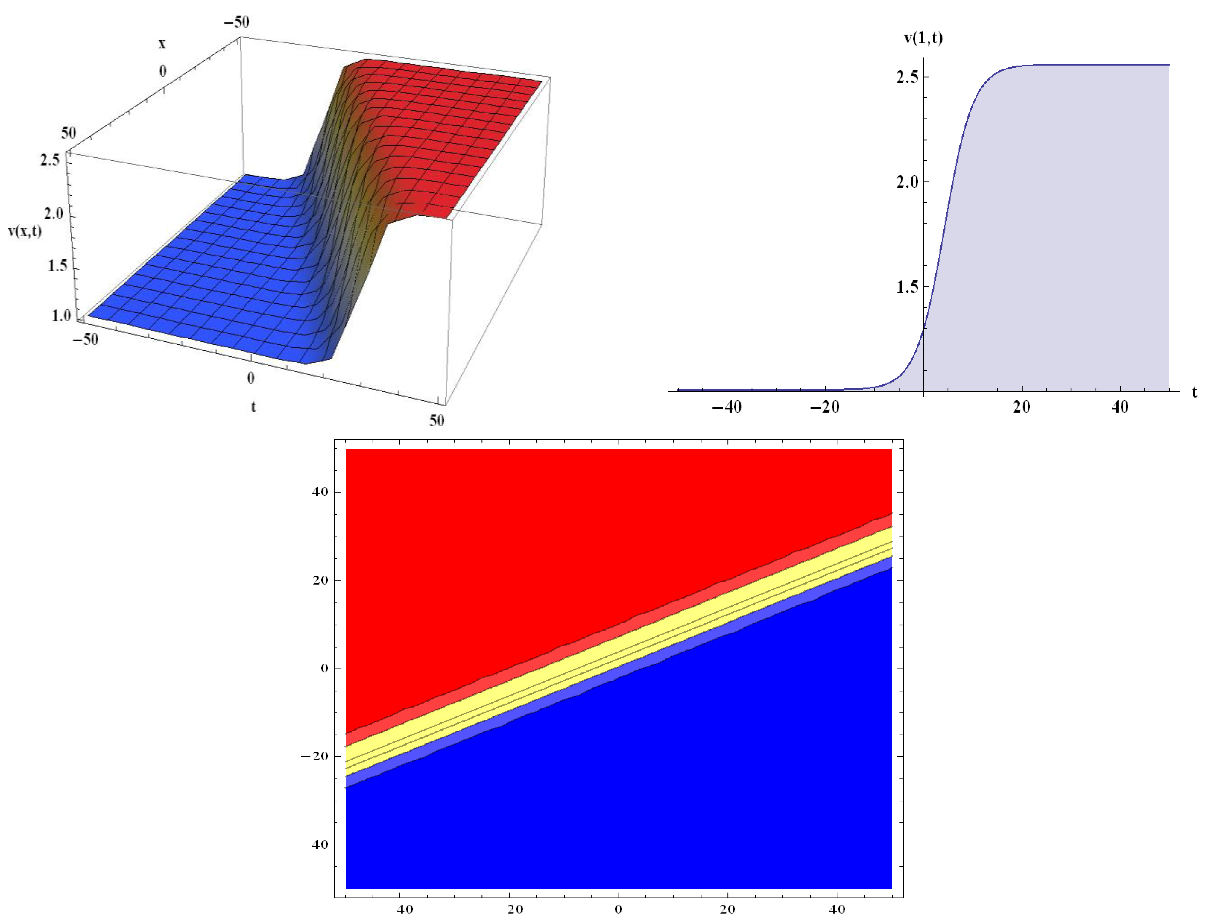
The attained solutions (20) and (22) involve the parameters ${\alpha }_1,{\beta }_1,\mu ,\omega ,\mathrm{P},$ and $a_1$. For the values of ${\alpha }_1=-0.9,{\beta }_1=2,\mu =1,\omega =2,P=0.8,$ and $a_1=5$, in solution (20), the kink-shaped input is regulated and permanently stabilized in the typical pulse shape along the nerve axon (Figure 1). 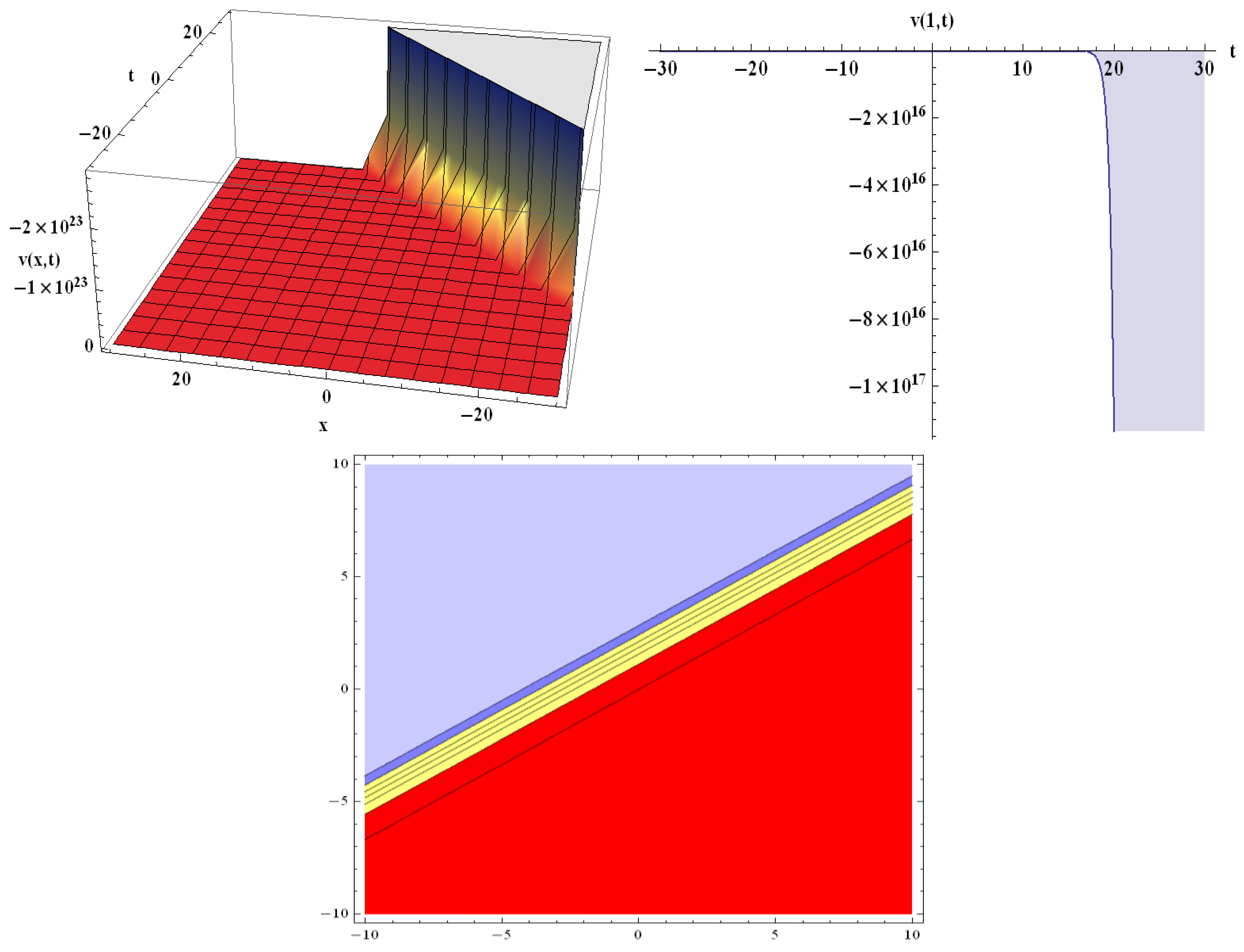Similarly, for ${\alpha }_1=-1.5,{\beta }_1=2,\mu =1,\omega =1,Q=1,$ and $a_1=1$ in solution (22), the kink-shaped input is regulated and permanently stabilized in the typical pulse shape along the nerve axon (Figure 2). 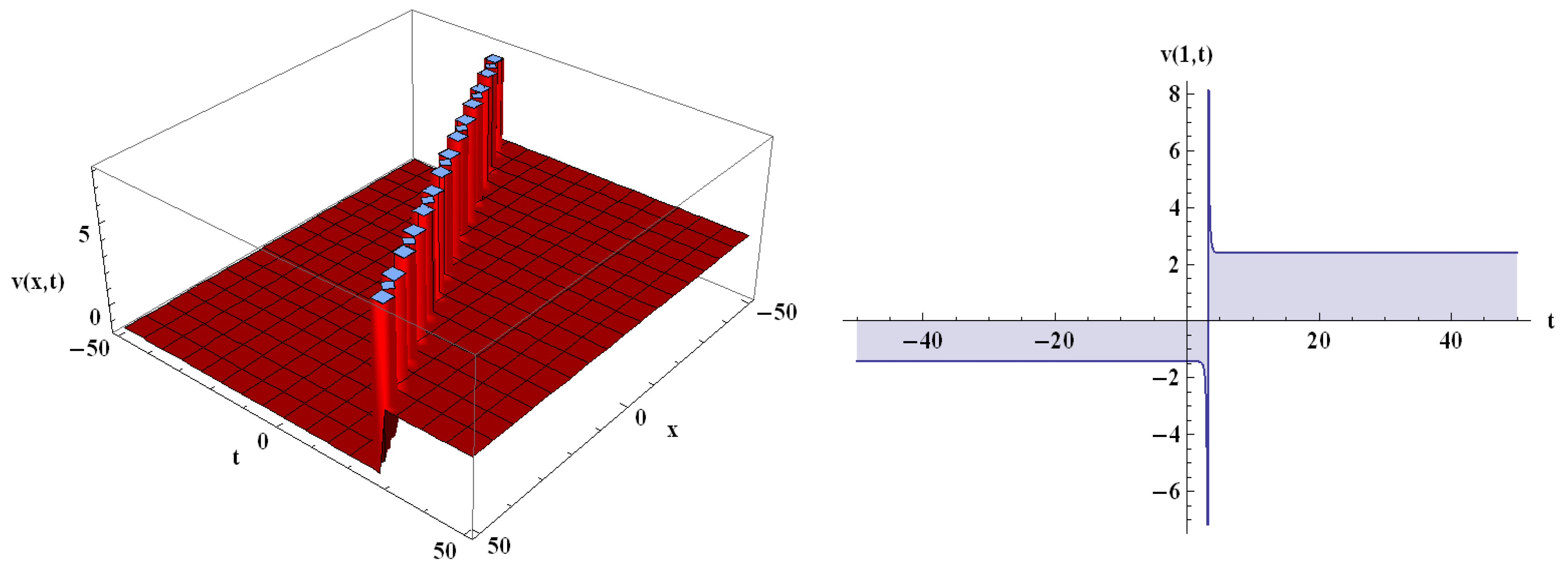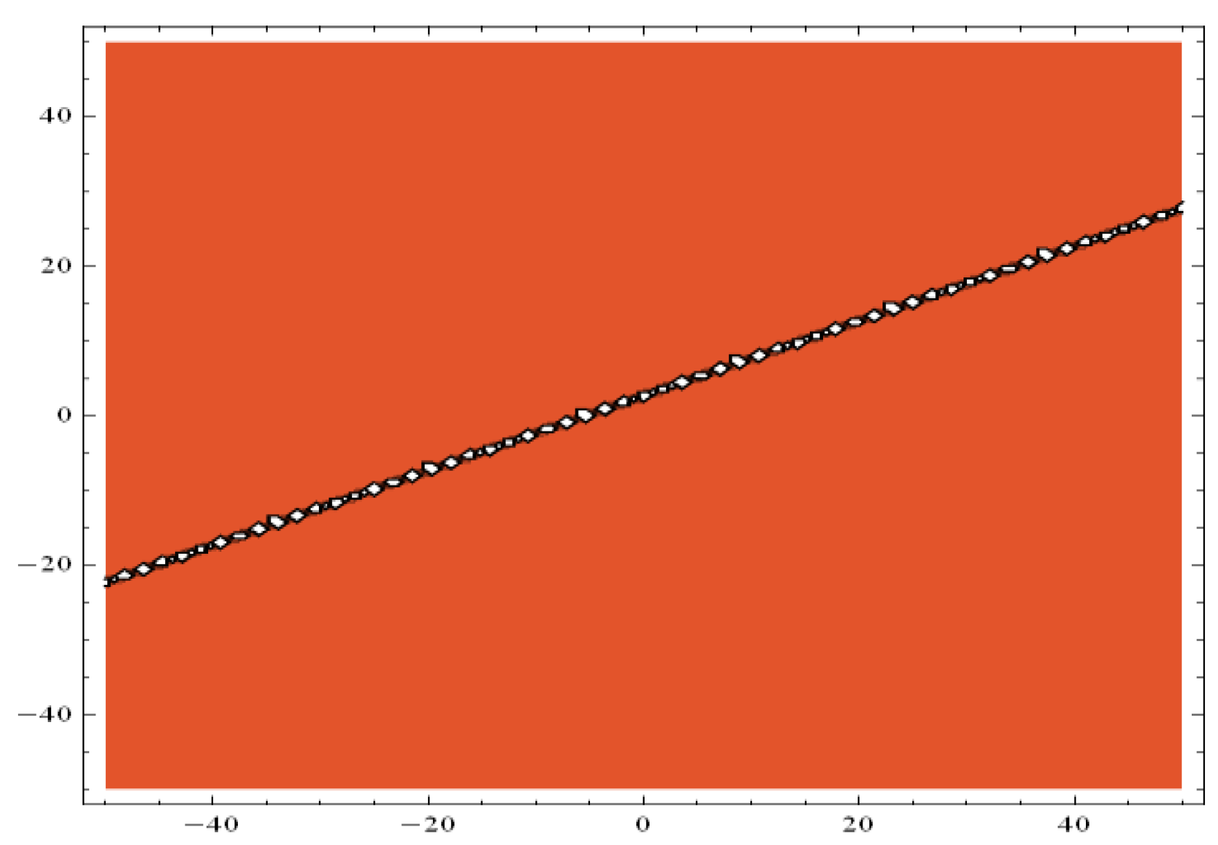For ${\alpha }_1=-0.9,{\beta }_1=2,\omega =2,P=0.8,$ and $a_1=5$, in Equation (27), the kink-shaped input is obtained (Figure 3). For ${\alpha }_1=-4,{\beta }_1=3,Q=5.6,$ and $a_1=5$, in Equation (35), the periodic-shaped input is regulated in the typical pulse shape (Figure 4). The 3D and contour plots are shown for $-50\le x,t\le 50$, and the 2D conspiracy is shown for $-50\le t\le 50$, x = 1, in Figure 1 and Figure 3; the 3D and contour plots are shown for $-30\le x,t\le 3$, and the 2D conspiracy is shown for $-30\le t\le 30$, x = 1, in Figure 2; the 3D and contour plots are shown for $-2\le x,t\le 2$, and the 2D conspiracy is shown for $-2\le t\le 2$, x = 1, in Figure 4.

The Heimburg model’s nonlinear dynamic nature is shown in Figure 1, Figure 2, Figure 3 and Figure 4. Different varieties of traveling waves are described in the inferred graphical renderings. Numerous novel exact solutions, including periodic kink, and singular-kink soliton solutions are discovered. The graphical presentation shows that the four distinct profiles constantly modulate in the form of an electromechanical pulse traveling through the axon in the nerve [27]. The findings demonstrate that the implemented technique is reliable, proficient, and dominant when it comes to analyzing different kinds of NLPDEs.

6. Conclusions

Not just in neurophysiology but also in mathematical physics, the process by which the nerve impulse is generated and propagated across the axon has been a critical challenge. We discovered the exact traveling wave solutions of the Heimburg model of neuroscience which is one of the most intriguing topics in modern bio-physics since the nerve is the foundation of life. The exp$\left(-\phi \left(\xi \right)\right)$-expansion method was utilized to analyze the Heimburg model in this research article. Traveling wave solutions were explored using the above-mentioned model. This method yields traveling wave solutions with arbitrary parameters expressed as kink, singular-kink, and periodic-wave solutions. The graphical presentation shows that the four distinct profiles constantly modulate into the pulse pattern as they travel through the axon. It is worth noting that the findings of this study are revealed for the first time, in comparison to earlier investigations. The accuracy of the results was tested using Maple 18 and putting the obtained findings into the original equation. The solutions provided are novel, distinctive, and practical and might be essential in the fields of medicine and biosciences. In other words, the analytical expression of solitary solutions may be useful for the precise determination of the control pulse’s magnitude. Additional research is required on the fascinating challenge of wave propagation in biomembranes. A thorough analysis of the dissipative effects and coupling with the action potential will be discussed in the next work.

References

- Miah, M.M.; Seadawy, A.R.; Ali, H.M.S.; Akbar, M.A. Abundant closed form wave solutions to some nonlinear evolution equations in mathematical physics. J. Ocean Eng. Sci. 2020, 5, 269–278. [Google Scholar] [CrossRef]
- Barman, H.K.; Seadawy, A.R.; Akbar, M.A.; Baleanu, D. Competent closed form soliton solutions to the Riemann wave equation and the Novikov-Veselov equation. Results Phys. 2020, 17, 103131. [Google Scholar] [CrossRef]
- Akbar, M.A.; Akinyemi, L.; Yao, S.-W.; Jhangeer, A.; Rezazadeh, H.; Khater, M.M.; Ahmad, H.; Inc, M. Soliton solutions to the Boussinesq equation through sine-Gordon method and Kudryashov method. Results Phys. 2021, 25, 104228. [Google Scholar] [CrossRef]
- Younis, M.; Seadawy, A.R.; Baber, M.; Husain, S.; Iqbal, M.; Rizvi, S.R.; Baleanu, D. Analytical optical soliton solutions of the Schrödinger-Poisson dynamical system. Results Phys. 2021, 27, 104369. [Google Scholar] [CrossRef]
- Akbar, M.A.; Kayum, M.A.; Osman, M.S.; Abdel-Aty, A.H.; Eleuch, H. Analysis of voltage and current flow of electrical transmission lines through mZK equation. Results Phys. 2021, 20, 103696. [Google Scholar] [CrossRef]
- Shah, N.A.; El-Zahar, E.R.; Chung, J.D. Fractional Analysis of Coupled Burgers Equations within Yang Caputo-Fabrizio Operator. J. Funct. Spaces 2022, 2022, 6231921. [Google Scholar] [CrossRef]
- Chang, Y.F. Neural synergetics, lorenz model of brain, soliton-chaos double solutions and physical neurobiology. NeuroQuantology 2013, 11, 56–62. [Google Scholar] [CrossRef][Green Version]
- Shah, N.A.; Hamed, Y.S.; Abualnaja, K.M.; Chung, J.-D.; Shah, R.; Khan, A. A Comparative Analysis of Fractional-Order Kaup–Kupershmidt Equation within Different Operators. Symmetry 2022, 14, 986. [Google Scholar] [CrossRef]
- Alquran, M.; Krishnan, E.V. Applications of sine-gordon expansion method for a reliable treatment of some nonlinear wave equations. Nonlinear Stud. 2016, 23, 639–649. [Google Scholar]
- Rupp, D.E.; Selker, J.S. On the use of the Boussinesq equation for interpreting recession hydrographs from sloping aquifers. Water Resour. Res. 2006, 42, 1–15. [Google Scholar] [CrossRef]
- Rani, A.; Khan, N.; Ayub, K.; Khan, M.Y.; Mahmood-Ul-Hassan, Q.; Ahmed, B.; Ashraf, M. Solitary Wave Solution of Nonlinear PDEs Arising in Mathematical Physics. Open Phys. 2019, 17, 381–389. [Google Scholar] [CrossRef]
- Zahran, E.H.M.; Khater, M.M.A. Exact Traveling Wave Solutions for the System of Shallow Water Wave Equations and Modified Liouville Equation Using Extended Jacobian Elliptic Function Expansion Method. Am. J. Comput. Math. 2014, 04, 455–463. [Google Scholar] [CrossRef][Green Version]
- Khater, M.M.A. The Modified Simple Equation Method and its Applications in Mathematical Physics and Biolog. Glob. J. Sci. Front. Res. Math. Decis. Sci. 2015, 15, 69–86. [Google Scholar]
- Wazwaz, A.M. The tanh method for traveling wave solutions of nonlinear equations. Appl. Math. Comput. 2004, 154, 713–723. [Google Scholar] [CrossRef]
- El-Wakil, S.A.; Abdou, M.A. New exact travelling wave solutions using modified extended tanh-function method. Chaos Solitons Fractals 2007, 31, 840–852. [Google Scholar] [CrossRef]
- Wazwaz, A.M. A sine-cosine method for handling nonlinear wave equations. Math. Comput. Model. 2004, 40, 499–508. [Google Scholar] [CrossRef]
- Radha, B.; Duraisamy, C. The homogeneous balance method and its applications for finding the exact solutions for nonlinear equations. J. Ambient Intell. Humaniz. Comput. 2021, 12, 6591–6597. [Google Scholar] [CrossRef]
- Ren, Y.J.; Zhang, H.Q. A generalized F-expansion method to find abundant families of Jacobi Elliptic Function solutions of the (2 + 1)-dimensional Nizhnik-Novikov-Veselov equation. Chaos Solitons Fractals 2006, 27, 959–979. [Google Scholar] [CrossRef]
- Darvishi, M.T.; Najafi, M.; Arbabi, S.; Kavitha, L. Exact propagating multi-anti-kink soliton solutions of a (3+1)-dimensional B-type Kadomtsev–Petviashvili equation. Nonlinear Dyn. 2016, 83, 1453–1462. [Google Scholar] [CrossRef]
- Khani, F.; Darvishi, M.T.; Farmany, A.; Kavitha, L. New exact solutions of coupled (2+1)-dimensional nonlinear systems of Schrödinger equations. ANZIAM J. 2011, 52, 110–121. [Google Scholar] [CrossRef]
- Ilie, M.; Biazar, J.; Ayati, Z. The first integral method for solving some conformable fractional differential equations. Opt. Quantum Electron. 2018, 50, 1–11. [Google Scholar] [CrossRef]
- He, W.; Chen, N.; Dassios, I.; Shah, N.A.; Chung, J.D. Fractional System of Korteweg-De Vries Equations via Elzaki Transform. Mathematics 2021, 9, 673. [Google Scholar] [CrossRef]
- Manafian, J.; Ilhan, O.A.; Mohammed, S.A. Forming localized waves of the nonlinearity of the dna dynamics arising in oscillator-chain of peyrard-bishop model. AIMS Math. 2020, 5, 2461–2483. [Google Scholar] [CrossRef]
- Ilhan, O.A.; Manafian, J.; Alizadeh, A.; Baskonus, H.M. New exact solutions for nematicons in liquid crystals by the tan (ϕ/ 2 ) -expansion method arising in fluid mechanics. Eur. Phys. J. Plus 2020, 135, 1–19. [Google Scholar] [CrossRef]
- Shah, N.A.; Dassios, I.; El-Zahar, E.R.; Chung, J.D. An Efficient Technique of Fractional-Order Physical Models Involving ρ-Laplace Transform. Mathematics 2022, 10, 816. [Google Scholar] [CrossRef]
- Rani, A.; Ashraf, M.; Ahmad, J.; Ul-Hassan, Q.M. Soliton solutions of the Caudrey–Dodd–Gibbon equation using three expansion methods and applications. Opt. Quantum Electron. 2022, 54, 1–19. [Google Scholar] [CrossRef]
- GAchu, F.; Kakmeni, F.M.M.; Dikande, A.M. Breathing pulses in the damped-soliton model for nerves. Phys. Rev. E 2018, 97, 1–9. [Google Scholar] [CrossRef]
- Lautrup, B.; Appali, R.; Jackson, A.D.; Heimburg, T. The stability of solitons in biomembranes and nerves. Eur. Phys. J. E. Soft Matter. 2011, 34, 1–9. [Google Scholar] [CrossRef] [PubMed]
- Peets, T.; Tamm, K.; Engelbrecht, J. On the role of nonlinearities in the Boussinesq-type wave equations. Wave Motion 2017, 71, 113–119. [Google Scholar] [CrossRef]
- Abdelrahman, M.A.E.; Zahran, E.H.M.; Khater, M.M.A. The Exp (-φ(ξ))-Expansion Method and Its Application for Solving Nonlinear Evolution Equations. Int. J. Mod. Nonlinear Theory Appl. 2015, 4, 37–47. [Google Scholar] [CrossRef]
- Pankaj, R.D.; Kumar, A.; Singh, B.; Meena, M.L. Exp (−φ(ξ)) expansion method for soliton solution of nonlinear Schrödinger system. J. Interdiscip. Math. 2022, 25, 89–97. [Google Scholar] [CrossRef]
- Hodgkin, A.L.; Huxley, A.F. Propagation of electrical signals along giant nerve fibers. Proc. R. Soc. Lond. B. Biol. Sci. 1952, 140, 177–183. [Google Scholar] [CrossRef]
- Hodgkin, A.L.; Huxley, A.F. Resting and action potentials in single nerve fibres. J. Physiol. 1945, 104, 176–195. [Google Scholar] [CrossRef]
- Hodgkin, A.L.; Huxley, A.F. Currents carried by sodium and potassium ions through the membrane of the giant axon of loligo. J. Physiol. 1952, 116, 449–472. [Google Scholar] [CrossRef]
- FitzHugh, R. Impulses and Physiological States in Theoretical Models of Nerve Membrane. Biophys. J. 1961, 1, 445–466. [Google Scholar] [CrossRef]
- Mitaku, S.; Date, T. Anomalies of nanosecond ultrasonic relaxation in the lipid bilayer transition. BBA—Biomembr. 1982, 688, 411–421. [Google Scholar] [CrossRef]
- Heimburg, T.; Jackson, A.D. On soliton propagation in biomembranes and nerves. Proc. Natl. Acad. Sci. USA 2005, 102, 9790–9795. [Google Scholar] [CrossRef]