A Roadside Unit Deployment Optimization Algorithm for Vehicles Serving as Obstacles

Abstract

As an important direction of topology management and infrastructure construction in Internet of Vehicles (IoV), the problem of roadside unit deployment has been discussed a lot. Considering the problem of communication occlusion caused by mobile vehicles, a novel multi-objective optimization problem of roadside unit deployment under the constraints of target road coverage and communication reliability is proposed in this paper. Firstly, the traffic flow model of the vehicle is introduced, and the channel model considering the occlusion of a mobile vehicle is proposed by a practical two-ray model and knife-edge diffraction model. Then, on the basis of analyzing the difficulty of the problem, an Improved Artificial Bee Colony algorithm based on Neighborhood Ranking (NR-IABC) and a Greedy Heuristic (GH) algorithm are proposed to approximately solve the problem. The NR-IABC algorithm applies the “Neighborhood Ranking” method to reduce the search domain, and then to further reduce the solution time. In order to avoid a local optimum, the sensitivity and pheromone are used as the selection strategy to replace the traditional roulette selection method in the NR-IABC algorithm. In addition, the mutual attraction between bees is involved in the neighborhood search of the following bees, and a new nectar source is generated according to the reverse learning strategy to replace the worst nectar source at the end of each iteration. Finally, results of comparative simulations based on real-life datasets show that the NR-IABC-based solution can always deploy fewer RSUs, and thus is more cost-effective compared with the GH-based solution.

1. Introduction

Internet of Vehicles (IoV) refers to the realization of a comprehensive network connection of vehicle-to-everything (V2X) with the help of a new generation of information and communication technology, such as Vehicular Ad Hoc Network (VANET). It can improve the intelligence level and autonomous driving ability of vehicles, thus improving traffic efficiency, building new formats of transportation services, and providing intelligent, comfortable, and efficient comprehensive services for users [1]. Vehicles in an IoV system need to exchange information about environments, traffic, and other vehicles in different actual application scenarios, such as smart ports, urban roads, highways, and so on [2]. Basically, an IoV system has three components: On-Board Units (OBUs) mounted on each vehicle, Roadside Units (RSUs) placed along roads, and the communication channel [3]. The OBU is used to collect and transmit information related to vehicle status, safety, etc. The RSU is fixed and deployed on the roadside for data forwarding and network maintenance. At present, a lot of research efforts related to IoV focus on the fields of network topology management and optimization, efficient routing technology and information security, etc. [4]. Among them, network topology management and optimization involve network deployment, network performance management, network fault management, etc., and are the initial work for the IoV system design and implementation. The RSU is the main infrastructure of the IoV system, and thus RSU deployment is an important direction of IoV network topology management and optimization. Specifically, the RSU deployment problem involves optimizing the number and location of RSUs under the constraints of different application scenarios and service quality to minimize the cost of IoV infrastructure. However, the RSU deployment process in real-life scenarios will face the challenges of dynamic occlusion of traffic flow, radio frequency interference, unreliable wireless channel, geographic layout, and so on [5]. Furthermore, the dynamic traffic flow consists of various metal vehicles, and thus forms intermittent occlusion of the wireless channel. Considering the universality and complexity of the occlusion caused by traffic flow, it is practical and challenging to study the RSU deployment problem under this constraint, which is rare in existing work. Moreover, the RSU deployment problem under the constraints of key service quality such as communication reliability, network coverage, communication delay [6], and throughput is a kind of multi-constrained optimization problem, and after the challenges brought by the superimposed application scenarios, the problem becomes more challenging.

Much of the literature on RSU deployment strategies ignores the impact of obstacles on communication, and assumes an ideal communication environment or even a one-dimensional scene to propose the theoretical framework of RSU deployment [7]. Based on these efforts, many scholars further consider the occlusion effect of static objects, such as buildings, trees, and large infrastructure, on communication links [8,9,10]. However, rare work considers the occlusion of mobile vehicles as obstacles [11,12]. Modeling the mobile vehicle as an obstacle is necessary, which can attenuate or even block the signal. Especially in an environment with high traffic flow, such as city roads, the distance between vehicles is relatively close, and the metal shielding of the signal is strengthened. Moreover, the changeable traffic flow aggravates the instability of communication between the RSU and mobile vehicles, and has a nonlinear correlation, which subverts the existing RSU deployment scheme based on a deterministic RSU coverage model. Therefore, we introduce the occlusion factor of dense traffic flow, propose a channel model under changeable traffic flow, and finally propose a practical RSU deployment strategy based on a controllable linearization error and heuristic algorithm to insure the network reliability in this paper. We summarize the contributions as follows:

(1) A novel channel model considering the dynamic traffic flow as the obstacles in V2X communication is proposed according to Huygens–Fresnel principle.

(2) A multi-constraint RSU deployment problem considering the traffic flow, deployment budget, and reliable communication is proposed, then its NP-hardness and rationality of discretization error are both proved, and two approximate solutions are proposed based on greedy heuristic and artificial bee colony algorithm.

(3) The defects of high randomness, local optimum, and slow convergence speed of the original ABC algorithm are improved by introducing the “Neighborhood Ranking” method, selection strategy adjustment of nectar, and optimization of position iteration.

(4) Numerical analysis based on extensive simulations verifies the accuracy, scalability, and efficiency of the two approximate solutions.

The rest of this paper is organized as follows. In Section 2, we present the related work. Section 3 introduces the relevant channel model and formulation of our problem. Next, we propose two solutions in Section 4. Analysis of the simulation results is presented in Section 5. Finally, Section 6 summarizes this work and clarifies the future research directions.

2. Related Work

Although there is no existing RSU deployment scheme for our proposed scenario, the efforts of some scholars have inspired our work. In [8], Yu et al. focused on balancing the two objectives of efficiency and coverage and establishing an RSU deployment strategy based on traffic demand. Specifically, this model optimizes both the average data delivery delay in VANETs and the number of vehicles covered by RSUs. In [13], Anbalagan et al. proposed a memetic-based RSU (M-RSU) layout algorithm to reduce communication delay and increase the coverage area between IoV devices through an optimum RSU deployment. In addition to the M-RSU algorithm, they also proposed an intrusion detection system (IDS) based on distributed machine learning (DML), which can prevent catastrophic security failures in software-defined (SD) IoV networks. In [4], Alheeti et al. proposed a new distributed roadside unit to improve the performance and connectivity of vehicles. This method is mainly based on K-means to find the best location for each roadside unit. In addition, this method supports dynamic movement, and each vehicle has long-term connectivity. In detail, the system can adapt to different locations and achieve a high connection rate with a low error rate while reducing the cost. In [14], Liang et al. studied the location optimization of an RSU for information transmission under random traffic conditions, and proposed a genetic algorithm (GA) combined with mixed integer linear programming (GA-MILP) to solve the model. In [15], Selvakumari et al. proposed Chew’s Second Delaunay Triangulation Refinement-based Optimal RSUs Deployment Scheme (CSDTR-ORDS) to ensure the maximum connectivity of vehicle to infrastructure (V2I) communication. The proposed CSDTR-ORDS is a reliable scheme for placing RSU requirements in convex maps and setting the transmission range to each individual RSU, so that each map location can certainly be covered by at least one RSU even in the case of multiple obstacles. In [9], Shi et al. tried to find better RSU deployment (RSUD) candidate locations in some grid networks with equal length streets to minimize the average reporting time of emergency messages in V2X networks. They proposed a message dissemination model for RSUD with the V2X network and a center-rule-based neighborhood search algorithm (CNSA). In [16], Guerna et al. propose a new bio-inspired RSU placement system called ant colony optimization system for RSU deployment in VANET (AC-RDV). Through graph-based modeling, a new description of RSU deployment problem is proposed, that is, maximizing intersection coverage. The number of RSU intersections that ensure the maximum network connectivity is found. In [6], Ahmed et al. studied the problem of placing RSUs on roads similar to highways, and proposed an integer linear programming model with the goal of minimizing network delay to describe the network under consideration. However, the above models regard vehicles as mutually independent dimensionless entities, which ignores the interference caused by environmental factors on V2X communication. Obviously, the impact of static or dynamic obstacles on communication reliability is inevitable in a real scene, and then these efforts are not practical.

To solve this problem, some literature further considers the effect of static obstacles on communication. In [17], Lytaev et al. are devoted to the study of radio wave propagation modeling in an urban environment. They applied the three-dimensional bi-directional parabolic equation (PE) method to specific problems for the first time. Buildings and other obstacles are modeled by impervious (fully conductive) cuboids. It can simulate the harmonic radiation source with an arbitrary pattern. In [18], Li et al. introduced the measurement and analysis of propagation channels in V2I scenarios. First, they proposed a method based on deterministic geometry. According to the environmental characteristics of roadside trees, V2I links are divided into three types. Secondly, for each link, they studied the large-scale fading effect on the V2I channel, including the path loss index and shadow component. Subsequently, they verified the empirical path loss model by using a large number of measurements and two classical channel models. Finally, they also analyzed small-scale fading effects, including the fading depth and distance-dependent Ricean K-Factor. In [19], Kang Kim et al. proposed a neural evolutionary adaptive beamforming scheme based on enhanced topology to control the radiation pattern of the antenna array, so as to mitigate the impact of shadows in urban V2V communication at intersections. In [20], Eshteiwi et al. study the performance of V2V cooperative wireless communication based on full-duplex Amplify and Forward (AF) relay over Nakagami-m fading channels. They consider independent and not necessarily identically distributed (i.n.i.d) Nakagami-m fading channels and derive new exact and asymptotic outage probabilities for exact equivalent and approximate signal-to-interference-plus-noise ratio (SINR), respectively. Furthermore, a lower bound on the symbol error rate of the considered system is derived. The results demonstrate the significant impact of the considered interference and blocking on the system performance. This highlights the importance of considering these phenomena in performance evaluation in order to assess the practical limitations of V2V cooperative wireless communication. In [21], Hoque et al. provide experimental test data and analysis to quantify the effects of relative vehicle speeds, height differences between vehicles, and internal obstacles on V2V communication range and on-side traffic reliability in urban and highway environments, and further discuss how these results can adversely affect the design parameters of safety-critical applications by considering a V2V application “Safe Traffic Advisory” on a two-lane rural highway. In [22], He et al. show the measurements and model the propagation channel, where the bus acts as both a shading object and a relay between two passenger cars. They analyzed the effects of the bus location and car separation distance on path loss, shadowing, small-scale fading, delay spread, and cross-correlation. By using the Akaike information criterion and the Kolmogorov–Smirnov test, the Nakagami distribution was found to describe the statistics of small-scale fading well. The distance dependence of path loss is analyzed and a stochastic model is established. However, the experiment only considered the impact of the school bus as an obstacle, and the shadow effect caused by the closed metal body such as a truck and trailer will be more obvious. In [23], Abbas et al. proposed a shadow fading model based on real measurements in urban and highway scenes. The measured data are divided into three categories in the study: line-of-sight (LOS), obstructed line-of-sight (OLOS) by vehicles, and non-line-of-sight (NLOS) due to buildings. When obstacles protrude into the signal path in the Fresnel zone, the deflected signals are out of phase with the direct signal, and then the direct signal can be attenuated or even blocked completely. Therefore, the channel model based on the Huygens–Fresnel principle is more practical compared with those channel models without considering the effect of deflected signal, and is involved in this paper. These efforts effectively expand the field of theory and application, but none of them can be applied to our problem in two aspects. First, we consider the moving traffic flow as a dynamic obstacle, which increases the nonlinearity of the communication channel. Second, a multi-objective optimization problem for RSU deployment constrained by dynamic obstacles, deployment budget, and communication reliability subverts the existing RSU deployment scheme based on the deterministic RSU coverage model, and the research on its problem characteristics and solutions needs to be proposed.

3. Relevant Models and Problem Formulation

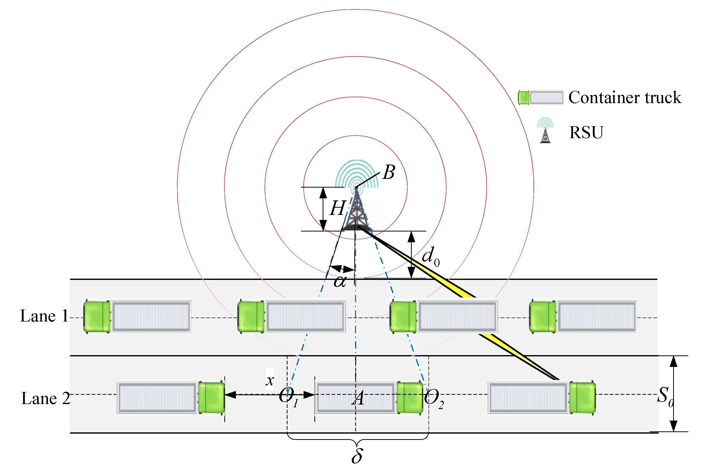
3.1. The Traffic Flow Model

Because it is difficult to accurately analyze the channel model under mixed traffic flow, the most serious occlusion of traffic flow as dynamic obstacles of wireless channels is adopted in this paper when the traffic flow is formed all by container trucks. We introduce a two-lane road scenario as shown in Figure 1, which is normal on urban city roads, smart ports, or highways. The road is busy with a large number of trucks. Furthermore, the dimension of the container truck is adopted for normalization. Because an RSU has higher transmission power and receptive sensitivity than that of an OBU, the downlink from an RSU to OBU is much more reliable than the uplink from an OBU to RSU. Therefore, when a mobile truck is covered by an RSU in this paper, the reliability of the uplink from the OBU to the RSU must meet the pre-set conditions, which means that the reliability of the uplink is used to evaluate the coverage of the OBU by the RSU in this paper.

Figure 1. Model of traffic flow under the fading channel condition.

We suppose the trucks are all driving along the middle line of the lane because the width of the lane is negligible relative to the transmission distance between the RSU and the OBU. The parameters and the variables used in the problem statement are summarized in Table 1.

Table 1. Parameters and variables used in the problem statement.

Parameters	Description
l	The length of the container truck
w	The width of the container truck
h	The height of the container truck
H	The height of the top of the RSU from the ground
$b_0$	The height of the antenna of the OBU from the ground
$s_0$	The width of the road
γ	The arrival rate of container trucks
λ	Wavelength
f	Frequency
τ	A minimum sensitivity threshold of the received signal
$D_s$	The transmitting power of the OBU
$D_r$	The received power of the RSU
Variables	Description
$d_0$	A continuous variable. The distance from the bottom of the RSU to the curb
α	A continuous variable. The angle between AB and A’B
θ	A continuous variable. The elevation angle between the antenna of the OBU and the top of the RSU
$J$	A continuous variable. The attenuation due to diffraction
$PL$	A continuous variable. The attenuation under the free-space path loss condition
$LOS{S}_{NLOS}$	A continuous variable. The total attenuation under the NLOS condition
$LOS{S}_{LOS}$	A continuous variable. The total attenuation under the LOS condition
$P_{NLOS}$	A continuous variable. The probability of the NLOS condition
$P_{LOS}$	A continuous variable. The probability of the LOS condition
$P_{nloss}^{NLOS}$	A continuous variable. Whether the signal packet is transmitted successfully under the NLOS condition
$P_{nloss}^{LOS}$	A continuous variable. Whether the signal packet is transmitted successfully under the LOS condition
$P_{nloss}$	A continuous variable. The probability of successful signal packet transmission

In the above scenario, the arrival process of vehicles to a road can be modeled as a Poisson process. Then, the probability $P\left(N=k\right)$ that there are k trucks in the road segment of length L is as follows [24]:

$$P\left(N=k\right)=\frac{\left(\gamma L{)}^k\right.}{k!}{e}^{-\lambda L}$$

(1)

where γ is the average arrival rate of the Poisson process, and is also equal to the traffic flow density.

The distance x between trucks refers to the distance from the rear of the preceding truck to the front of the following truck, as shown in Figure 1. For any two adjacent trucks, there are no other trucks in the middle. Then, the spacing probability density function (PDF) of any adjacent two trucks is given by:

$$f_x\left(x\right)=\gamma e^{-\gamma x},x\ge 0$$

(2)

3.2. Channel Model

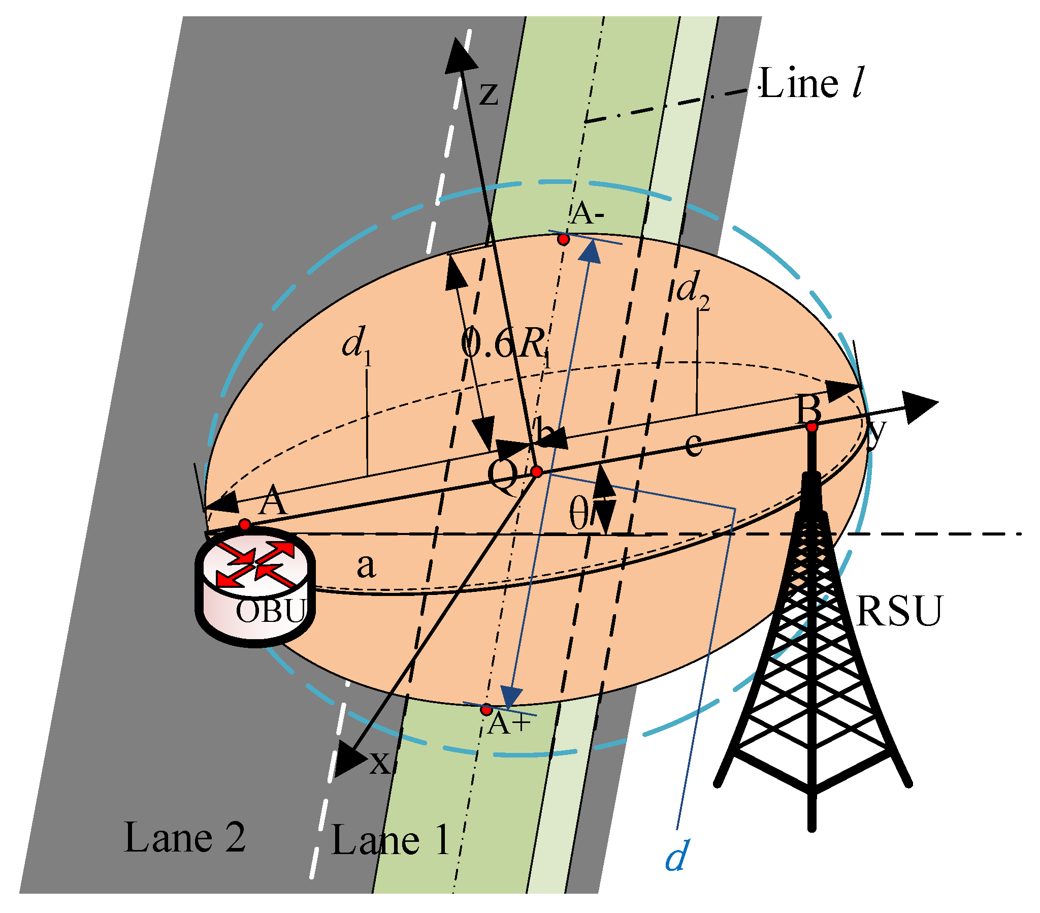
3.2.1. Preliminary Statements

There are different propagation mechanisms for the propagation model of V2I communication, usually divided into path loss (related to transmission distance), large-scale fading (including but not limited to shadows from objects significantly larger than the carrier wavelength), and small-scale fading (variations caused by multipath and/or Doppler propagation) [11]. Path loss is the expected (average) loss of received power at a certain distance. Signals from OBU can reach RSU through multiple propagation paths or multipath components (MPCs), which have different amplitudes and phases. Changes in signal amplitude due to constructive or destructive interference from different MPCs are classified as small-scale fading. Eventually, obstacles in the propagation path of one or more MPCs cause a lot of attenuation, which is an effect known as shading. Shadows can cause massive attenuation, not only on the LOS component, but also on other major MPCs. Moreover, it is reported that, in the absence of LOS, most of the power is received by single bounce reflections from physical objects [15]. Therefore, for real-world simulations and performance evaluations, it is important to describe the channel parameters as LOS and NLOS conditions, respectively, which is also adopted in this paper.

3.2.2. Probability of LOS and NLOS

Considering that the effects of static obstacles on channel propagation are additive, and this additivity will not increase the difficulty of our proposed model. Therefore, we omit the effects of static obstacles such as buildings and trees, etc., and only consider the effect of a mobile truck as an obstacle on signal propagation, and also assume that the ground is flat. When studying the propagation of radio waves between the OBU and RSU, the intermediate space can be subdivided into a cluster of concentric Fresnel ellipsoids. From the perspective of electromagnetic wave propagation, any obstacle that hinders the first Fresnel ellipsoid may affect the propagation of the signal [22]. As a practical rule, when the intrusion area of obstacles is less than 60% of the first Fresnel ellipsoid, the diffraction phenomena can be ignored, and the communication link is in a free space, which is a LOS link. Otherwise, it is an NLOS link [25]. The illustration of the attenuation effect of a mobile truck on a communication link is shown in Figure 2.

Figure 2. The illustration of the attenuation effect of a mobile truck on a communication link.

The radius of the First Fresnel ellipsoid between A (the position of the top point of OBU when the line connecting the OBU and RSU is perpendicular to the middle line of the road) and B (the top point of RSU) is given by [26]:

$$\begin{array}{c}{R}_1=550{\left[\frac{d_1{d}_2}{\left(d_1+d_2\right)f}\right]}^{\frac{1}{2}}\end{array}$$

(3)

where f is the frequency (MHz), $d_1$ and $d_2$ are the distances (km) between the A and B at the point Q where the radius (m) of the first Fresnel ellipsoid is calculated.

The calculation of the probability of a link in LOS or NLOS condition is based on the size and position of the truck. The container truck is represented as a cuboid closed metal diffracting body in our calculation for simplicity. Then, the elevation angle between A and B is θ, and its trigonometric values are:

$$\mathit{sin}\theta =\frac{H-h+1}{\sqrt{{(H+h-1)}^2+{(1.5s_0+d_0)}^2}}$$

(4)

$$\mathit{cos}\theta =\frac{1.5S_0+d_0}{\sqrt{{(H+h-1)}^2+{(1.5s_0+d_0)}^2}}$$

(5)

Suppose the position of the top of OBU at any time is A’, then the distance between A and A’ is M. The angle between AB and A’B is α, then its trigonometric values are given as follows:

$$\mathit{cos}\alpha =\frac{\frac{3}{2}{S}_0}{\sqrt{{\left(M\right)}^2+{\left(\frac{3}{2}{S}_0\right)}^2}}$$

(6)

$$\sin \alpha =\frac{M}{\sqrt{{\left(M\right)}^2+{\left(\frac{3}{2}{S}_0\right)}^2}}$$

(7)

Next, an ellipsoid E occupying the 60% of the first Fresnel ellipsoid is constructed with A’B and 0.6$R_1$ as the focal length and minor axis length, respectively, as shown by the orange ellipsoid in Figure 2. The blue dotted outline is the range of the first Fresnel ellipsoid. The parameters of the orange ellipsoid are as follows:

$$c_1=\frac{\sqrt{{\left(\frac{3}{2}{s}_0\right)}^2+{\left(H-h\right)}^2}}{2}$$

(8)

$$b_1=0.6R_1=550{\left[\frac{n{d}_1{d}_2}{\left(d_1+d_2\right)f}\right]}^{\frac{1}{2}}=550{\left[\frac{c_1{}^2}{5900\times 2c_1}\right]}^{\frac{1}{2}}$$

(9)

$$a_1=\sqrt{{\left(b_1\right)}^2+{\left(c_1\right)}^2}$$

(10)

where $a_1$, $b_1,$ and $c_1$ are the length of major axis, the length of minor axis, and the half of the focal length of the E, respectively.

Then, we assume the midpoint Q of the major axis of the E to be the origin, the minor axis of the E to be the x-axis, the major axis of the E to be the y-axis, and the z-axis to be perpendicular and upward to the xQy plane. Then, the space rectangular coordinate is established in Figure 2. The standardized equation of E is as follows:

$$\frac{x^2}{a_1{}^2}+\frac{y^2}{b_1{}^2}+\frac{z^2}{c_1{}^2}=1$$

(11)

Line l is the line passing through the geometric center of the truck. We use the distance between the intersection points of the line l and the surface of E as the length of traffic intrusion in the E. Suppose the coordinates of the two intersection points to be $A_{+}$(x+, y+, z+), $A_{-}$(x-, y-, z-), the direction vector of the line l is ($\mathit{cos}\alpha$, $\sin \alpha$, 0) and the line l passes through the point Q ($x_0$, $y_0$, $z_0$). Then, the coordinates of Q are calculated as follows:

$$\left\{\begin{array}{c}\begin{array}{c}{x}_0=0\\ y_0=\frac{d_0-0.5S_0}{2\mathit{cos}\theta \ast cos\alpha }-\left(\frac{S_0}{\frac{3}{2}{S}_0+d_0}\left(H-h-1\right)+\frac{h}{2}-1\right)\mathit{sin}\theta \end{array}\\ z_0=\left(\frac{S_0}{\frac{3}{2}{S}_0+l_0}\left(H-h-1\right)+\frac{h}{2}-1\right)\mathit{cos}\theta \end{array}\right.$$

(12)

The point direction form equation of line l is:

$$\frac{x-x_0}{cos\alpha }=\frac{y-y_0}{\mathit{sin}\alpha }=\frac{z-z_0}{0}=t$$

(13)

Substituting Equation (12) into Equation (13), we obtain:

$$\left\{\begin{array}{c}x=t·cos\alpha \hfill \\ y=t·sin\alpha +\frac{d_0-0.5S_0}{2\mathit{cos}\theta \ast cos\alpha }-\left(\frac{S_0}{1.5s_0+d_0}\left(H-h-1\right)+\frac{h}{2}-1\right)\sin \theta \hfill \\ z=\left(\frac{S_0}{1.5s_0+d_0}\left(H-h-1\right)+\frac{h}{2}-1\right)cos\theta \hfill \\ \frac{x^2}{a_1{}^2}+\frac{y^2}{b_1{}^2}+\frac{z^2}{c_1{}^2}=1\end{array}\right.$$

(14)

The solution of Equation (14) is $t_{+}$, $t_{-}$, and the length of $A_{+}{A}_{-}$ is:

$$d=\sqrt{{\left(y_{+}-y_{-}\right)}^2+{\left(x_{+}-x_{-}\right)}^2}=\left|t_{+}-t_{-}\right|$$

(15)

Combined with the truck spacing probability density function (PDF) in Equation (2), the probability of NLOS is obtained:

$$P_{\mathrm{NLOS}}={{\displaystyle \int }}_0^d\gamma e^{-\gamma x}dx$$

(16)

In addition, the probability of LOS is:

$$P_{\mathrm{LOS} }=1-P_{\mathrm{NLOS} }$$

(17)

3.2.3. Path Loss under LOS and NLOS Conditions

For the two different types of communication links LOS and NLOS, we propose a propagation model, respectively. For the condition of LOS, we use the two-ray model composed of a straight-propagating path and a ground-reflected path in the free-space path loss condition [27]. Then, the total attenuation of the signal under LOS condition is expressed as follows [28]:

$$P{L}_{}={\left(\frac{\lambda }{4\pi }\right)}^2{\left|\frac{e^{-jK{r}_d}}{r_d}+\zeta \frac{e^{-jK{r}_r}}{r_r}\right|}^2$$

(18)

where $r_d$ is the direct distance from OBU to RSU, $r_r$ is the distance reflected through the ground, λ is the wavelength, K is the number of waves, and $\zeta$ is the reflection coefficient [25]. A vertically polarized antenna model is adopted, and then the $\zeta$ can be calculated as:

$$\zeta =\frac{\mathit{sin}{\theta }_1-\frac{1}{\epsilon }\sqrt{\epsilon -{\mathit{cos}}^2{\theta }_1}}{\mathit{sin}{\theta }_1+\frac{1}{\epsilon }\sqrt{\epsilon +{\mathit{cos}}^2{\theta }_1}}$$

(19)

where ${\theta }_1$ is the angle of incidence of the reflected ray on the ground, and $\epsilon$ is the relative permittivity.

For the condition of NLOS, the attenuation is mainly due to the diffraction of electromagnetic waves. The attenuation due to diffraction depends on many factors, such as the carrier frequency, the height, material, and amount of the obstacle in the link between RSU and OBU. A verified knife-edge diffraction model is used to represent this attenuation for two reasons [12]. First, since the 5.9 GHz (5.85–5.925 GHz) frequency band or part thereof is adopted internationally as a globally or regionally harmonized dedicated frequency band for ITS by ITU-R Recommendations, f is considered to be a typical value of 5.9 GHz in this paper. Then, $\lambda$ can be calculated as approximately 0.05 m with $\lambda =c/f$, where c is the wave speed of electromagnetic ($3\times {10}^8$ m/s). Therefore, $\lambda$ is significantly smaller than the size (about 8.5 m) of the truck. Second, this verified knife-edge diffraction model involving the effect of relative locations and size of the vehicle is practical. Furthermore, the approximation of this attenuation $J$ calculated by knife-edge diffraction model can be expressed as follows [22]:

$$J=\left\{\begin{array}{c}6.9+20{log}_{10}\left[\sqrt{{(v-0.1)}^2+1}+v-0,1\right],v\ge -0.78\\ 0, v\le -0.78\end{array}\right.$$

(20)

where the calculation process of intermediate parameter v is as follows:

$$v=h\sqrt{\frac{2}{\lambda }\left(\frac{1}{r_1}+\frac{1}{r_2}\right)}$$

(21)

where h is the height of the top of the obstacle above the line connecting $T_X$ and $R_X$. $r_1$ and $r_2$ are the distances from the top of the obstacle to $T_X$ and $R_X$, respectively.

Then, the total attenuation ${\mathrm{LOSS}}_{NLOS}$ under NLOS condition is the sum of $PL$ and $J$. Furthermore, the total attenuation ${\mathrm{LOSS}}_{LOS}$ under LOS condition contains only $PL$.

$$\begin{array}{c}{\mathrm{LOSS}}_{NLOS}=PL+J\\ {\mathrm{LOSS}}_{LOS}=P\mathrm{L}\end{array}$$

(22)

3.2.4. Angular Range for Successful Transmission of Signal Packets

The received power $D_r$ of RSU under NLOS (LOS) condition can be calculated as follows:

$$\begin{array}{c}{D}_r=D_s-{\mathrm{LOSS}}_{NLOS}\\ D_r=D_s-{\mathrm{LOSS}}_{LOS}\end{array}$$

(23)

where $D_S$ is the transmitting power of OBU.

As the transmission distance and the occlusion ratio increase, the probability of successful transmission decreases. Therefore, only vehicles in a specific area may receive messages successfully from the deployed RSU. Specifically, this specific area is named as the coverage area of the RSU. It should be pointed out that the coverage area of an RSU is different from the transmission area of the RSU, and the transmission area of the RSU is a circular area limited by its transmission distance in the free-space path loss condition.

To calculate the service area of an RSU, a minimum sensitivity threshold τ of the received signal strength is introduced based on the proof in [12]. Then, the binary parameter $P_{ }{}_{\mathrm{nloss}}^{\mathrm{NLOS}}$ ($P_{ }{}_{\mathrm{nloss}}^{\mathrm{LOS}}$) for the transmission under the NLOS (LOS) condition can be calculated as follows:

$$\begin{array}{c}{P}_{ }{}_{\mathrm{nloss}}^{\mathrm{NLOS}}=\left\{\begin{array}{c}0,{\mathrm{LOSS}}_{NLOS}>D_s-\tau \\ 1,{\mathrm{LOSS}}_{NLOS}\le D_s-\tau \end{array}\right.\\ P_{ }{}_{\mathrm{nloss}}^{\mathrm{LOS}}=\left\{\begin{array}{c}0,{\mathrm{LOSS}}_{LOS}>D_s-\tau \\ 1,{\mathrm{LOSS}}_{LOS}\le D_s-\tau \end{array}\right.\end{array}$$

(24)

Because the curve of $LOS{S}_{NLOS}\left(LOS{S}_{LOS}\right)$ exhibits discrete, non-linear, fluctuating rising distributions with increasing angle, in order to calculate $P_{nloss}^{NLOS}(P_{nloss}^{LOS})$, we find the angle value ${\alpha }_1$ corresponding to the point where the total attenuation $LOS{S}_{NLOS}\left(LOS{S}_{LOS}\right)$ is closest to $(D_s-\tau )$ dBm in the attenuation curve. So, when $\alpha \in \left[0,{\alpha }_1\right)$, $P_{nloss}^{NLOS}(P_{nloss}^{LOS})=1$, otherwise, $P_{nloss}^{NLOS}(P_{nloss}^{LOS})=0$. Then, the total probability of successful packet transmission $P_{nloss}$ is calculated as follows:

$$P_{nloss}=P_{\mathrm{NLOS}}·P_{\mathrm{nloss}}^{\mathrm{NLOS}}+P_{\mathrm{LOS}}·P_{\mathrm{nloss}}^{\mathrm{LOS}}$$

(25)

As a general rule in signal propagation, when the signal packet loss rate exceeds a limiting value, the signal becomes useless [17]. Therefore, a reliability lower bound σ is introduced to constrain $P_{nloss}\left( P_{nloss}\ge \sigma \right)$. When $P_{nloss}\ge \sigma$, its value is supposed to be 1, and the rest of the values are set to be 0.

According to Equations (2), (14) and (24), the calculation of $P_{nloss}$ highly depends on the value of γ, α, $D_s$, and $d_0$. Specifically, the $P_{nloss}$ decreases with the growth of γ, α, and $d_0$, and it increases with the growth of $D_s$. Furthermore, γ, α, and $D_s$ are the preset parameter in the practice deployment, $d_0$ depends on the location of RSU and is the solution variable for the subsequent optimization problem. Therefore, the angular range that an RSU can successfully cover can be solved when the γ, $D_s$, and $d_0$ are given, and the solution process is as follows: find ${\alpha }_1$ based on Equation (25), and $P_{nloss}=1$ holds when $0\le \alpha \le {\alpha }_2$, and then the angular range that an RSU can successfully cover is $\left[0,{\alpha }_2\right],{\alpha }_2\in [0,\frac{\pi }{2})$, when γ, $D_s$, and $d_0$ are fixed.

3.3. Discretization Method and Error Analysis of Coverage Area

In order to cover the whole road, the main factor is that the candidate positions for trucks in the target coverage area are infinite, making the deployment of the RSU tricky. Obviously, the number of candidate positions is infinite (i.e., the solution space of the problem is infinite, leading to very high computational complexity). Furthermore, the proposed channel model increases the nonlinearity of the objective function in the above problem. As proved in [29], the one-dimensional RSU deployment problem is NP-hard. Therefore, as an extended problem of [29], we discretize the road to approximately solve the problem. The discretization strategy is as follows: from one side of the road, each road of length δ is discretized as one segment, and the last segment is still discretized as one segment when its length is less than δ, and the central point (CP) of a segment is used to represents the whole segment (the proof will be given in Section 4.1).

After discretization, the probability of successful packet transmission at CP represents that of each point within a segment. However, this representation will cause a discretization error μ:

$$\mu =\frac{Max\left(\Delta P_{\mathrm{nloss} }\right)}{P_{\mathrm{nloss} }^{CP}}$$

(26)

where $P_{nloss}^{CP}$ is the probability of successful packet transmission at CP, the $Max(\Delta P_{nloss})$ is the maximum $\Delta P_{nloss}=P_{nloss}^{pi}-P_{nloss}^{CP}$, $P_{nloss}^{pi}$ is the probability of successful packet transmission at any point pi, and pi belongs to a segment.

According to Equations (14), (16) and (26), μ tends to be a maximum within a unit step increment when $\alpha =0^{\circ }$, and it will be further affected by the value of $d_0$. As shown in Figure 1, the CP of segment O1-O2 is point A. Normally, $\mu \le ϵ$ holds, and the maximum segment length ${\delta }_{\max }$ can be calculated when $\mu =ϵ$, and ϵ is an empirical numerical value in actual working conditions. Then, the transmission success rate $P_{nloss}$ under NLOS condition is analyzed:

$$P_{nloss}=P_{\mathrm{NLOS}}·P_{\mathrm{nloss}}^{\mathrm{NLOS}}$$

(27)

$P_{nloss}=P_{\mathrm{NLOS} }$ holds when $P_{ }{}_{\mathrm{nloss}}^{\mathrm{NLOS}}=1$. According to the geometric relationship, α can be calculated as:

$$\alpha =actan\left(\frac{\delta }{1.5s_0+d_0}\right)$$

(28)

According to Equation (16), $d=d^{\prime }$ holds when OBU is at A, the probability of NLOS is as follows:

$$P_{NLOS}^{\prime }={{\displaystyle \int }}_0^{d^{\prime }}{f}_x\left(x\right)dx=1-e^{-\gamma d^{\prime }}$$

(29)

When OBU is at O1, $d=d^{″}$ holds when OBU is at O1, the probability of NLOS is as follows:

$$P_{NLOS }^{″}= {{\displaystyle \int }}_0^{d^{″}}{f}_x\left(x\right)dx=1-e^{-\gamma d^{″}}$$

(30)

Therefore, the error is:

$$\mu =\frac{P_{\mathrm{NLOS} }^{″}-P_{\mathrm{NLOS} }^{\prime }}{P_{\mathrm{NLOS} }^{\prime }}=\frac{1-e^{-\gamma \left(d^{″}-d^{\prime }\right)}}{e^{-\gamma d^{\prime }}-1}$$

(31)

According to Equations (16) and (26), when $d_0$ is 0, the change in δ per unit length has the most serious impact on μ. Therefore, we discuss the influence of δ on the error $\mu$ when $d_0=0$ satisfies. For example, when $ϵ=0.05$, ${\delta }_{\max }\approx 2.4$. Therefore, when $0\le \delta \le 2.4$, μ is within a reasonable range.

3.4. Problem Formulation

Based on the above models, we formulate the RSU deployment (RSUD) as a multi-objective optimization problem with the constraints of minimum deployment budget, coverage of target area, and communication reliability, as follows:

$$\begin{array}{c}minN\\ \mathrm{subject} \mathrm{to}: {\displaystyle {\displaystyle \sum }_{i=1}^N}{p}_i=1\\ P_{nloss}^s\ge \sigma ,\forall s\in P\end{array}$$

(32)

where N represents the total number of the deployed RSUs, $C_i$ represents the number of covered segments by ith deployed RSU, $p_i$ represents the coverage ratio for each RSU, and $p_i=\frac{C_i}{\left|P\right|}$, P represents the set of all segments, s is a segment, and $s\in P$.

3.5. Hardness Analysis

The proposed RSUD problem is similar to the well-known Geometric Set Cover (GSC) problem [29]. First, we assume that each RSU can cover an angle of (0, 2π) within the target area. Therefore, the problem becomes a conventional linear disc covering problem, that is, the GSC problem. Furthermore, the set of all CP is the coverage target. The GSC problem is a special case of the set covering the (GC) problem, which is known as NP-Hard. As a result, the proposed RSUD problem is NP-Hard.

4. Solutions

In this section, we firstly propose two approximate solutions to the above problem, namely the Greedy Heuristic (GH) algorithm and Improved Artificial Bee Colony algorithm based on Neighborhood Ranking (NR-IABC). Next, the algorithm details and time complexities of these two solutions are presented.

4.1. Search Domain Adjustment-Neighborhood Ranking

According to Equations (16) and (25), the successful signal packet transmission decreases with the growth of the distance between the RSU and target point or segment. Therefore, a suitable neighborhood ranking domain for each CP should be found to deploy an RSU.

We use two variables to describe the coverage of a road segment by an RSU: one is the angular range for successful transmission of signal packets, and the other is the conservative coverage radius R. Furthermore, when a CP point of any road segment is within the angular range for successful transmission of signal packets, and the Euclidean distance between the CP and the RSU is less than or equal to R, we consider the CP to be covered by this RSU. First, $R_0$ is the minimum value of the maximum reliable coverage distance of an RSU at any angle α (α∈[0, α2]). Specifically, for a fixed RSU, $d_0$ is a fixed value, and then the maximum reliable coverage distance increases with the growth of α according to Equations (14) and (16). Therefore, $R_0$ equals the maximum reliable coverage distance when α = 0. As shown in Figure 1, to ensure the coverage of a segment (O1-O2) by an RSU, an intuitive method is to ensure the coverage of the furthest point O1(O2) by the RSU, which means that the distance between O1(O2) and the RSU is $R_0$. Under this condition, the distance between the RSU and the CP of O1-O2 is the conservative coverage radius R, and R is calculated as:

$$R=\sqrt{R_0^2-{\left(\frac{\delta }{2}\right)}^2}$$

(33)

As a result, a circle with a CP as the center and 2R as the radius is built, which is the neighborhood ranking domain for each CP, which can ensure that any adjacent CPs (within the same neighborhood ranking domain) share one RSU to save the number of deployed RSUs. Next, all CPs are ranked in a descending order according to the number of neighboring other CPs within the neighborhood ranking domain. Finally, the two approximate algorithms can be solved based on the descending order.

4.2. Greedy Heuristic Solution

In the GH solution, the RSU deployment area is discretized into square grids with length g. It should be pointed out that the accuracy and time complexity of the GH solution will increase with the reduction in g [30]. The granularity mainly affects the accuracy and time of the calculation. Z represents the set of all discrete RSU candidate positions in the deployment area. Furthermore, the center point of each grid is used to represent the position of the candidate RSU. We assume that there is only one truck in each grid at the same time.

The process of the GH solution is shown in Algorithm 1: First, discretize target coverage roads and RSU deployment areas into grids. Second, sort all CPs of road segments in descending order according to the number of neighbor CPs within the neighborhood ranking domain. We assume that the circle with R as the radius and CP as the center is the RSU search domain of the CP. Then, the RSU for each CP should be deployed within the RSU search domain of that CP, and the RSU for CP with the largest number of neighbor CPs should be preferentially deployed. Before deploying a new RSU, each CP should be checked whether it has been covered by the deployed RSUs. Then, when deploying a new RSU, the location with the highest coverage $p_i$ within the search domain should be chosen. The deployment process will be terminated until all CPs are covered. The pseudocode of the GH algorithm is shown in Algorithm 1:

Algorithm 1 GH algorithm

Input: CPs, Z Output: The deployment set W of RSUs 1: Calculate R; 2: Sort all CPs in descending order according to the number of CPs within the neighborhood ranking domain; 3:  for i = 1:$\left|CPs\right|$ do 4:    Find uncovered CPs; 5:    for j = 1:$Z_i$ 6:      select a candidate RSU location r∈$Z_i$ that maximizes $p_i$; 7:      W←W∪{r}; 8:    end for 9:  end for 10: return W

For the GH algorithm, the time complexity of discretization is $O\left({\left|CPs\right|}^2+{\left|Z\right|}^2\right)$ and the complexity of neighborhood ranking of all road segments and deployment area is $O\left({\left|CPs\right|}^2\right)$. Then, in each deployment of RSU, the number of candidate locations needs to be checked $\left|Z_i\right|$ times to calculate the maximum $p_i$, and $\left|Z_i\right|\le \left|Z\right|$, and the time complexity to calculate $p_i$ is $O\left({\left|CPs\right|}^2\right)$. Therefore, the time complexity to deploy RSUs for all CPs is $O\left({\left|CPs\right|}^2\cdot \left|Z\right|\right)$. Finally, the time complexity of Algorithm 1 is:

$$O=O\left({\left|CPs\right|}^2+{\left|Z\right|}^2\right)+O\left({\left|CPs\right|}^2\right)+O\left({\left|CPs\right|}^2\cdot \left|Z\right|\right)=O\left({\left|CPs\right|}^2+{\left|Z\right|}^2\right)+O\left({\left|CPs\right|}^2\cdot \left|Z\right|\right)$$

(34)

According to Equation (34), the time complexity of the GH algorithm highly depends on the discretization granularity g and δ, when the problem scenarios are fixed.

4.3. Improved Artificial Bee Colony Algorithm based on the Neighborhood Ranking Solution

When inappropriate discretization granularity is used, the solution of GH tends to a local optimum. The swarm intelligence optimization algorithm such as the artificial bee colony (ABC) algorithm mainly seeks the optimal solution by imitating the intelligent honey-collecting activities of the bee colony, through the role transformation and cooperation principles between bees. The traditional ABC algorithm has some disadvantages: first, too large a search domain results in a long solution time. Second, it has strong randomness due to the roulette selection method and it falls easily into a local optimum. Third, the influence of all leading bees on the process of the following bee’s neighborhood search is not considered. Fourth, the worst solution produced at the end of each generation leads to slower convergence during iterations. Therefore, this paper makes the following improvements from four aspects—search domain adjustment (explained in Section 4.1), selecting methods, introducing mutual gravitational coefficients, and replacement of the worst honey source. Therefore, we propose the NR-IABC algorithm, which has good generalization performance:

(1) The adjustment of the select method.

The roulette selection method in the traditional ABC algorithm will reduce the diversity of the population and cause the phenomenon of excessive convergence. According to [31], we consider using the combination of sensitivity and pheromone to carry out the process of selecting nectar sources for the following bees. The process can be divided into the following four steps:

Step 1: Calculate the fitness value of SN nectar sources $fi{t}_i, i=1,2,\dots ,SN$

Step 2: Calculate the pheromone of the nectar source $O\left(i\right)$:

$$O\left(i\right)=\left\{\begin{array}{cc}\frac{fi{t}_i-fi{t}_{min}}{fi{t}_{max}-fi{t}_{min}},\hfill & fi{t}_{max}\ne fi{t}_{min};\hfill \\ 0,\hfill & \mathrm{others}\hfill \end{array}\right.$$

(35)

Step 3: Randomly generate the sensitivity of the ith following bee $S\left(i\right)\sim U\left(0,1\right)$.

Step 4: If the sensitivity $S\left(i\right)$ of the ith following bee is less than the pheromone $O\left(i\right)$ of the ith nectar source, perform a neighborhood search to generate a new nectar source (new solution) $v_i$. Then judge its fitness value: if it is better, replace the original nectar with the new nectar; if $S\left(i\right)>O\left(i\right)$, the following bee follows the lead bee, and the position of the nectar source remains unchanged.

(2) The introduction of the mutual gravitation.

In the ABC algorithm, the following bee can only randomly select a nectar source found by the lead bee to complete the neighborhood search, thus narrowing the search area of the follower bee and leading to a local optimum. Therefore, considering the introduction of the gravitational force [32] between the follower bees and the leading bees, the following interaction strategy is given. Newton’s formula for universal gravitation is as follows:

$$F_{12}=G\frac{m_1{m}_2}{r_{21}^2}{\overrightarrow{r}}_{21}$$

(36)

where $F_{12}$ represents the gravitational force between two objects, $G$ is the gravitational constant, $m_1$ and $m_2$ are the mass of the two objects, $r_{21}$ represents the distance between two objects, and ${\overrightarrow{r}}_{21}$ represents the following unit vector.

$${\overrightarrow{r}}_{21}=\frac{r_2-r_1}{\left|r_2-r_1\right|}$$

(37)

$m_1$ is replaced by the fitness value $F\left(x_i\right)$ of the ith leading honey source, $m_2$ is replaced by the fitness value $F\left(x_k\right)$ of the kth leading honey source. Let there be a total of SN leading bees, that is, $k=1,2,\dots ,SN,$ and $k\ne i$.

$$F_{ik}=G\frac{F\left(x_i\right)·F\left(x_k\right)}{{\left(x_k-x_i\right)}^2}·\frac{x_k-x_i}{\left|x_k-x_i\right|}$$

(38)

$$F_{i{k}_j}=G\frac{F\left(x_i\right)·F\left(x_k\right)}{{\left(x_{kj}-x_{ij}\right)}^2}·\frac{x_{kj}-x_{ij}}{\left|x_{kj}-x_{ij}\right|}$$

(39)

Then, the formula in the algorithm that follows the honey source update becomes:

$$v_{ij}=x_{ij}+F_{i{k}_j}\left(x_{ij}-x_{kj}\right)$$

(40)

To ensure $F_{iR}\in \left[0,1\right]$, $F_{iR}$ can be standardized to ${\tilde{F}}_{ik}$:

$$Total\left(F_{ik}\right)= {\displaystyle \sum }_{\begin{array}{c}k=1\\ k\ne i\end{array}}^{SN}\left[G\frac{F\left(x_i\right)·F\left(x_k\right)}{{\left(x_k-x_i\right)}^2}\right]$$

(41)

$${\tilde{F}}_{ik}=\frac{\left|G\frac{F\left(x_i\right)·F\left(x_k\right)}{{\left(x_k-x_i\right)}^2}·\frac{x_k-x_i}{\left|x_k-x_i\right|}\right|}{Total\left(F_{ik}\right)}$$

(42)

The leading and following bees update the nectar source as follows:

$$v_{ij}=x_{ij}+R_{ij}\left(x_{ij}-x_{kj}\right)$$

(43)

Substitute Equation (42) to Equation (43), and we obtain:

$$v_{ij}=x_{ij}+ {\displaystyle \sum }_{\begin{array}{c}k=1\\ k\ne i\end{array}}^{SN}{\tilde{F}}_{i{k}_j}\left(x_{ij}-x_{kj}\right)$$

(44)

The following bees generate a new nectar source when neighborhood searching according to Equation (44).

(3) Replacement of the worst honey source.

Because the ABC algorithm tends to rely on the worst nectar source of the current generation to reduce the new nectar source according to Equations (43) and (44), which is not conducive to obtaining the optimal result. Correspondingly, it also has a negative influence on the convergence speed of the algorithm. Therefore, we consider replacing the worst nectar source with the newly generated nectar source [33], which has mathematically shown that the reverse learning strategy is a better estimate of the original candidate solution. This method can be expressed as follows:

After each iteration, the position of the worst honey source is denoted as $x_i$, and represents the position of the newly generated honey source to $x_i^{\prime }$, $x_{ij}$ is the jth component of $x_i$, and the jth component $x_{ij}^{\prime }$ of $x_i^{\prime }$ is calculated as follows:

$$x_{ij}^{\prime }=x_{i{j}_L}+x_{i{j}_U}-rand\left(0,1\right)·x_{ij}$$

(45)

where $x_{i{j}_L}$ represents lower bound of the jth component of $x_i, x_{i{j}_U}$ represents upper bound of the jth component of $x_i$, that is, $x_{i{j}_L}\le x_{ij}\le x_{i{j}_U}$, $j\in \left\{1,2,\dots ,d\right\}$. If $x_{ij}^{\prime }>x_{i{j}_U}, x_{ij}^{\prime }=x_{i{j}_U}$; if $x_{ij}^{\prime }<x_{i{j}_L}, x_{ij}^{\prime }=x_{i{j}_L}$.

For each component of the worst nectar source, Equation (45) is used to update the new nectar source. If the new nectar source is better, it is used to replace the original nectar source.

The process of the NR-IABC solution is shown in Algorithm 2: First, discretize the target coverage roads and RSU deployment areas into grids. Second, sort all CPs of road segments in descending order according to the number of neighbor CPs within the neighborhood ranking domain. Before deploying a new RSU, each CP should be checked whether it has been covered by the deployed RSUs. Then, we preferentially use the NR-IABC algorithm to deploy a new RSU within the search domain of the CP that has the largest number of neighbor CPs at each iteration. This avoids low coverage with bees located near the center of the area, allowing each RSU to maximize its coverage. The deployment process will be terminated until all CPs are covered.

The process of the NR-IABC algorithm is as follows:

Step 1: Algorithm initialization. Including the size of initialized population, control parameter limit, the maximum iteration number MaxIt, training set trail is initialized to zero vector, the maximum element of trail TR, and randomly generate SN initial solutions $x_i,i=1,2,\dots ,SN$, according to Equation (46):

$$x_i^j=x_{min}^j+rand\left(0,1\right)\left(x_{max}^j-x_{min}^j\right)$$

(46)

Next, calculate the fitness value of function Fitness( ) for each solution (Fitness( ) is a function that calculates the proportion of covered CPs to the total CPs);

Step 2: The leading bee constructs a new solution $v_i$ according to Equation (43), and then finds its fitness value; if the fitness value of $v_i$ is better than that of $x_i$, then $x_i$ is replaced by $v_i$, so that $v_i$ is regarded as the best solution so far; otherwise, remain $x_i$, corresponding to the ith element of the trail + 1;

Step 3: Calculate all fitness values of $x_i$, and calculate the pheromone $O(i)$ of the ith nectar source according to Equation (35);

Step 4: The following bees select the nectar source by combining the sensitivity with the pheromone, and randomly generate the sensitivity of the ith follower bee with $S(i)~U(0,1)$($U(0,1)$ means the random variable follows a uniform distribution on (0, 1)). If $S(i)\le O(i)$, then a new solution $v_i$ is generated according to Equation (44). Moreover, if the fitness value of $v_i$ is better than that of $x_i$, $x_i$ is replaced by $v_i$ and the corresponding element is reset to 0; otherwise, it remains unchanged, corresponding to the ith element of the trail + 1; if $S(i)>O(i)$, then follow the lead bee, and the position of the nectar source remains unchanged, that is, keep $x_i$ unchanged;

Step 5: Observe each element of the trail, record the largest element value, and check if any solutions need to be discarded. If a solution is not updated after more than limit iterations; that is, the maximum element value is greater than limit; then, the scouting bee generates a new solution $x_i$ according to Equation (46) to replace the maximum element of the trail. Then, the corresponding component of trail is set to 0;

Step 6: Find the worst solution, and update it according to Equation (45) for each component; then, a new solution ${x_i}^{\prime }$ is obtained, and calculate its fitness value. If the fitness value of ${x_i}^{\prime }$ is better than $x_i$, replace $x_i$ with ${x_i}^{\prime }$, and set the corresponding component of trail to 0; otherwise, keep $x_i$ unchanged;

Step 7: When an iteration ends, record the best solution obtained by the search process;

Step 8: Check whether the conditions for the end of the loop are satisfied. If so, output the optimal solution; if not, jump back to step 2.

The pseudocode of the NR-IABC algorithm is shown in Algorithm 2:

Algorithm 2 NR-IABC algorithm

Input: CPs, Z Output: The deployment set W of RSUs 1: Calculate R; 2: Sort all CPs in descending order according to the number of CPs within the neighborhood ranking domain; 3: for i = 1:$\left|CPs\right|$ do 4: Find uncovered CPs; 5: While the number of iterations Ite≤MaxIt do 6:    Randomly generated initial solution $x_i\in Z$ with Equation (46); 7:    Update $x_i$ with $v_i$ constructed by Equation (43), otherwise the ith element      of trail + 1; 8:    $\mathrm{Calculate} O(i)$ with Equation (35); 9:    $S(i)~U(0,1)$; 10:      if $S(i)\le O(i)$ 11:     $\mathrm{Update} x_i$ with $v_i$ constructed by Equation (44) and the ith element of trail set to 0, otherwise the ith element of trail + 1; 12:      end if 13:      if TR > limit 14:     Update TR with a new solution $x_i$ generated by the scouting bee with         Equation (46) and the ith element of trail set to 0; 15:    end if 16:    Update the worst solution $x_i$ with ${x_i}^{\prime }$ constructed by Equation (45) and the        ith element of trail set to 0; 17:    Ite = Ite + 1; 18:    Update all $\left|CPs\right|$; 19:    W←W∪$\{x_i$}; 20: end while 21: end for 22: return W

For the NR-IABC algorithm, the time complexity of discretization is $O\left({\left|CPs\right|}^2\right)$ and the complexity of neighborhood ranking of all road segments and deployment area is $O\left({\left|CPs\right|}^2\right)$. Then, in each deployment of RSU, the deployment of all RSUs is implemented in MaxIt iterations, and all nPop bees update $M_0$ in each iteration. Furthermore, the fitness value of each bee can be calculated in $O\left(MaxIt\right)$. Finally, the update of all nectar sources in each iteration can be performed in $O\left(MaxIt\right)$. Therefore, the time complexity to deploy RSUs for all CPs is $O\left(MaxIt\cdot \left(M_0\cdot nPop\cdot MaxIt+MaxIt\right)\right)$. Finally, the time complexity of Algorithm 2 is:

$$O=O\left({\left|CPs\right|}^2\right)+O\left({\left|CPs\right|}^2\right)+O\left(MaxIt\cdot \left(M_0\cdot nPop\cdot MaxIt+MaxIt\right)\right)=O\left({\left|CPs\right|}^2\right)+O\left(M_0\cdot nPop\cdot MaxI{t}^2\right)$$

(47)

5. Numerical Results

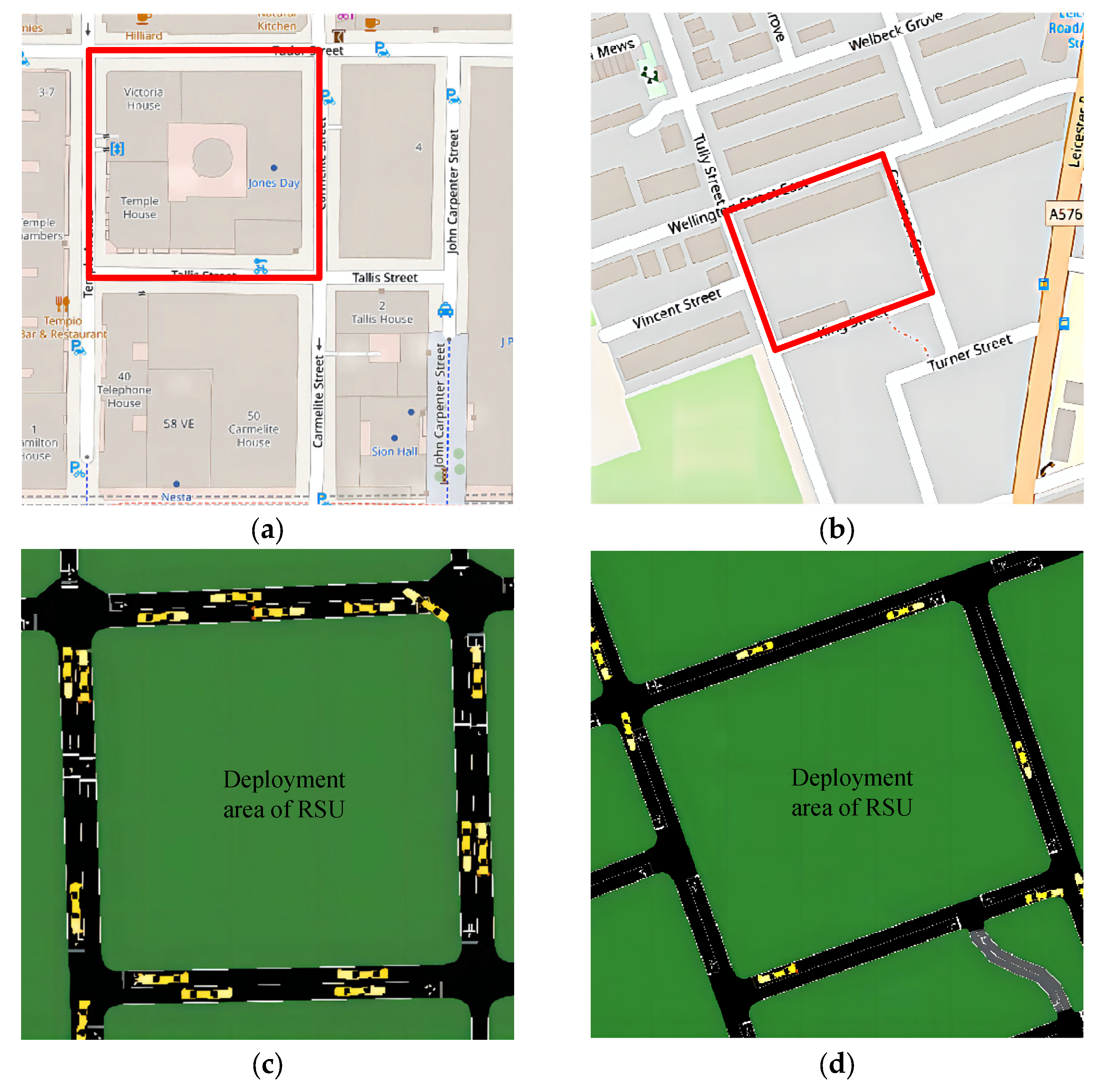
5.1. Simulation Settings

In order to determine a reasonable range for simulation parameters, we refer to real-life datasets. First, two different real-life datasets are chosen—central city in London and an industrial area in Manchester—as target locations for RSU deployments. Additionally, these two scenarios are obviously different because the central city in London has a higher traffic flow density than that in Manchester. Second, we intercept two rectangle road networks in the above scenarios, because the rectangle road network is common in a real-life road layout. OpenStreetMap is applied to provide the geometry data of the maps as shown in Figure 3a,b. The side lengths of these two sub-regions marked with red squares are 178 m for London and 234 m for Manchester, respectively. The number of vehicles that travel past the count point on an average day of the year (by direction of travel) is used to represent traffic flow density, and is quoted from the British Highway Traffic Flow Data Set [34]. The traffic flow densities from the dataset range from 0 to 2.3 vehicles/s and the heights of different vehicles (bus, truck, taxi, etc.) range from 1.4 to 4.2 m. Considering the possible installation positions of the OBU on the vehicle (inside the vehicle or on the top), the height range of the antenna in the simulations is set within [1,7]. Moreover, the traffic flow density in an area is set as the highest traffic flow density of the four surrounding roads, and this redundancy set can simplify the solution process and achieve an optimal RSU deployment result satisfying model constraints. Furthermore, the traffic flow densities of these two areas are 1.2 vehicles/s for London and 0.07 vehicles/s for Manchester, respectively. Eventually, the simulation scenarios of London and Manchester are generated by the vehicular traffic generator package of SUMO as shown in Figure 3c,d, which uses a collision-free car-following model to determine the speeds and the positions of the vehicles.

Figure 3. Two different maps and their simulation scenarios using real-life datasets: (a) map for London; (b) map for Manchester; (c) simulation scenario for London; (d) simulation scenario for Manchester.

Next, we evaluate the performance of the proposed RSU deployment strategies proposed in Section 3 via simulation. The middle square area is the deployment area of RSU, and the deployment position for RSU is limited within this area. The four roads that are distributed around the deployment area consist of two-lane roads, and they are considered to be the coverage area. First, the coverage area and deployment area are both discretized. Combined with the scale of the above real scenario, the side length of the middle RSU deployment area is set to 200 m in our experiments to simplify the calculation. The deployment area of RSU is divided into grid set $Z$ with side length L, and $\left|Z\right|={(L/g)}^2$. The width of the four roads is $2s_0$ meters and the length of them is $L+3s_0$ meters. The lanes away from the deployment area are divided into grid set CPs with length δ and width $s_0$, and $\left|CPs\right|=4\times \left[\left(L+3s_0\right)/\delta \right]$. The value of $s_0$ refers to the shape file of the major road network [34], which is 3.5 m. As an extension of 3.3, it should be pointed out that if there is a remainder when dividing L by g, the grids with a side length less than g should be regarded as a separate grid.

According to the parameters of the common commercial V2X model, the set of $D_s$ is within [3, 68] dBm, and a typical value of $D_s$ is set to 23 dBm refers to the product brochure of automotive grade C-V2X module (C-V2X AG15) [12,35]. The minimum sensitivity threshold τ is set when the modulation method of the V2X signal is QPSK and its data rate is 9 Mb/s with a communication frequency of 5.9 GHz [18]. Since the actual working condition needs to satisfy the requirement of the packet loss ratio, we assume that if the delivery packet loss ratio exceeds a certain threshold (usually given as 10% in actual working conditions), the message will become useless, so the threshold σ for the probability of successful transmission of signal packets is $\sigma =1-10\%=90\%$ [5]. In addition, we assume that the RSU is fixed on the top of roadside equipment with a height of 5.5 m according to the test report in [18], and only one RSU can be placed at the center of a candidate location in Z. Each RSU and OBU is equipped with a vertically polarized antenna, and has unified transmit power. The software used for the simulation is MATLAB R2016a. All simulation parameters are summarized in Table 2.

Table 2. Simulation parameters.

Parameters	Values
l	8.5 (m)
w	2.5 (m)
h	4 (m)
H	5.5 (m)
$b_0$	0.5~7 (m)
$s_0$	3.5 (m)
γ	${10}^{-6}~10$ (vehicles/s)
λ	0.05 (m)
f	5.9 (GHz)
τ	−80 (dBm)
$D_s$	3~68 (dBm)
L	200 (m)
MaxIt	20
nPop	40
K	126
ε	15
σ	90%
δ	2

5.2. Numerical Results

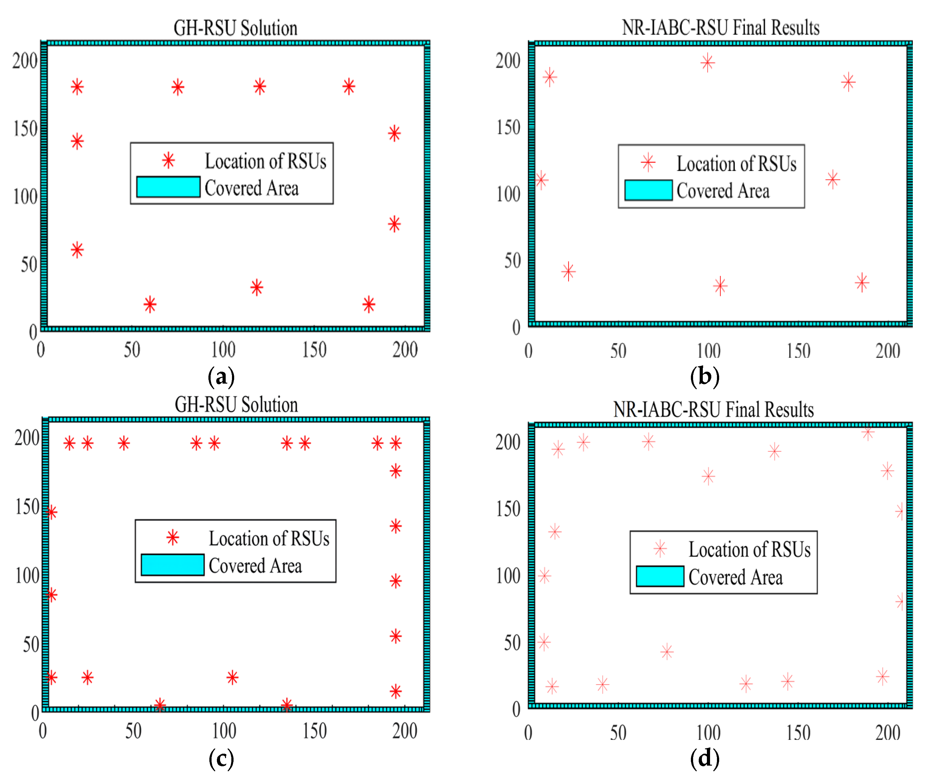
5.2.1. An Illustration of Deployment Results

Figure 4 shows an illustration of the deployment results of the two algorithms when $b_0$ is 1 and 2 under the same condition of Ds = 23 and λ = 0.1, respectively. The deployment result when $b_0=1$ is shown in Figure 4a,b, where it is observed that the number (8) of the RSUs deployed by NR-IABC is less than that (11) by GH. The deployment result when $b_0=2$ is shown in Figure 4c,d, it can be observed that the number (18) of RSUs deployed by NR-IABC is less than that (21) by GH, which indicates that the NR-IABC algorithm is cost-effective. Furthermore, according to Equations (14) and (24), $b_0$, λ, and Ds can all affect the deployment results. Therefore, to quantify the impact of the above parameters, we further present a set of experiments to compare the GH algorithm and NR-IABC algorithm.

Figure 4. An illustration of system deployment diagram: (a) $b_0=1$, GH; (b) $b_0=1$, NR-IABC; (c) $b_0=2$, GH; (d) $b_0=2$, NR-IABC.

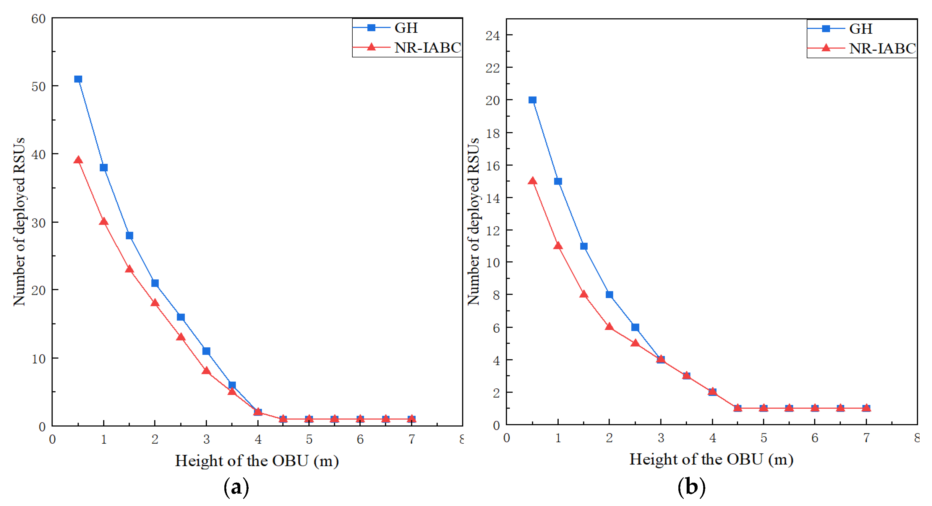
5.2.2. The Impact of Antenna Height

To illustrate the effect of $b_0$ on the RSUD problem, $b_0$ is set to be 0.5~7 m, respectively. The impact of $b_0$ under two different conditions (γ = 0.1, $D_s=23$; γ = 0.1, $D_s=33$) is shown in Figure 5. It can be observed that the number of RSUs deployed by GH and NR-IABC decreases with the growth of $b_0$ when $b_0\le 4$ and the decreasing trend of deployed RSUs gradually slows down with the growth of $b_0$. However, NR-IABC outperforms GH in all cases because fewer RSUs are deployed by NR-IABC, which can generally save 10% to 15%. The reason is that occlusion occurs when the height of the connection line between the top of the RSU and the OBU is less than 4 m, which requires the deployment of more RSUs to eliminate the impact of occlusion. When $b_0>4$, NR-IABC and GH gradually maintain a stable value with the increase in $b_0$. It indicates that the transmission of the signal is not affected, which corresponds to the LOS condition. Therefore, only one RSU can cover all of the target roads. The results show that to avoid the effect of truck occlusion, the antenna of the OBU should be raised or the RSU should be deployed at a high position to ensure that the connection between the OBU and the RSU is above the top of the truck as an obstacle.

Figure 5. The impact of different $b_0$ under two different conditions: (a) γ = 0.1, $D_s=23$; (b) γ = 0.1, $D_s=33$.

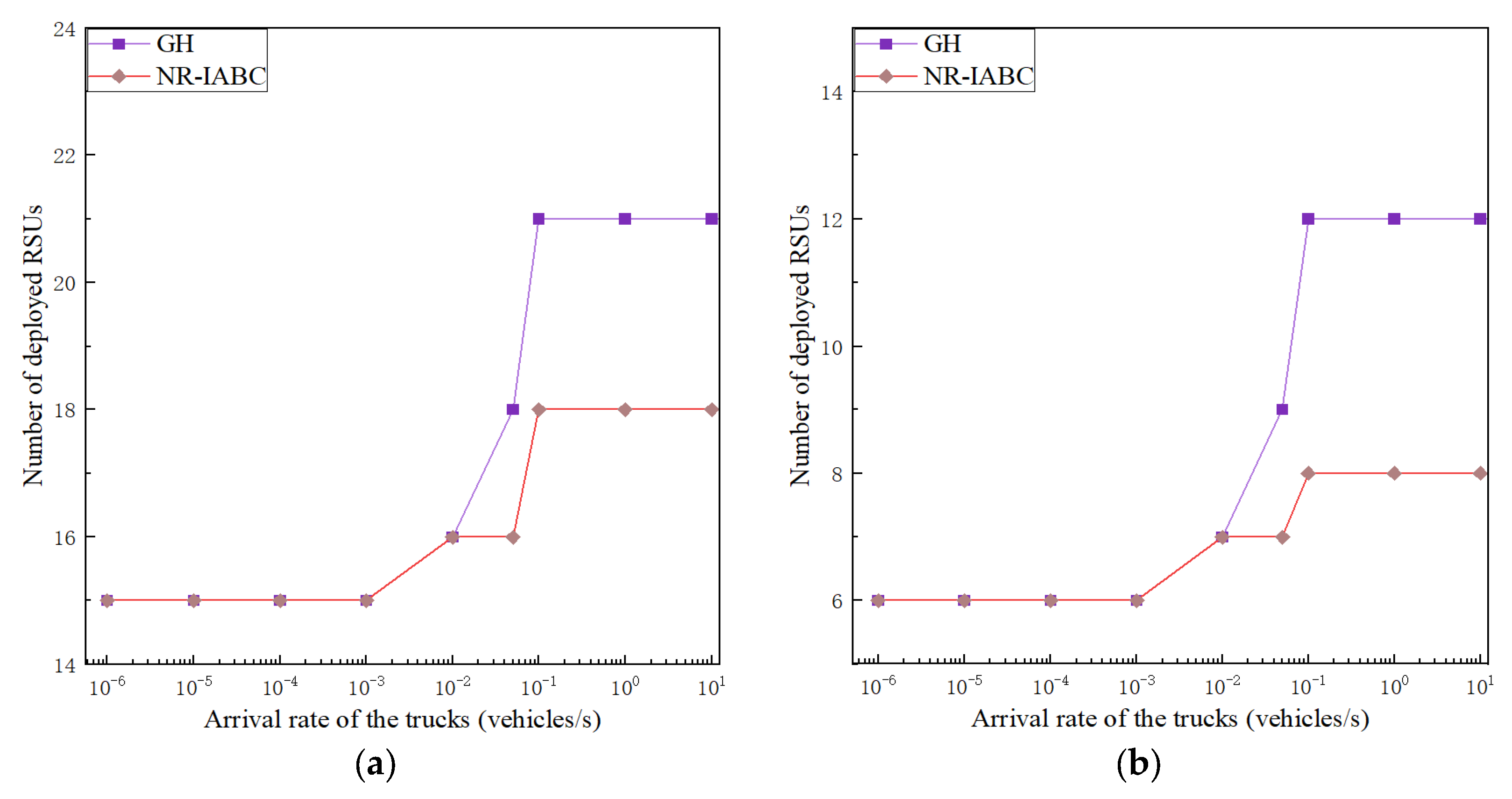
5.2.3. The Impact of Traffic Density

In order to study the effect of γ, we set γ to be ${10}^{-6}~10$ vehicles/s, respectively. The impact of γ under two different conditions ($b_0=2$, $D_s=23$; $b_0=3$, $D_s=23$) is shown in Figure 6. It is obvious that the number of deployed RSUs does not change when γ is less than 0.001, which indicates that occlusion hardly occurs. The gap between them gradually maintains a stable value when $\gamma >0.1$, which indicates that the probability of the occlusion has reached the upper limit. According to Equation (25), if $\exists \alpha ={\alpha }_0,{\alpha }_0\in [0,\frac{\pi }{2})$ makes $P_{nloss}^{NLOS}=1$, then $P_{nloss}=P_{NLOS}+P_{LOS}=1$ constantly holds when $\alpha \in \left[0,{\alpha }_0\right)$, which indicates the RSUs can cover $[0,{\alpha }_0)$ and the coverage range is not affected by γ, that is, the condition of $\gamma >0.1$. In addition, the number of RSUs deployed by NR-IABC has a faster growth rate than GH with the growth of γ when $0.001\le \gamma \le 0.1$ and this effect becomes stronger with the increase in γ. If $\forall \alpha \in [0,\frac{\pi }{2})$, $P_{nloss}^{NLOS}=0$ constantly satisfies, it can be deduced that $P_{nloss}=P_{LOS}\cdot P_{nloss}^{LOS}=P_{LOS}$ and $P_{LOS}$ is highly influenced by γ, which corresponds to the condition of $0.001\le \gamma \le 0.1$. Basically, $P_{nloss}$ is also limited by σ. Furthermore, $P_{nloss}$ can only be affected by γ if both of the following conditions are satisfied: one is the value of $d_0$ is proper so that $P_{LOS}\ge 0.9$ always holds and the other is that $P_{nloss}^{NLOS}=0$ constantly holds when $\alpha \in [0,\frac{\pi }{2})$. For further analysis, regardless of the value of $d_0$, $P_{LOS}<0.9$ constantly established when $\gamma >0.1$. Therefore, $P_{nloss}$ at this time may not be affected by γ. When $\gamma \le 0.1$, if $d_0>10$ is satisfied, $P_{nloss}$ may be affected by γ. In the NR-IABC algorithm, RSUs always tend to be deployed close to the roadside ($d_0$ is always less than 10), but in the GH algorithm, $d_0$ depends on the discrete granularity g, and a larger g can lead to a greater impact. In conclusion, γ has a significant impact on the result of the GH algorithm, while NR-IABC is slightly affected by γ.

Figure 6. The impact of different traffic density under two conditions: (a) $b_0=2$, $D_s=23$; (b) $b_0=3$, $D_s=23$.

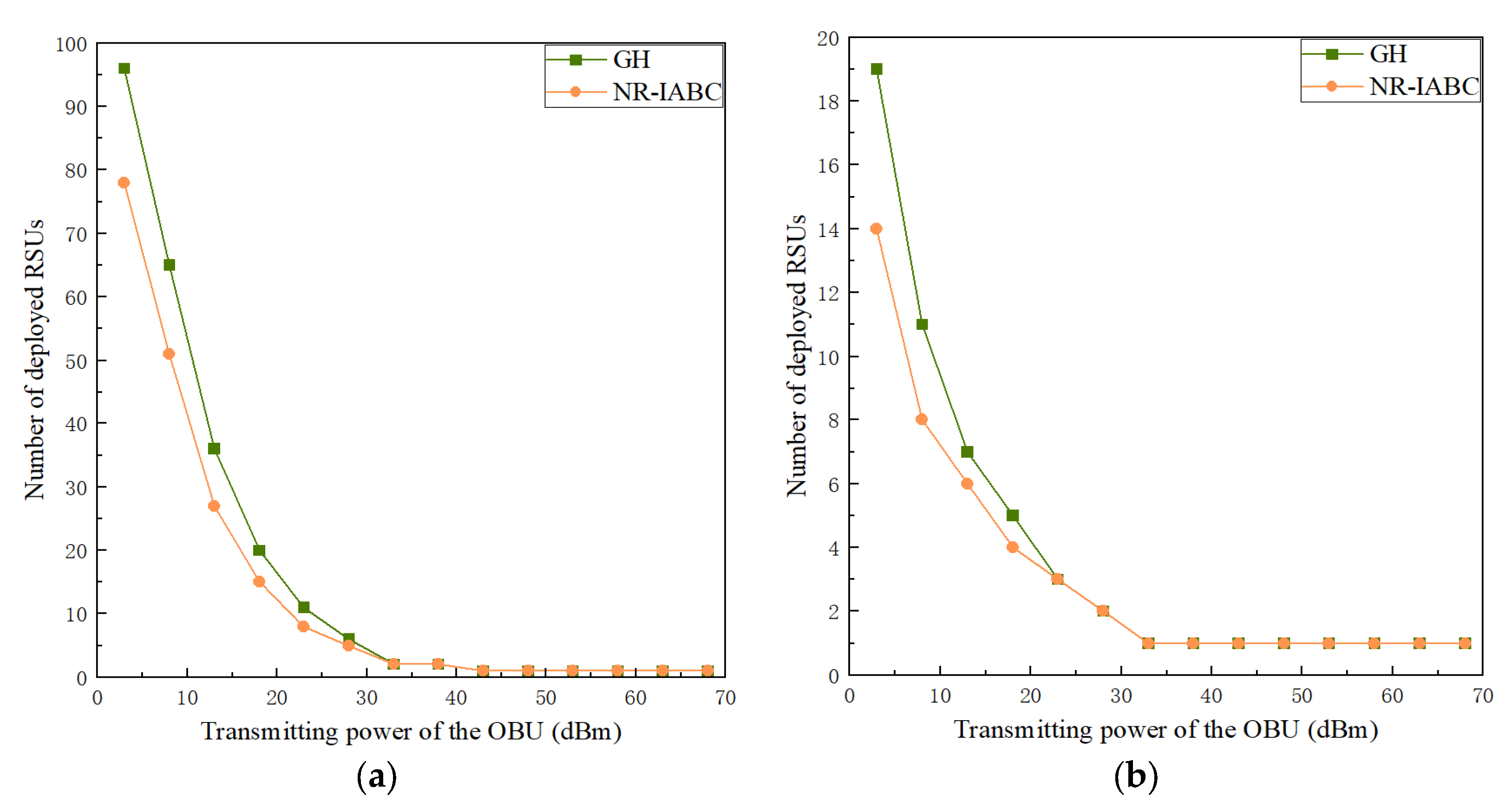
5.2.4. The Impact of Transmitting Power

The impact of $D_s$ under two different conditions ($b_0=3$, γ = 0.1; $b_0=3.5$, γ = 0.1) is shown in Figure 7. Results in Figure 7a,b both show that the number of deployed RSUs by GH or NR-IABC reduces with the growth of $D_s$, but NR-IABC outperforms GH in all cases, which can generally save 10% to 15%. The decreasing trend of deployed RSUs by the two algorithms gradually slows down with the growth of $D_s$, and they both maintain a fixed value when $D_s$ exceeds an upper limit. As an example, we only analyze the results in Figure 7a. Basically, when the value of $D_s$ is small enough as $D_s<-30dBm$, the RSUs have no coverage for the road. Then, we set $d_0=0$ under this condition, which corresponds to the smallest value of $LOS{S}_{NLOS}$, then $P_{nloss}=0$ is always established for all CPs. Obviously, the target road cannot be covered no matter how many RSUs are deployed. Moreover, when the value of $D_s$ is large enough as $D_s>40dBm$, only one RSU can cover all of the angle range within a road. Similarly, we set $d_0=200$ under this condition, which corresponds to the largest value of $LOS{S}_{NLOS}$, then $P_{nloss}=1$ is always established for all CPs. Therefore, only one RSU is needed to cover the whole road under the condition of $D_s>40dBm$.

Figure 7. The impact of different transmit power under two conditions: (a) $b_0=3$, γ = 0.1; (b) $b_0=3.5$, γ = 0.1.

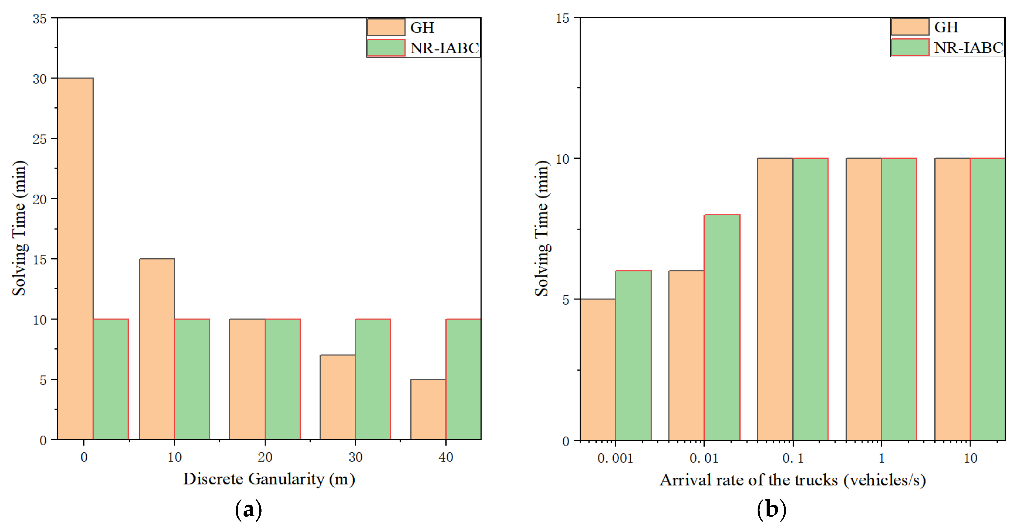
5.2.5. The Efficiency of Two Algorithms

We compared the solution efficiency of GH and NR-IABC under two different parameters in Figure 8. In Figure 8a, it can be observed that the solving time of GH increases significantly with the reduction in discrete granularity. In general, GH does have a faster solution speed than NR-IABC at a large discrete granularity, but a large discrete granularity will lead to the loss of precision. From Figure 8b, we can observe that the solving time by both two algorithms gradually increases with the growth of γ when γ is less than 0.1, and it tends to a stable value of 10 when γ is larger than 0.1. Combining the results of Figure 8, the solution efficiency of the two algorithms is comparable, but in the solution of large-scale problems, the NR-IABC algorithm has more advantages than the GH algorithm.

Figure 8. Time comparison between GH and NR-IABC under two different parameters: (a) discrete granularity (γ = 0.1); (b) arrival rate of the trucks (g = 20).

6. Conclusions

In this paper, a novel multi-objective optimization problem of roadside unit deployment under the constraints of target road coverage and communication reliability is proposed, and the influence of communication blocking caused by mobile vehicles on wireless communication is involved. By analyzing the NP-hardness of the problem, an Improved Artificial Bee Colony algorithm based on Neighborhood Ranking (NR-IABC) and a Greedy Heuristic (GH) algorithm are proposed to approximately solve the problem. Moreover, some methods, such as the “Neighborhood Ranking” method, combining the sensitivity and pheromone as the selection strategy, applying the mutual gravitation parameter to the interaction strategy, and replacing the worst nectar using the reverse learning method, are adopted to reduce the defects of strong randomness, where it is easy to fall into the local optimum and slow convergence speed of traditional Artificial Bee Colony algorithm. Then, real-life datasets are used to verify the scalability and efficiency of our proposed solutions. By comparative simulations on the key parameters, such as density of traffic flow, antenna height of OBU, and transmit power of OBU, the NR-IABC-based solution can always deploy fewer RSUs (usually 10~15%) and, thus, is more cost-effective compared with the GH based solution.

In the future, two aspects as an extension of this paper can be explored: First, we intend to test our approach on large-scale urban environments based on realistic traffic traces to further verify the performance of the proposed models and algorithms. Second, we will consider using intermediate obstacle vehicles or vehicles parked near buildings as relays, which can improve the utilization of resources and further reduce the deployment cost of RSUs.

References

1. Mahmood, D.A.; Horváth, G. Analysis of the Message Propagation Speed in VANET with Disconnected RSUs. Mathematics 2020, 8, 782. [Google Scholar] [CrossRef]
2. Zhou, H.B.; Xu, W.C.; Chen, J.C.; Wang, W. Evolutionary V2X Technologies Toward the Internet of Vehicles: Challenges and Opportunities. Proc. IEEE 2020, 108, 308–323. [Google Scholar] [CrossRef]
3. Quy, V.K.; Nam, V.H.; Linh, D.M.; Ban, N.T.; Han, N.D. Communication Solutions for Vehicle Ad-hoc Network in Smart Cities Environment: A Comprehensive Survey. Wirel. Pers. Commun. 2022, 122, 2791–2815. [Google Scholar] [CrossRef]
4. Alheeti, K.; Alaloosy, A.; Khalaf, H.; Alzahrani, A.; Al_Dosary, D. An Optimal Distribution of RSU for Improving Self-Driving Vehicle Connectivity. Comput. Mater. Contin. 2022, 70, 3311–3319. [Google Scholar] [CrossRef]
5. Maglogiannis, V.; Naudts, D.; Hadiwardoyo, S.; van den Akker, D.; Marquez-Barja, J.; Moerman, I. Experimental V2X Evaluation for C-V2X and ITS-G5 Technologies in a Real-Life Highway Environment. IEEE Trans. Netw. Serv. Manag. 2022, 19, 1521–1538. [Google Scholar] [CrossRef]
6. Ahmed, Z.; Naz, S.; Ahmed, J. Minimizing transmission delays in vehicular ad hoc networks by optimized placement of road-side unit. Wirel. Networks 2020, 26, 2905–2914. [Google Scholar] [CrossRef]
7. Gao, Z.G.; Wu, H.-C.; Cai, S.B.; Tan, G.Z. Tight Approximation Ratios of Two Greedy Algorithms for Optimal RSU Deployment in One-Dimensional VANETs. IEEE Trans. Veh. Technol. 2021, 70, 3–17. [Google Scholar] [CrossRef]
8. Yu, H.Y.; Liu, R.K.; Li, Z.H.; Ren, Y.L.; Jiang, H. An RSU Deployment Strategy Based on Traffic Demand in Vehicular Ad Hoc Networks (VANETs). IEEE Internet Things J. 2022, 9, 6496–6505. [Google Scholar] [CrossRef]
9. Shi, Y.J.; Lv, L.L.; Yu, H.; Yu, L.J.; Zhang, Z.H. A Center-Rule-Based Neighborhood Search Algorithm for Roadside Units Deployment in Emergency Scenarios. Mathematics 2020, 8, 1734. [Google Scholar] [CrossRef]
10. Ghorai, C.; Banerjee, I. A constrained Delaunay Triangulation based RSUs deployment strategy to cover a convex region with obstacles for maximizing communications probability between V2I. Veh. Commun. 2018, 13, 89–103. [Google Scholar] [CrossRef]
11. Boban, M.; Barros, J.; Tonguz, O.K. Geometry-Based Vehicle-to-Vehicle Channel Modeling for Large-Scale Simulation. IEEE Trans. Veh. Technol. 2014, 63, 4146–4164. [Google Scholar] [CrossRef]
12. Boban, M.; Vinhoza, T.T.V.; Ferreira, M.; Barros, J.; Tonguz, O.K. Impact of Vehicles as Obstacles in Vehicular Ad Hoc Networks. IEEE J. Sel. Areas Commun. 2011, 29, 15–28. [Google Scholar] [CrossRef]
13. Anbalagan, S.; Bashir, A.K.; Raja, G.; Dhanasekaran, P.; Vijayaraghavan, G.; Tariq, U.; Guizani, M. Machine-Learning-Based Efficient and Secure RSU Placement Mechanism for Software-Defined-IoV. IEEE Internet Things J. 2021, 8, 13950–13957. [Google Scholar] [CrossRef]
14. Liang, Y.Y.; Ma, N.; Li, X.; Hu, J. Stochastic Roadside Unit Location Optimization for Information Propagation in the Internet of Vehicles. IEEE Internet Things J. 2021, 8, 13316–13327. [Google Scholar] [CrossRef]
15. Selvakumari, P.; Sheela, D.; Chinnasamy, A. Chew’s Second Delaunay Triangulation Refinement Scheme for Optimal RSUs Deployment to Ensure Maximum Connectivity in Vehicle to Infrastructure Communication. Wirel. Pers. Commun. 2022, 123, 375–405. [Google Scholar] [CrossRef]
16. Guerna, A.; Bitam, S.; Calafate, C.T. AC-RDV: A novel ant colony system for roadside units deployment in vehicular ad hoc networks. Peer-to-Peer Netw. Appl. 2021, 14, 627–643. [Google Scholar] [CrossRef]
17. Lytaev, M.; Borisov, E.; Vladyko, A. V2I Propagation Loss Predictions in Simplified Urban Environment: A Two-Way Parabolic Equation Approach. Electronics 2020, 9, 2011. [Google Scholar] [CrossRef]
18. Li, W.; Hu, X.Y.; Gao, J.; Zhao, L.; Jiang, T. Measurements and Analysis of Propagation Channels in Vehicle-to-Infrastructure Scenarios. IEEE Trans. Veh. Technol. 2020, 69, 3550–3561. [Google Scholar] [CrossRef]
19. Kim, H.K.; Becerra, R.; Bolufé, S.; Azurdia-Meza, C.A.; Montejo-Sánchez, S.; Zabala-Blanco, D. Neuroevolution-Based Adaptive Antenna Array Beamforming Scheme to Improve the V2V Communication Performance at Intersections. Sensors 2021, 21, 2956. [Google Scholar] [CrossRef]
20. Eshteiwi, K.; Kaddoum, G.; Selim, B.; Gagnon, F. Impact of Co-Channel Interference and Vehicles as Obstacles on Full-Duplex V2V Cooperative Wireless Network. IEEE Trans. Veh. Technol. 2020, 69, 7503–7517. [Google Scholar] [CrossRef]
21. Hoque, M.A.; Rios-Torres, J.; Arvin, R.; Khattak, A.; Ahmed, S. The extent of reliability for vehicle-to-vehicle communication in safety critical applications: An experimental study. J. Intell. Transp. Syst. 2020, 24, 264–278. [Google Scholar] [CrossRef]
22. He, R.S.; Molisch, A.F.; Tufvesson, F.; Zhong, Z.D.; Ai, B.; Zhang, T.T. Vehicle-to-Vehicle Propagation Models with Large Vehicle Obstructions. IEEE Trans. Intell. Transp. Syst. 2014, 15, 2237–2248. [Google Scholar] [CrossRef]
23. Abbas, T.; Sjöberg, K.; Karedal, J.; Tufvesson, F. A Measurement Based Shadow Fading Model for Vehicle-to-Vehicle Network Simulations. Int. J. Antennas Propag. 2015, 2015, 1–12. [Google Scholar] [CrossRef]
24. Yang, L.; Wang, Y.B.; Yao, Z.H. A New Vehicle Arrival Prediction Model for Adaptive Signal Control in a Connected Vehicle Environment. IEEE Access 2020, 8, 112104–112112. [Google Scholar] [CrossRef]
25. Hmamouche, Y.; Benjillali, M.; Saoudi, S. Fresnel Line-of-Sight Probability with Applications in Airborne Platform-Assisted Communications. IEEE Trans. Veh. Technol. 2022, 71, 5060–5072. [Google Scholar] [CrossRef]
26. Braga, A.D.; Da Cruz, H.A.O.; Eras, L.E.C.; Araujo, J.P.L.; Neto, M.C.A.; Silva, D.K.N.; Cavalcante, G.P.S. Radio Propagation Models Based on Machine Learning Using Geometric Parameters for a Mixed City-River Path. IEEE Access 2020, 8, 146395–146407. [Google Scholar] [CrossRef]
27. Lopez-Benitez, M.; Zhang, J.Y. Comments and Corrections to “New Results on the Fluctuating Two-Ray Model with Arbitrary Fading Parameters and Its Applications”. IEEE Trans. Veh. Technol. 2021, 70, 1938–1940. [Google Scholar] [CrossRef]
28. Al-Absi, M.A.; Al-Absi, A.A.; Lee, H.J. Varied density of vehicles under city, highway and rural environments in V2V communication. Int. J. Sens. Networks 2020, 33, 148–158. [Google Scholar] [CrossRef]
29. Gao, Z.G.; Chen, D.J.; Cai, S.B.; Wu, H.-C. Optimal and Greedy Algorithms for the One-Dimensional RSU Deployment Problem with New Model. IEEE Trans. Veh. Technol. 2018, 67, 7643–7657. [Google Scholar] [CrossRef]
30. Yao, H.Q.; Zheng, C.Q.; Fu, X.W.; Yang, Y.S.; Ungurean, I. Charger and receiver deployment with delay constraint in mobile wireless rechargeable sensor networks. Ad Hoc Netw. 2022, 126, 102756. [Google Scholar] [CrossRef]
31. Wang, H.; Wang, W.J.; Xiao, S.Y.; Cui, Z.H.; Xu, M.Y.; Zhou, X.Y. Improving artificial Bee colony algorithm using a new neighborhood selection mechanism. Inf. Sci. 2020, 527, 227–240. [Google Scholar] [CrossRef]
32. Saeed, M.H.; Wang, F.Z.; Salem, S.; Khan, Y.A.; Kalwar, B.A.; Fars, A. Two-stage intelligent planning with improved artificial bee colony algorithm for a microgrid by considering the uncertainty of renewable sources. Energy Rep. 2021, 7, 8912–8928. [Google Scholar] [CrossRef]
33. Lin, P.; Wang, A.M.; Zhang, L.; Wu, J.; Sun, G.; Liu, L.L.; Lu, L. An improved cuckoo search with reverse learning and invasive weed operators for suppressing sidelobe level of antenna arrays. Int. J. Numer. Model. Electron. Netw. Devices Fields 2021, 34, e2829. [Google Scholar] [CrossRef]
34. Road Traffic Statistics. Available online: https://roadtraffic.dft.gov.uk/downloads (accessed on 20 August 2022).
35. Product Brochure of the Automotive Module (C-V2X AG15). Available online: https://www.quectel.com/product/c-v2x-ag15 (accessed on 20 August 2022).
Publisher’s Note: MDPI stays neutral with regard to jurisdictional claims in published maps and institutional affiliations.
Article Metrics
Citations
Article Access Statistics
Multiple requests from the same IP address are counted as one view.