Quality-Enhancing Techniques for Model-Based Reconstruction in Magnetic Particle Imaging

Abstract

Magnetic Particle Imaging is an imaging modality that exploits the non-linear magnetization response of superparamagnetic nanoparticles to a dynamic magnetic field. In the multivariate case, measurement-based reconstruction approaches are common and involve a system matrix whose acquisition is time consuming and needs to be repeated whenever the scanning setup changes. Our approach relies on reconstruction formulae derived from a mathematical model of the MPI signal encoding. A particular feature of the reconstruction formulae and the corresponding algorithms is that these are independent of the particular scanning trajectories. In this paper, we present basic ways of leveraging this independence property to enhance the quality of the reconstruction by merging data from different scans. In particular, we show how to combine scans of the same specimen under different rotation angles. We demonstrate the potential of the proposed techniques with numerical experiments.

1. Introduction

Magnetic Particle Imaging (MPI) is an emerging imaging modality which has become a vivid and interdisciplinary field of research since its introduction with the seminal work by Gleich and Weizenecker [1]. The imaging task of MPI is to reconstruct the spatial distribution of paramagnetic nanoparticles from measurements of a voltage induced by the non-linear magnetization response of these particles when a magnetic field is applied during an MPI scan. The magnetic particles are injected into the specimen before the scan. After reconstruction, the spatial distribution of the particles provides a means to visualize the interior of the specimen, e.g., the system of blood vessels. Potential applications of MPI entail tracer-based diagnostics such as cancer detection or blood flow imaging [2], or quantitative stem cell imaging [3]. Brain applications such as MPI-assisted stroke detection or monitoring may be feasible in the near future with a recently developed human-sized MPI scanner as demonstrated by [4].

MPI is an auspicious technique as it provides certain advantages compared with established imaging methods: (i) MPI offers high spatial and temporal resolution; (ii) in contrast to methods such as PET [5] or SPECT [6], the specimen is not exposed to radioactive tracers or radiation.

Regarding the reconstruction of the spatial distribution of the magnetic particles measurement-based approaches are common in the multivariate 2D and 3D setups. Such measurement-based approaches use a so-called system matrix which is acquired during a time-consuming procedure: every column of the system matrix corresponds to a voxel in the field of view and for every voxel a delta probe has to be scanned [7,8,9,10]. Scan data of a specimen provides the right-hand side of the linear system corresponding to the system matrix. Regularized inversion [11,12] of this linear system yields the reconstruction of the spatial particle distribution.

In common scan setups the physical field of view has usually a side length of about 10 mm. Enlarging the effective field of view is thus an important research topic. Currently, so-called multi-patch scan sequences [13,14] are employed which stitch together reconstructions of different patches.

Because the acquisition procedure outlined above is rather expensive, especially if high resolution reconstructions are requested in the multivariate case, model-based techniques are advisable. Model-based approaches to reconstruction have been considered in [15,16,17,18,19,20,21]. For the multivariate setup the early model-based algorithms essentially simulate the columns of the system matrix. Actual reconstruction formulae were given initially only for the 1D setup [15] by exploiting a relationship of the 1D model to Chebyshev polynomials. The authors’ preliminary work [22] has provided reconstruction formulae for the 2D and 3D scenarios. Moreover, Ref. [22] has demonstrated a first algorithm which is based on these reconstruction formulae and features two stages: Stage 1, the MPI core operator is estimated by employing a local least squares (LLSq) fit. Stage 2, the reconstruction of the spatial particle distribution is performed by regularized deconvolution of the result from Stage 1. In the conference paper [23], a variational approach to Stage 1 was proposed which makes the technique more flexible.

Regularization plays a prominent role regarding image reconstruction in general and MPI in particular. This is because either approach, measurement-based or model-based, provides an inverse problem which is ill-posed (or ill-conditioned in a discrete setting), i.e., we have to deal with severe amplification of measurement noise or other small perturbations contained in the measured data [24,25].

In this paper we propose a quality-enhancing technique based on the combination of multiple trajectories using a model-based reconstruction as introduced in [22]. More precisely, we make the following contributions: (i) extension of the algorithmic framework of [22,23], (ii) development of a model-based reconstruction scheme for quality-enhancement by combination of multiple scans along different trajectories, and (iii) demonstration of the technique’s potential by numerical experiments. Concerning (i), we extend the two-stage scheme of [22] by a TV-smooth regularization in Stage 2. This complements [23] whose focus was the variational inpainting-type reconstruction of Stage 1. Concerning (ii), the strategy for quality-enhancement relies on two facts: First, the model of [22] exhibits a beneficial feature, namely that is independent of the chosen scan trajectories. Second, the temporal causality of scan trajectories is not relevant to our algorithms since the data samples are processed as point cloud in extended phase space (measured data, position, velocity). These two features make it possible to combine the collected data from different scan trajectories for the model-based reconstruction scheme to enhance the quality of reconstructions. Different trajectories may be obtained via simple geometric transformations such as translations and rotations. In particular, we propose to employ rotations. We work out this case in detail. These rigid body transformations may also be emulated in practice without changing the settings of the MPI-scanner but by placing the specimen in a rotated or shifted position. We note that it may be advisable to practitioners to work with rotations, too. Moreover, we point out that data from multi-patch sequences which basically employ shifted versions of a standard scan trajectory can in principle be handled by our method. Finally, concerning (iii), we demonstrate the technique’s potential to enhance the quality of reconstructions through computational experiments with simulated data.

The paper is organized as follows: In Section 2 we collect the mathematical prerequisites; in particular, a concise review of the mathematical model of MPI and the reconstruction formulae is given. In Section 3 we present and extend the two-stage algorithmic model-based variational reconstruction framework proposed by the authors. More precisely, the mathematical structure and the variational formulation of the two-stage reconstruction are the topics of Section 3.1. In Section 3.2 we provide details on the numerical treatment of the mathematical subproblems. Section 4 explicates firstly the general merging property, i.e., how data from multiple scans can be combined within our model-based reconstruction technique. Secondly, it explains how scans of rotated versions of a specimen can be merged. In Section 5 we discuss the results of the computational experiments. We show with different experiments how the use of rotations can improve the reconstruction quality with respect to object shape as well as particle concentration. Finally, in Section 6 and Section 7 we provide a discussion and conclusions, respectively.

2. Materials and Methods

In this section we briefly review the mathematical model we employ; in particular, we discuss its analytical properties and the reconstruction formulae of [22] which we use in this paper.

2.1. Signal Encoding

Magnetic Particle Imaging exploits the non-linearity of the magnetization response from superparamagnetic particles to an applied magnetic field $H(x,t)\in {\mathbb{R}}^3$ which varies spatially and temporally. For a schematic on the measurement process we refer for instance to the authors’ paper [22] and to the book [2] for further details. The applied field $H(x,t)=Gx+H_D\left(t\right)$ is the superposition of a linear static field $Gx$ and a dynamic controllable drive field $H_D\left(t\right)$. In this article we consider the field free point (FFP) setup of an MPI scanner which is currently a commonly used setup (cf. [26]). In the FFP setup the matrix $G\in {\mathbb{R}}^{3\times 3}$ is non-singular. Consequently, the location where the applied field vanishes at time t is the unique point given by $r\left(t\right)=-G^{-1}{H}_D\left(t\right)\in {\mathbb{R}}^3$ and is called the field free point. Because the FFP is uniquely determined by the dynamic drive field $H_D\left(t\right)$ and also the other way around the drive field $H_D\left(t\right)=-Gr\left(t\right)$ by the FFP, the applied field can be expressed as $H(x,t)=G(x-r(t\left)\right)$ (cf. x-space formulation [18,19]), which we use here. After preparation with a solution of magnetic particles the specimen is placed in the field of view (FOV) of the MPI scanner. During the scan the field free point is a sensitive spot where the magnetization response of the particles has a steep rise in magnitude and thus a strong gradient. The magnetization response $M(x,t)\in {\mathbb{R}}^3$ is described by the Langevin theory of paramagnetism [27,28] and reads as

$$\begin{array}{cccc}\hfill M(x,t)& =\rho \left(x\right)m\mathcal{L}\left(\frac{\left|H\right(x,t\left)\right|}{H_{\mathrm{sat}}}\right)\frac{H(x,t)}{\left|H\right(x,t\left)\right|},\hfill & \hfill \mathcal{L}\left(\xi \right)& =coth\left(\xi \right)-\frac{1}{\xi }.\hfill \end{array}$$

(1)

Equation (1) involves different quantities which are: the spatial distribution $\rho$ of the magnetic particles, the magnetic moment m of a single particle, and $H_{\mathrm{sat}}$ which is a combined saturation parameter depending on the diameter and the saturation magnetization of the particles as well as on the temperature. The Langevin function $\mathcal{L}\left(\xi \right)$ is a sigmoid function with a steep rise at $\xi =0$. The magnetization response $M(x,t)$ is aligned with the applied field, but its magnitude is affected essentially by $\rho$ and $\mathcal{L}$.

An MPI scanner has typically three recording coils where the MPI data is measured. The measured data is the voltage induced in the recording coils stemming from the negative rate of change of the magnetic flux, according to Faraday’s law. With Faraday’s law the induced voltage is the superposition of two parts: the first part involves only the applied field, while the second part involves the magnetization response as of Equation (1). Because only the second part depends on $\rho$, i.e., the image which we want to reconstruct, we remove the first part by subtracting a reference signal from an empty scan. That is, after subtraction, we are given time-dependent data $s\left(t\right)\in {\mathbb{R}}^3$ which relates to the particle distribution $\rho$ by

$$\begin{array}{cc}\hfill s\left(t\right)& =-\frac{d}{dt}{\mu }_0\underset{{\mathbb{R}}^3}{\int }M(x,t)dx={\mu }_{0}m\frac{d}{dt}\underset{{\mathbb{R}}^3}{\int }\rho \left(x\right)\mathcal{L}\left(\frac{\left|G\right(r\left(t\right)-x\left)\right|}{H_{\mathrm{sat}}}\right)\frac{G\left(r\right(t)-x)}{\left|G\right(r\left(t\right)-x\left)\right|}dx.\hfill \end{array}$$

(2)

In other words, the underlying signal $\rho \left(x\right)$ is encoded in the data $s\left(t\right)$ via Equation (2).

2.2. MPI Core Operator and Reconstruction Formulae

We employ Equation (2) as basis for the reconstruction of the particle distribution $\rho \left(x\right)$ from measured data $s\left(t\right)$. To this end, we transform and non-dimensional Equation (2) into the following more convenient form

$$\begin{array}{cc}\hfill s\left(t\right)& =\frac{d}{dt}\underset{{\mathbb{R}}^3}{\int }\rho \left(x\right)\mathcal{L}\left(\frac{\left|r\right(t)-x|}{h}\right)\frac{r\left(t\right)-x}{\left|r\right(t)-x|}dx.\hfill \end{array}$$

(3)

This transformation is achieved by a change of variables (cf. [22] for the details). The remaining quantities are then dimensionless and we reuse the previous symbols to denote them as well. The parameter $h>0$ is also dimensionless and constitutes a resolution parameter. From Equation (3) we infer the MPI Core Operator $A\left[\rho \right]\left(r\right)\in {\mathbb{R}}^{3\times 3}$ which reads as

$$\begin{array}{cccc}\hfill s\left(t\right)& =A\left[\rho \right]\left(r\left(t\right)\right)r^{\prime }\left(t\right),\hfill & \hfill A\left[\rho \right]\left(r\right)& =\underset{{\mathbb{R}}^3}{\int }\rho \left(x\right){\nabla }_r\left(\mathcal{L}\left(\frac{|r-x|}{h}\right)\frac{r-x}{|r-x|}\right)dx.\hfill \end{array}$$

(4)

Here we want to emphasize that the MPI Core Operator $A\left[\rho \right]\left(r\right)$ does not depend on the particular choice of the scanning trajectory $t\to r\left(t\right),$ but only on the point $r=r\left(t\right).$ A further insight of [22] has been that the trace of the matrix valued core operator $A\left[\rho \right]\left(r\right)$ contains all information about $\rho \left(x\right)$. Moreover, the trace of $A\left[\rho \right]\left(r\right)$ is related to $\rho$ via convolution ${\kappa }_h\ast \rho$ with the kernel ${\kappa }_h$ as follows

$$\begin{array}{cccc}\hfill {\kappa }_h\ast \rho & =trace\left(A\left[\rho \right]\right),\hfill & \hfill \mathrm{where}{\kappa }_h\left(y\right)& =div\left(\mathcal{L}\left(\frac{\left|y\right|}{h}\right)\frac{y}{\left|y\right|}\right).\hfill \end{array}$$

(5)

Equation (5) implies the following reconstruction formula: let data $u=trace\left(A\left[\rho \right]\right)$ be given, then we obtain $\rho$ from deconvolution of u with the kernel ${\kappa }_h$. We point out that the regularized variant of this reconstruction formula is a key ingredient for the algorithmic reconstruction scheme below; cf. Equation (9). Moreover, the kernel is an analytic function on ${\mathbb{R}}^3$, cf. [22].

3. Algorithmic Framework and Numerical Realization

In this section we recall and extend an algorithmic model-based reconstruction framework proposed by the authors in [23] which is based on the above reconstruction formulae in Equation (5) using suitable regularization. In particular, we describe a two stage scheme for which we provide both the variational models as well as information on discretization and concrete numerical realization.

3.1. Model-Based Reconstruction Framework

Equations (4) and (5) state the mathematical relationships between the measured data, the MPI Core Operator $A\left[\rho \right]\left(r\right)$ and the distribution $\rho \left(x\right)$ of particles. They form the basis of a model-based algorithmic framework consisting of two stages. Stage 1 implements the reconstruction of the MPI Core Operator $A\left[\rho \right]\left(r\right)$ using Equation (4). Stage 2 implements the reconstruction of $\rho \left(x\right)$ using Equation (5) with data $u=traceA\left[\rho \right]$ obtained in Stage 1. We point out that in algorithmic realizations regularization is necessary due to ill-posedness (cf. [22]). In what follows we discuss the details of these two stages.

Stage 1: Reconstruction of the MPI Core Operator. The aim is to reconstruct the MPI Core Operator $A\left[\rho \right]\left(r\right)$ from a time series of measured data $s_k=s\left(t_k\right)$. By Equation (4), the data is related to a sampling of the core operator as follows

$$\begin{array}{cc}\hfill s_k& =A\left[\rho \right]\left(r_k\right)v_k,\mathrm{for}k\in \{1,\dots ,L\},\hfill \end{array}$$

(6)

where $r_k=r\left(t_k\right)$ and $v_k=r^{\prime }\left(t_k\right)$ denote the corresponding samples of the scan trajectory and the velocity, respectively.

We have two different approaches for the reconstruction of $A\left[\rho \right]\left(r\right)$ on a grid over the FOV: the Local Least Squares (LLSq) of [22] and the variational approach of [23]. With the LLSq technique all cells (pixels or voxels) are treated independently and samples $s_k,v_k$ are associated with a cell $C_i$ (or its center $x_i$) whenever the corresponding position $r_k$ is located in $C_i$. For every cell $C_i$ we collect the associated data samples $s_k$ as columns of the matrix $S_i$ and accordingly the velocities $v_k$ as columns of the matrix $V_i$. With the additional assumption that the matrix field A is constant on each cell $C_i$, we obtain $A_i\approx A\left[\rho \right]\left(x_i\right)$ as the least squares solution of

$$\begin{array}{cc}\hfill S_i& =A_i{V}_i.\hfill \end{array}$$

(7)

The trace field, i.e., the piecewise constant scalar field $u_i=trace\left(A_i\right)$ is the data for the second stage. Note that the LLSq approach will only work on grids defined such that each grid cell $C_i$ contains at least two data points. The latter condition can be restrictive in the case of unevenly or sparsely sampled data.

In [23] we proposed a variational (inpainting type) approach to reconstruct the core operator which does not impose restrictions on the grid; in particular, it is not required that each grid cell contains sufficient data. We obtain the estimate for the core operator A as the minimizer of the following functional $J\left[A\right],$ i.e.,

$$\begin{array}{cccc}\hfill A& =arg\underset{\widehat{A}}{min}J\left[\widehat{A}\right],\hfill & \hfill \mathrm{where}J\left[\widehat{A}\right]& =\underset{=:R\left[\widehat{A}\right]}{\underbrace{\frac{\lambda }{N}{\parallel D\widehat{A}\parallel }_2^2}}+\underset{=:F\left[\widehat{A}\right]}{\underbrace{\frac{1}{L}\sum _{k=1}^L{\left|s_k-I\left[\widehat{A}\right]\left(r_k\right)v_k\right|}^2}}.\hfill \end{array}$$

(8)

Here, N denotes the number of total cells, and L the number of data samples. The argument $\widehat{A}$ is again constant on each grid cell. The matrix D is given as the discretization of the gradient operator by first differences. Thus, the regularizing term $R\left[\widehat{A}\right]$ given by the left-hand summand in Equation (8) enforces smoothness and fills small gaps by taking a neighborhood relationship between cells into account. The symbol $\lambda >0$ is a regularization parameter (hyperparameter) regulating the trade-off between regularization and data-fidelity. The data fidelity term $F\left[\widehat{A}\right]$ given by the right-hand summand in Equation (8) enforces the closeness of the approximation $\widehat{A}$ to the data. Here, the symbol $I\left[A\right]$ denotes the application of an interpolation scheme to the approximation A (such that $I\left[A\right]$ is a sufficiently smooth function defined on a continuous spatial domain). Hence, using $I\left[\widehat{A}\right],$ the summands of the fidelity term can be evaluated at the exact sample location $r_k$. In this paper, we employ bicubic interpolation to implement I.

Stage 2: Reconstruction of the Spatial Particle Distribution. We obtain the spatial particle distribution $\rho$ via regularized deconvolution, i.e., $\rho$ is the minimizer of the energy minimization problem

$$\begin{array}{cccc}\hfill \rho & =\underset{\widehat{\rho }}{argmin}E\left[\widehat{\rho }\right],\hfill & \hfill \mathrm{where}E\left[\widehat{\rho }\right]& ={||{\kappa }_h\ast \widehat{\rho }-u||}_2^2+\mu R\left[\widehat{\rho }\right].\hfill \end{array}$$

(9)

Here the residual of Equation (5), i.e., the squared euclidean norm of ${\kappa }_h\ast \widehat{\rho }-u$, provides the data fidelity with $u=trace\left(I\left[A\right]\right)$ being the trace field obtained in stage one. The hyperparameter $\mu >0$ denotes the regularization weight. The symbol $R\left[\widehat{\rho }\right]$ is used to denote a regularizer. Concrete realizations of R are discussed next.

In [23] we used the regularizer

$$\begin{array}{c}\hfill R\left[\rho \right]={||\nabla \rho ||}_2^2\end{array}$$

(10)

which leads to a standard Tikhonov regularizer for $\rho \in W^{1,2}\left(\mathsf{\Omega }\right)$, where $W^{k,p}\left(\mathsf{\Omega }\right)$ denotes the Sobolev space of differentiation order k and integration order p, and which enforces smoothness of the reconstruction.

In this paper we also employ Total Variation (TV) type regularization. More precisely, we use the TV-smooth regularizer (which is a standard regularizer used in imaging; cf. [24,29,30]). For a concentration $\rho$ of bounded variation, i.e., $\rho \in \mathrm{BV}\left(\mathsf{\Omega }\right)$ on a domain $\mathsf{\Omega },$ and $\delta >0$ it is given by

$$\begin{array}{cc}\hfill R_{\delta }\left[\rho \right]=sup\{\underset{\mathsf{\Omega }}{\int }& {\delta }^{\frac{1}{2}}{\phi }_0\left(x\right)-div\left(\phi \left(x\right)\right)\rho \left(x\right)dx:\hfill \\ \hfill & {\phi }_0\in C_c^1\left(\mathsf{\Omega }\right),\phi \in C_c^1\left(\mathsf{\Omega },{\mathbb{R}}^2\right),{\phi }_0^2+{\left|\phi \right|}^2\le 1\}.\hfill \end{array}$$

(11)

For $\rho \in W^{1,1}\left(\mathsf{\Omega }\right)\subset \mathrm{BV}\left(\mathsf{\Omega }\right)$ this expression reduces to

$$\begin{array}{cc}\hfill R_{\delta }\left[\rho \right]& =\underset{\mathsf{\Omega }}{\int }\sqrt{\delta +{|\nabla \rho \left(x\right)|}^2}dx.\hfill \end{array}$$

(12)

We observe that with $\delta \to 0$ the regularizer $R_{\delta }\left[\rho \right]$ approaches the total variation of $\rho$ denoted by ${\left|\rho \right|}_{\mathrm{TV}}$.

3.2. Discretization and Numerical Realization

We describe the numerical treatment of the considered energy minimization problems given by Equations (8) and (9) with Tikhonov regularization (10) and TV type regularization (11) in the two-dimensional case here. (The treatment of the three-dimensional case is similar but, from the view-point of notation, more involved).

In the 2D case the FOV is the box $\mathsf{\Omega }={[-1,1]}^2$ on which we define an $N_x\times N_y$ Cartesian grid. The $(i,j)$-th grid cell (or pixel) is represented by its center point $(x_i,y_j)\in \mathsf{\Omega }$, which explicitly read

$$\begin{array}{cccc}\hfill x_i& =-1+\left(i+\frac{1}{2}\right)h_x,\hfill & \hfill y_j& =-1+\left(j+\frac{1}{2}\right)h_y,\hfill \end{array}$$

(13)

where $h_x=\frac{2}{N_x}$ and $h_y=\frac{2}{N_y}$, for $i\in \{0,\dots ,N_x-1\}$ and $j\in \{0,\dots ,N_y-1\}$.

Numerical Approach for Stage 1: Reconstruction of the MPI Core Operator. The grid functions which approximate the MPI Core Operator are tensors $\widehat{A}\in {\mathbb{R}}^{N_x\times N_y\times 2\times 2}$, $\widehat{A}=\left({\widehat{A}}_{i,j}^{p,q}\right)$, where $i,j$ are the cell indices and $p,q$ the indices of the matrix components. The regularizing term $R\left[\widehat{A}\right]$ in Equation (8) was given by $R\left[\widehat{A}\right]=\frac{\lambda }{N}{\parallel D\widehat{A}\parallel }_2^2$ where we can more explicitly represent $\parallel D\widehat{A}{\parallel }_2^2$ by

$$\begin{array}{cc}\hfill {\parallel D\widehat{A}\parallel }_2^2& =\sum _{i=0}^{N_x-1}\sum _{j=0}^{N_y-1}\left({∥\frac{{\widehat{A}}_{i+1,j}-{\widehat{A}}_{i,j}}{h_x}∥}_F^2+{∥\frac{{\widehat{A}}_{i,j+1}-{\widehat{A}}_{i,j}}{h_y}∥}_F^2\right).\hfill \end{array}$$

(14)

Using this representation, we find the minimizer $A\in {\mathbb{R}}^{N_x\times N_y\times 2\times 2}$ of the functional J corresponding to Equation (8) by solving the gradient system $\nabla J\left[A\right]=0.$ This system is linear with respect to A. According to [23], the partial derivatives of the data fidelity term F of $J=R+F$ (cf. Equation (8)) are given by

$$\begin{array}{cc}\hfill \frac{\partial F\left[A\right]}{\partial A_{i,j}^{p,q}}& =-\frac{2}{L}\sum _{k=1}^L⟨s_k-I\left[A\right]\left(r_k\right)v_k,I\left[{\delta }_{i,j}^{p,q}\right]\left(r_k\right)v_k⟩,\hfill \end{array}$$

(15)

where ${\delta }_{i,j}^{p,q}$ denotes the Kronecker symbol, while those of the regularizing term read as

$$\begin{array}{cc}\hfill \frac{\partial R\left[A\right]}{\partial A_{i,j}^{p,q}}& =-\frac{2\lambda }{N}\left(\frac{A_{i-1,j}^{p,q}-2A_{i,j}^{p,q}+A_{i+1,j}^{p,q}}{h_x^2}+\frac{A_{i,j}^{p,q}-2A_{i,j}^{p,q}+A_{i,j+1}^{p,q}}{h_y^2}\right).\hfill \end{array}$$

(16)

The data fidelity term F of Equation (8) depends on the interpolation operation $I\left[A\right]\left(r\right)$. We use bicubic interpolation, meaning that, if the point to be evaluated $(r_x,r_y)$ is contained in the cell with center $(x_i,y_j)$, the evaluation is given as follows:

$$\begin{array}{cc}\hfill I\left[A^{p,q}\right](r_x,r_y)=& {\left(\begin{array}{c}{L}_{-1}\left(s_x\right)\\ L_0\left(s_x\right)\\ L_{+1}\left(s_x\right)\\ L_{+2}\left(s_x\right)\end{array}\right)}^T\left(\begin{array}{cccc}{A}_{i-1,j-1}^{p,q}& A_{i-1,j}^{p,q}& A_{i-1,j+1}^{p,q}& A_{i-1,j+2}^{p,q}\\ A_{i,j-1}^{p,q}& A_{i,j}^{p,q}& A_{i,j+1}^{p,q}& A_{i,j+2}^{p,q}\\ A_{i+1,j-1}^{p,q}& A_{i+1,j}^{p,q}& A_{i+1,j+1}^{p,q}& A_{i+1,j+2}^{p,q}\\ A_{i+2,j-1}^{p,q}& A_{i+2,j}^{p,q}& A_{i+2,j+1}^{p,q}& A_{i+2,j+2}^{p,q}\end{array}\right)\left(\begin{array}{c}{L}_{-1}\left(s_y\right)\\ L_0\left(s_y\right)\\ L_{+1}\left(s_y\right)\\ L_{+2}\left(s_y\right)\end{array}\right).\hfill \end{array}$$

(17)

Here the right-hand side is given via the Lagrange polynomials

$$\begin{array}{cccc}\hfill L_{-1}\left(s\right)& =-\frac{1}{6}s(s-1)(s-2),\hfill & \hfill L_0\left(s\right)& =\frac{1}{2}(s+1)(s-1)(s-2),\hfill \end{array}$$

(18)

$$\begin{array}{cccc}\hfill L_{+1}\left(s\right)& =-\frac{1}{2}s(s+1)(s-2),\hfill & \hfill L_{+2}\left(s\right)& =\frac{1}{6}s(s+1)(s-1),\hfill \end{array}$$

(19)

where $s_x=\frac{r_x-x_i}{h_x}$ and $s_y=\frac{r_y-y_j}{h_y}$ are the coordinates of $(r_x,r_y)$ relative to the cell. Note that the interpolation scheme acts independently on the matrix entries, i.e., $I\left[A\right](r_x,r_y)$ is obtained applying Equation (17) to every matrix component. The gradient system $\nabla J\left[A\right]=0$, can formally be written as a non-homogeneous linear system $GA=b$ (cf. [23]) with

$$\begin{array}{cc}\hfill {\left(GA\right)}_{i,j}^{p,q}& =\frac{2}{L}\sum _{k=1}^L⟨I\left[A\right]\left(r_k\right)v_k,I\left[{\delta }_{i,j}^{p,q}\right]\left(r_k\right)v_k⟩+\frac{\partial R\left[A\right]}{\partial A_{i,j}^{p,q}},\hfill \end{array}$$

(20)

$$\begin{array}{cc}\hfill b_{i,j}^{p,q}& =\frac{2}{L}\sum _{k=1}^L⟨s_k,I\left[{\delta }_{i,j}^{p,q}\right]\left(r_k\right)v_k⟩.\hfill \end{array}$$

(21)

Because the formal matrix G is the Hessian of a convex quadratic function it is symmetric positive definite. Thus, we may solve the linear system $GA=b$ with respect to A by using the conjugate gradient method [31].

Numerical Approach for Stage 2: Reconstruction of the Spatial Particle Distribution. Regarding the second stage, i.e., the reconstruction of spatial particle distribution by regularized deconvolution via the variational model Equation (9), the grid functions are of type $\rho \in {\mathbb{R}}^{N_x\times N_y}$ with ${\rho }_{i,j}\approx \rho (x_i,y_j)$. By the assumption that the support of $\rho$ is contained in the FOV $\mathsf{\Omega }$, the convolution integral ${\kappa }_h\ast \rho$ in the energy $E\left[\rho \right]$ of Equation (9) reduces to an integral over $\mathsf{\Omega }$, i.e.,

$$\begin{array}{cc}\hfill {\kappa }_h\ast \rho \left(x\right)& =\underset{\mathsf{\Omega }}{\int }\rho \left(y\right){\kappa }_h(x-y)dy.\hfill \end{array}$$

(22)

We approximate the integral in Equation (22) with the midpoint rule. The kernel ${\kappa }_h$ is sampled on the same grid as $\rho$ (but with appropriate extension) and the remaining summation is handled by FFT-based discrete convolution, giving us a discrete linear operator $K_h\rho \approx {\kappa }_h\ast \rho$. Note also that since ${\kappa }_h(-x)={\kappa }_h\left(x\right)$ (cf. [22]) the matrix $K_h$ is symmetric.

When we apply standard Tikhonov regularization, i.e., we use the regularizer $R\left[\rho \right]={||\nabla \rho ||}_2^2$ of Equation (10) in the deconvolution model in Equation (9), we discretize the regularizer by

$$\begin{array}{cc}\hfill R\left[\rho \right]& =h_x{h}_y\sum _{i=0}^{N_x-1}\sum _{j=0}^{N_y-1}{W}_{ij}.\hfill \end{array}$$

(23)

Here the summands $W_{ij}$ are given by

$$\begin{array}{cc}\hfill W_{ij}:=& \frac{{\left(D_x^{+}{\rho }_{i,j}\right)}^2+{\left(D_x^{-}{\rho }_{i,j}\right)}^2}{2}+\frac{{\left(D_y^{+}{\rho }_{i,j}\right)}^2+{\left(D_y^{-}{\rho }_{i,j}\right)}^2}{2},\hfill \end{array}$$

(24)

with the forward and backward first order difference operators defined by

$$\begin{array}{cccc}\hfill D_x^{+}{\rho }_{i,j}:=& \frac{{\rho }_{i+1,j}-{\rho }_{i,j}}{h_x},\hfill & \hfill D_x^{-}{\rho }_{i,j}:=& \frac{{\rho }_{i,j}-{\rho }_{i-1,j}}{h_x}.\hfill \end{array}$$

(25)

The averages in Equation (24) gives us formally second order accurate approximations at the cell centers, i.e.,

$$\begin{array}{cc}\hfill \frac{{\left(D_x^{+}{\rho }_{i,j}\right)}^2+{\left(D_x^{-}{\rho }_{i,j}\right)}^2}{2}& ={\partial }_x\rho {(x_i,y_j)}^2+O\left(h_x^2\right).\hfill \end{array}$$

(26)

Moreover, boundary conditions are implemented via padding of $\rho$. Concretely, we use zero-padding of $\rho$ which implements Dirichlet-zero boundary conditions and which is consistent with the assumption that the support of $\rho$ is contained in $\mathsf{\Omega }$. (We point out that other boundary conditions may be implemented as well.) We find the vectorized $\rho \in {\mathbb{R}}^{N_x·N_y}$ by solving the gradient system $\nabla E\left[\rho \right]=0$ of the discretized energy E which reads

$$\begin{array}{cc}\hfill -\mu L\rho +K_h^T(K_h\rho -u)& =0.\hfill \end{array}$$

(27)

Here L is the matrix of the discrete five-point stencil Laplacian (cf. [22]). The linear system features a symmetric positive definite matrix such that we may solve it with the conjugate gradient method.

In the case of TV-smooth regularization, i.e., we use the regularizer of Equation (11) in the deconvolution model in Equation (9), the discrete regularizer is given by

$$\begin{array}{cc}\hfill R_{\delta }\left[\rho \right]& =h_x{h}_y\sum _{i=0}^{N_x-1}\sum _{j=0}^{N_y-1}\sqrt{\delta +W_{ij}},\hfill \end{array}$$

(28)

with $W_{ij}$ as defined in Equation (24) (and zero-padding of $\rho$). The partial derivatives of $R_{\delta }\left[\rho \right]$ are expressed as

$$\begin{array}{cc}\hfill \frac{\partial R_{\delta }}{\partial {\rho }_{i,j}}\left[\rho \right]=& -\frac{A_x^{+}{g}_{i,j}{D}_x^{+}{\rho }_{i,j}-A_x^{-}{g}_{i,j}{D}_x^{-}{\rho }_{i,j}}{h_x}-\frac{A_y^{+}{g}_{i,j}{D}_y^{+}{\rho }_{i,j}-A_y^{-}{g}_{i,j}{D}_y^{-}{\rho }_{i,j}}{h_y}\hfill \\ \hfill g_{i,j}& =\frac{1}{\sqrt{\delta +W}}\hfill \end{array}$$

(29)

where the forward and backward average operators applied to the grid function g are

$$\begin{array}{cccc}\hfill A_x^{+}{g}_{i,j}:=& \frac{g_{i+1,j}+g_{i,j}}{2},\hfill & \hfill A_x^{-}{g}_{i,j}:=& \frac{g_{i,j}+g_{i-1,j}}{2}.\hfill \end{array}$$

(30)

We like to mention that Equation (29) is consistent with $-div\left(\nabla \rho /\sqrt{\delta +{|\nabla \rho |}^2}\right)$ which is the partial differential obtained by the calculus of variations. If D denotes again the first difference matrix corresponding to the gradient operator and $M\left[\rho \right]$ the diagonal matrix corresponding to the multiplication with $g=1/\sqrt{\delta +{|\nabla \rho |}^2}$, then we have

$$\begin{array}{cc}\hfill \nabla R_{\delta }\left[\rho \right]& =-D^{T}M\left[\rho \right]D\rho .\hfill \end{array}$$

(31)

With Equation (31) the gradient system $\nabla E\left[\rho \right]=0$ in the case of TV-smooth regularization reads as

$$\begin{array}{cc}\hfill -\mu D^{T}M\left[\rho \right]D\rho +K_h^T(K_h\rho -u)& =0.\hfill \end{array}$$

(32)

We solve Equation (32) by fixed point iteration as suggested by [29,30], i.e.,

$$\begin{array}{cccc}\hfill -\mu D^{T}M\left[{\rho }_k\right]D{\rho }_{k+1}+K_h^T(K_h{\rho }_{k+1}-u)& =0,\hfill & \hfill \mathrm{starting}\mathrm{with}{\rho }_0& =u.\hfill \end{array}$$

(33)

In every iteration we have a linear system with symmetric positive definite matrix which we solve using the conjugate gradient method.

4. Model-Based Reconstruction for Combining Multiple Scans

In this section, we describe how to incorporate an acquisition process based on geometric transformations which we propose for the quality-enhancement of reconstructions. In connection with this, we describe how corresponding simulated data can be generated.

General Merging Property. Our model-based approach comes with the feature that is does not depend on a particular choice of trajectory. The algorithm handles the data $(s_k,r_k,v_k)=$ (measured data, location, velocity) as point cloud in extended phase space. The data fidelity term in Equation (8) takes into account any provided data no matter which scan of the same object the data came from. Morever, the order of summation in the fidelity term may be arbitrary, which means that any temporal causalities that the data once had are not relevant. This gives us the freedom to merge data from scans of the same object acquired with different scan trajectories before the algorithm is applied. More precisely, let scan data sets $T_i$, $i\in \{1,\dots ,n\}$ of the same object along n different scan trajectories be given as

$$\begin{array}{cc}\hfill T_i& =\left\{\left(s_k^i,r_k^i,v_k^i\right):k\in \{1,\dots ,L_i\}\right\}\hfill \end{array}$$

(34)

then the merged data set T is the union

$$\begin{array}{cc}\hfill T& =\bigcup _{i=1}^n{T}_i\hfill \end{array}$$

(35)

and the algorithm is supplied with T.

Merging Scans from Rotated Versions of a Specimen. We propose here not to change the scan trajectory but instead to scan the specimen in rotated positions. With a change of variables this is equivalent to scanning along the reversely rotated version of the original scan trajectory. Consider a rotation matrix $Q_{\alpha }$ corresponding to a rotation angle $\alpha$. Placing the specimen rotated by $\alpha$ into the scanner means that we scan the rotated particle distribution $\widehat{\rho }\left(x\right)=\rho \left(Q_{\alpha }^{T}x\right)$. Following Equation (4) we obtain the data

$$\begin{array}{cc}\hfill \widehat{s}\left(t\right)& =A\left[\widehat{\rho }\right]\left(r\left(t\right)\right)v\left(t\right),\hfill \end{array}$$

(36)

with the core operator $A\left[\widehat{\rho }\right]$ applied to the rotated distribution $\widehat{\rho }$. By performing the change of variables $y=Q_{\alpha }^{T}x$ on the integral of Equation (4) which defines the core operator we obtain

$$\begin{array}{cc}\hfill \widehat{s}\left(t\right)& =Q_{\alpha }A\left[\rho \right]\left(Q_{\alpha }^{T}r\left(t\right)\right)Q_{\alpha }^{T}v\left(t\right),\hfill \end{array}$$

(37)

with the core operator $A\left[\rho \right]$ applied to the original distribution $\rho$. That means that the reversely rotated data $Q_{\alpha }^T\widehat{s}\left(t\right)$ corresponds to the original distribution $\rho$ but scanned along the reversely rotated trajectory $Q_{\alpha }^{T}r\left(t\right)$ with reversely rotated velocity $Q_{\alpha }^{T}v\left(t\right)$.

We exploit this property as follows: given a choice of rotation angles ${\alpha }_i$, we acquire for every angle scan data $(s_k,r_k,v_k)$ of the ${\alpha }_i$-rotated object. Then, we merge from each such scan the reversely rotated data $(Q_{{\alpha }_i}^T{s}_k,Q_{{\alpha }_i}^T{r}_k,Q_{{\alpha }_i}^T{v}_k)$, feed it into our two-stage reconstruction algorithm and reconstruct the non-rotated $\rho$ from it.

Figure 1 illustrates how scanning along rotated versions of the Lissajous curve is beneficial to reduce gaps with respect to the sampling locations. Lissajous curves are commonly used by practitioners in 2D and 3D FFP scanning sequences. For example the 2D sequence of the Open MPI project [26] corresponds in our model to the 2D Lissajous curve given by

$$\begin{array}{cc}\hfill r\left(t\right)& ={(sin(2\pi m_{1}t+{\varphi }_1),sin(2\pi m_{2}t+{\varphi }_2))}^T,\hfill \end{array}$$

(38)

with frequencies $m_1=16$, $m_2=17$, phase shifts ${\varphi }_1={\varphi }_2=\pi /2$, and time domain $t\in [0,1]$. In the 2D sequence of the Open MPI project, 1632 samples are taken. Figure 1a shows the Lissajous curve as given by Equation (38) plotted in red, while the blue dots are the 1632 sample locations. The gaps visible here are a feature of the Lissajous curve and do not vanish by just increasing the sampling the rate because, this way, additional samples are also located on the Lissajous curve. However, with the rotations of the Lissajous curve we are able to sample data away from the Lissajous curve and so to reduce gaps; see Figure 1b,c. The merge of data from differently rotated scans as described above provides our reconstruction algorithm in fact with spatially more information about $\rho$. We note that, as explained above, the rotation of the Lissajous curve can by emulated by scanning the rotated specimen. This means that practitioners need not change the scanner setting regarding trajectories or sampling rate, but instead just scan the rotated object.

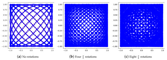
Figure 1. Reducing sampling gaps with rotations. (a) The Lissajous curve (red line) and its sampling (blue dots). Note that the Lissajous curve features gaps which cannot be reduced by just increasing the sampling the rate. Instead, the gaps are reduced by merging samplings of rotated versions of the Lissajous curve. (b,c) The merged sampling with four and eight rotations, respectively.

Extension to Rigid Body Motions and Multi-Patch Sequences. It is straightforward to extend the proposed approach to rigid body motions that also include translations. If the specimen is not only rotated by an angle $\alpha$ but also shifted by an offset b, we obtain scan data $\widehat{s}\left(t\right)$ corresponding to $\widehat{\rho }\left(x\right)=\rho \left(Q_{\alpha }^T(x-b)\right)$. Again, the change of variables $y=Q_{\alpha }^T(x-b)$ yields the relationship to the original $\rho$ by

$$\begin{array}{cc}\hfill \widehat{s}\left(t\right)& =Q_{\alpha }A\left[\rho \right]\left(Q_{\alpha }^T(r\left(t\right)-b)\right)Q_{\alpha }^{T}v\left(t\right),\hfill \end{array}$$

(39)

analogous to Equation (37). Consequently, the reverse operation $(Q_{\alpha }^T{s}_k,Q_{\alpha }^T(r_k-b),Q_{\alpha }^T{v}_k)$ needs to be performed on the data samples before it is merged with that of other scans. We want to point out that this extension can in particular handle data as acquired in so-called multi-patch sequences. Multi-patch sequences combine just translated versions of a standard scan trajectory such as Lissajous curves which are used to enlarge the effective field of view (cf. [13,14]).

5. Numerical Experiments

5.1. Experimental Setup

The algorithms presented in this paper were implemented in Python 3.9, using Numpy, SciPy, and PyTorch. The numerical experiments were performed on a laptop equipped with an Intel Core i7 CPU, 16 GB of RAM, and Windows 10.

Simulation of Data. To obtain simulated MPI scans we proceed as follows: As a base trajectory we use the 2D Lissajous of Equation (38) with the the parameter settings of the Open MPI project [26] and 1632 sample locations. Using this trajectory we simulate 2D scans of phantoms and rotated versions of it. The simulated scan data $s\left(t\right)$ is obtained through Equation (3) with the resolution parameter set to $h=0.01$ (the motivation of this choice is explained in [22]). Moreover, we add $10\%$ Gaussian noise to account for noise in measured data. This means that the discrete simulated scan data is given by

$$\begin{array}{cccc}\hfill s_k& =s\left(t_k\right)+\epsilon N_k,\hfill & \hfill \epsilon & =0.1\underset{k=1,\dots ,L}{max}\left\{|s\left(t_k\right)|\right\},\hfill \end{array}$$

(40)

where $N_k\sim \mathcal{N}(0,1)$ are i.i.d. standard normally distributed random variables.

Reconstruction Grid. For the discrete algorithms in the 2D setup, we fix a grid on the FOV $\mathsf{\Omega }={[-1,1]}^2$. In principle, we may choose any grid for the reconstruction, since the data acquisition, i.e., sampling along the (rotated) trajectories of Figure 1, is not related to this choice. Further note that the errors in the time series of acquired data (and thus also the errors in the corresponding frequency band) are not related to the choice of the spatial grid but to the time sampling. In all our experiments we employ a $N_x\times N_y=100\times 100$ grid on $\mathsf{\Omega }={[-1,1]}^2$. Thus, we have $N=N_x·N_y=$ 10,000 pixels and mesh widths of $h_x=h_y=0.04$. We point out that this choice can be considered a higher resolution setup, because in current practical setups, such as the Open MPI project [26], the usual grid sizes are smaller than $40\times 40$.

Employed Algorithms and Choice of Parameters. In the experiments we employ the two stage scheme described in Section 3. For Stage 1, we use the variational inpainting model of [23] described in Section 3.1. A discussion of the advantages of the variational approach over the LLSq method in [22] can be found in the experimental section of [23]. For Stage 2, we deconvolve in a regularized fashion as defined in Equation (9), with the Tikhonov regularization of Equation (10) and the TV smooth regularization of Equation (11).

Concerning the (hyper-)parameters used in Stage 1, we use the following settings. For the regularization weight $\lambda$ of Equation (8) we set $\lambda =25.0/\mathrm{nRot}$, where $\mathrm{nRot}\in \{1,4,8\}$ represents the number of scans performed (with angles $\frac{2\pi n}{\mathrm{nRot}}$ and $n\in \{0,\dots ,\mathrm{nRot}-1\}$). Further, we use a maximum number of 1000 CG iterations if a tolerance of $5\times {10}^{-12}$ is not reached before. In Stage 2 with the Tikhonov regularization in Equation (10), we use ${\mu }_{\mathrm{Tik}}=5.125\times {10}^{-4}$ as a regularization weight. The maximum number of CG iterations is 10,000, if a tolerance of $5\times {10}^{-12}$ is not reached. The (hyper-)parameters used in Stage 2 with TV smooth regularization (11), are the following: as a regularization weight we employ ${\mu }_{\mathrm{TV}}=1.825\times {10}^{-3}$. The TV smooth parameter $\delta$, is set to $\delta ={10}^{-16}$. For the fixed point iteration we use a maximum number of 10 iterations.

The tolerance of the CG-solver applied within the fixed point iteration is set to ${10}^{-6}$ and a maximum number of 100,000 CG iterations. In all cases where the CG-solver is employed, the maximum number of CG iterations was set sufficiently large for the solver to stop at the requested tolerance.

Motivation for the Choice of Regularization Parameters. The particular choice of the parameters $\lambda$ of Stage 1 and $\mu$ of Stage 2, for both Tikhonov and TV smooth regularization, were found by manual tuning guided by the PSNR and SSIM scores (defined below). The parameters were then kept fixed throughout all experiments of the paper. We support and motivate our hand-crafted choice by the following more systematic investigation. First, we consider the setup without rotations and isolate Stage 1 to find a suitable parameter $\lambda$. To this end, we convolve the ground truth image $\rho$ with ${\kappa }_h$ to obtain “intermediate ground truth” data ${\kappa }_h\ast \rho$ which is used to compute the PSNR and SSIM scores of the intermediate results $u=trace\left(I\left[A\right]\right)$ of Stage 1; cf. Equation (5). Exemplarily, corresponding PSNR and SSIM curves for Stage 1 obtained with the vessel-shaped phantom are displayed in Figure 2. On the one hand, we observe that the optimal SSIM and PSNR values are significantly different and, on the other hand, that both SSIM and PSNR are rather insensitive to $\lambda$-values in the interval $[15,35]$. The situation is similar for all other experiments of the paper; in particular, we found that the numerical values of the SSIM and the PSNR scores for $\lambda \in [15,35]$ only deviate by at most 5% from the corresponding SSIM and PSNR scores for $\lambda =25$ in all experiments. This motivates our hand-crafted fixed choice $\lambda =25$. Concerning the purpose of the corresponding Stage 1 regularizer, we note that it is responsible for inpainting (gap filling) besides denoising. Thus, $\lambda$ depends on the spatial density of the sampling locations. In the case of rotations, a denser sampling of the FOV is provided (cf. Figure 1) and therefore smaller parameter values as a function of the number of rotations are reasonable. Based on the reference value $\lambda =25$ (from the case without rotations) the parameter value is reduced according to ${\lambda }_{\mathrm{nRot}}=\lambda ·f\left(\mathrm{nRot}\right)$ with a decreasing function $f\left(\mathrm{nRot}\right)$. Here, we chose the particular (simple) function $f\left(\mathrm{nRot}\right)=1/\mathrm{nRot}$.

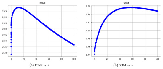
Figure 2. Motivation for the choice of the Stage 1 regularization parameter $\lambda$. (a,b) show the PSNR and SSIM as functions of $\lambda$. The curves here were obtained from the vessel-shaped phantom. Both SSIM and PSNR are rather insensitive to $\lambda$-values in the interval $[15,35]$, which contains our particular choice $\lambda =25$.

Next we consider the parameter $\mu$ of Stage 2. Again, we look at the setup without rotations and the parameter $\lambda$ of Stage 1 kept fixed at $\lambda =25$. Exemplarily, for the vessel-shaped phantom, PSNR values after Stage 2 for both Tikhonov and TV-smooth regularization are displayed in Figure 3 as functions of $log\left(\mu \right)$. We observe that our parameter choices for ${\mu }_{\mathrm{Tik}}$ and ${\mu }_{\mathrm{TV}}$ are rather close to the optimal PSNR values (which are however rather different to optimal SSIM values as observed for Stage 1 as well). Again, the situation is similar in all other experiments of the paper, which motivates our fixed choice for all experiments.

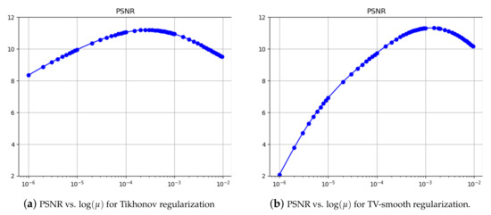
Figure 3. Motivation for the choice of the Stage 2 regularization parameters $\mu$. (a,b) show the PSNR as functions of $log\left(\mu \right)$ for Tikhonov and TV-smooth regularization, respectively. The curves were obtained from the vessel-shaped phantom keeping the Stage 1 parameter fixed at $\lambda =25$. Our particular choices, which are ${\mu }_{\mathrm{Tik}}=5.125\times {10}^{-4}$ with respect to Tikhonov regularization and ${\mu }_{\mathrm{TV}}=1.825\times {10}^{-3}$ with respect to TV-smooth regularization, are very close to the optimal values.

Quantitative Assessment. For the quantitative assessment of the quality of reconstructions we compute both the Peak Signal-to-Noise Ratio (PSNR) and the Structural Similarity Index Measure (SSIM). For a pair of images ${\rho }_{\mathrm{GT}}$ (the ground truth) and a reconstruction ${\rho }_{\mathrm{rec}}\in \{{\rho }_{\mathrm{Tik}},{\rho }_{\mathrm{TV}}\}$, the PSNR is defined as follows:

$$\begin{array}{cc}\hfill \mathrm{PSNR}& =10{log}_{10}\left(\frac{max{\rho }_{\mathrm{GT}}^2}{\mathrm{MSE}}\right)\hfill \end{array}$$

(41)

where ${\displaystyle \mathrm{MSE}=\frac{1}{N_x{N}_y}\sum _{i=0}^{N_x-1}\sum _{j=0}^{N_y-1}{\left({\rho }_{\mathrm{GT},i,j}-{\rho }_{\mathrm{rec},i,j}\right)}^2}$ denotes the Mean Square Error, and ${\rho }_{\mathrm{GT},i,j}$, ${\rho }_{\mathrm{rec},i,j}$ are the $(i,j)$-th pixel of the images. The definition of SSIM is technically significantly more involved. Therefore, we refer the reader to [32] for a thorough introduction to SSIM.

5.2. Experimental Results

Experiment 1. In our first experiment (cf. Figure 4a), we consider a simple-structured phantom with different concentration levels for which we use the term concentration phantom. More specifically, we chose relative concentration levels of 1, $0.75$, $0.5$, and $0.25$. We consider reconstruction using the model-based two stage approach using regularized deconvolution via Equation (9) with Tikhonov regularization (10) and TV smooth regularization (11) for Stage 2. We compare the algorithms for different numbers of rotated scan trajectories: concretely, we consider sequences of $n=1,4,8$ trajectories with corresponding rotation angles being multiples of $\frac{2\pi }{n}.$

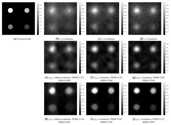
Figure 4. Reconstruction of different concentration levels using model-based two-stage reconstruction for combining rotated scan trajectories. The ground truth consists of four circular regions with decreasing (relative) concentrations levels: 1, $0.75$, $0.5$, and $0.25$. First row. Trace fields $u=traceA\left[\rho \right]$ (output of Stage 1) obtained with increasing number of rotations $0,4,8.$ Second row. Reconstruction results ${\rho }_{\mathrm{Tik}}$ using Tikhonov regularized deconvolution in Stage 2 with increasing number of rotations. Third row. Reconstruction results ${\rho }_{\mathrm{TV}}$ using TV smooth regularized deconvolution in Stage 2 with increasing number of rotations. We observe qualitatively and quantitatively increasing reconstruction quality with increasing number of merged rotated scans for both Tikhonov and TV type regularization. Further, the TV smooth regularized deconvolution in Stage 2 is capable of reconstructing the edges while the Tikhonov regularized deconvolution in Stage 2 smoothes the edges.

We observe qualitatively increasing reconstruction quality with increasing number of merged rotated scans for both Tikhonov and TV type regularization. Further, the experiment qualitatively confirms the common observation that the TV type reconstruction is capable of reconstructing the edges while the Tikhonov reconstruction smooths them out.

From a physical viewpoint it is reasonable to assume that the amount of tracer does not change while flowing in the specimen. Mathematically, this translates to the desired property that a reconstruction scheme should reproduce the total concentration as good as possible. We experimentally investigate this property here by comparing the total concentration of the ground truth with that produced by the reconstruction schemes (cf. Table 1). We employed the following preprocessing: if a pixel value is negative, we set it to zero (which is reasonable since concentrations are nonnegative quantities.) From Table 1 we infer that the two stage reconstruction scheme using TV-smooth regularization in Stage 2 preserves the concentration rather well.

Table 1. Preservation of the concentration in Experiment 1.

nRot	Total Concentration of the Ground Truth	Total Concentration, Tikhonov Reconstruction in Stage 2	Total Concentration, TV Smooth Reconstruction in Stage 2
1	0.177	0.191236	0.181551
4	0.177	0.203939	0.178848
8	0.177	0.202336	0.178237

Experiment 2. In our second experiment (cf. Figure 5), we consider a more complex angular ring or O-shaped structure. We investigate the effect of decreasing the size of the object to see the limits of the considered model-based two stage approach using regularized deconvolution via Equation (9) with Tikhonov regularization (10) and TV smooth regularization (11) for Stage 2. We again compare the algorithms for the combination of scan sequences of $n=1,4,8$ trajectories with corresponding rotation angles being multiples of $\frac{2\pi }{n}.$

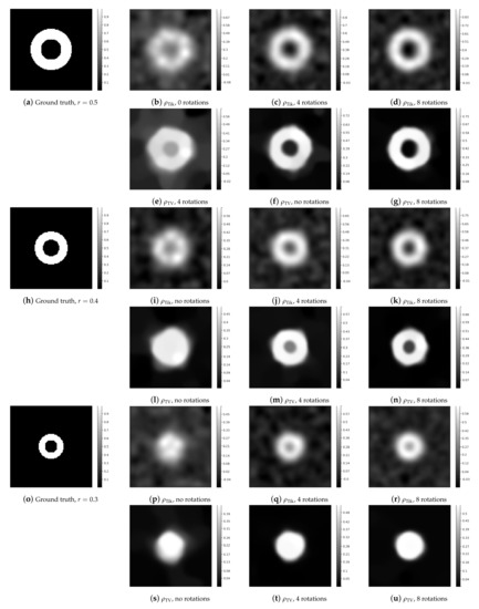
Figure 5. Effect of decreasing the size of the object. The ground truth consists of circular rings of decreasing size. First row. Trace fields $u=traceA\left[\rho \right]$ (output of Stage 1) obtained with increasing number of rotations $0,4,8.$ Second and third row. Reconstruction results ${\rho }_{\mathrm{Tik}}$ using Tikhonov (second row) and TV smooth (third row) regularized deconvolution in Stage 2 with increasing number of rotations. We observe qualitatively increasing reconstruction quality with increasing number of rotated scans for both deconvolution schemes. The scheme using Tikhonov regularized deconvolution smoothes the edges; in the case of no rotations, it becomes hard to visually recognize the ring-shape when diminishing the size; with increasing number of rotations, the ring shape is reconstructed even for a small ring size. The scheme using TV smooth regularized deconvolution better preserves the edges; for a large ring size, one may very well infer on the object from the reconstructions; for smaller ring sizes the outer object boundary still remains rather sharp, but the inner hole is no longer reconstructed.

As in Experiment 1, we observe qualitatively increasing reconstruction quality with increasing number of merged rotated scans for both regularized deconvolution schemes. We further observe that the scheme using Tikhonov regularized deconvolution smooths the edges. In particular, in the case of a single scan (no rotations), it is hard to visually recognize the ring-shape when diminishing the size of the ring phantom. However, with an increasing number of rotations, the ring shape is reconstructed even for a small size of the ring phantom. The scheme using TV smooth regularized deconvolution better preserves the edges. Further, for a large ring size, one may very well infer the shape of the object from the reconstruction. Notably, we mention that the reconstruction from 8 angular scans in Figure 5g visually almost equals the ground truth. For smaller ring sizes the outer object boundary still remains rather sharp, but the inner hole is no longer reconstructed depending on the number of rotational scans—the more scans the smaller the size of the phantom may be to still reconstruct the angular ring structure.

Experiment 3. In our third experiment (cf. Figure 6) we study a more realistic vessel-shaped phantom. The phantom is designed to mimic in particular the junctions of blood vessels. In the left column of Figure 6, one can see that already with no rotations the basic structure emerges. By merging $n=4$ (middle column) or $n=8$ (right column) rotated scans (with corresponding rotation angles $\frac{2\pi j}{n}$ for $j\in \{0,\dots ,n-1\}$), we obtain a clearer picture of the structure and the locations of junctions become more distinctive. We observe that using the merging of rotational scans as opposed to not doing so enhances the quality of the reconstructions for both Tikhonov and TV-smooth type regularization. This manifests also in terms of the two employed quality measures which are the Peak Signal-to-Noise Ratio (PSNR) and the Structural Similarity Index Method (SSIM).

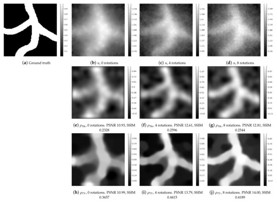
Figure 6. Reconstruction of a vessel-shaped phantom using model-based two-stage reconstruction for combining rotated scan trajectories. First row. Trace fields $u=traceA\left[\rho \right]$ (output of Stage 1) obtained with increasing number of rotations $0,4,8$. Second row. Reconstruction results ${\rho }_{\mathrm{Tik}}$ using Tikhonov regularized deconvolution in Stage 2 with increasing number of rotations. Third row. Reconstruction results ${\rho }_{\mathrm{TV}}$ using TV smooth regularized deconvolution in Stage 2 with increasing number of rotations. We observe qualitatively in the case of a more realistic phantom that merging rotated scans helps to enhance the quality of the reconstruction for both Tikhonov and TV type regularization. In particular, the locations of junctions become more distinctive with rotations.

Experiment 4. In the fourth experiment (cf. Figure 7), we consider a vessel-shaped phantom which features more and finer structures. While in Experiment 3 the branches of the vessels have almost uniform thickness, the thickness here varies more and vessels become even thinner than the O-shape of Experiment 2. For the results displayed in Figure 7, we merge again $n=1$ (left column), $n=4$ (middle column) or $n=8$ (right column) rotated scans (with corresponding angles $\frac{2\pi j}{n}$ for $j\in \{0,\dots ,n-1\}$) and employ Tikhonov regularization (second row) as well as TV smooth regularization (third row) in the deconvolution Stage 2. As in Experiment 3, we observe that using rotations as opposed to no rotations enhances again the quality of the reconstructions for both Tikhonov and TV-smooth type regularization, qualitatively and in terms of PSNR or SSIM. All locations of junctions become more distinctive with rotations. We observe here, too, as in Experiment 2, that finer structures of smaller scale are more difficult to reconstruct. The finer structures have apparently less contrast in all the reconstructions but still become better perceptible when rotated scans are combined.

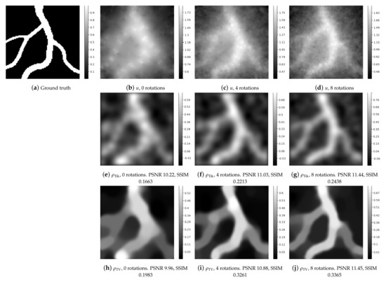
Figure 7. Reconstruction of a vessel-shaped phantom with finer structures using model-based two-stage reconstruction for combining rotated scan trajectories. First row. Trace fields $u=traceA\left[\rho \right]$ (output of Stage 1) obtained with increasing number of rotations $0,4,8$. Second row. Reconstruction results ${\rho }_{\mathrm{Tik}}$ using Tikhonov regularized deconvolution in Stage 2 with increasing number of rotations. Third row. Reconstruction results ${\rho }_{\mathrm{TV}}$ using TV smooth regularized deconvolution in Stage 2 with increasing number of rotations. We observe qualitatively that again merging rotated scans helps to enhance the quality of the reconstruction for both Tikhonov and TV type regularization. In particular, the locations of junctions become more distinctive with rotations. We observe here too, that finer structures of smaller scale are generally more difficult to reconstruct but still become better perceptible when rotated scans are combined.

Experiment 5. In the fifth experiment (cf. Figure 8), we consider non piecewise constant data (in contrast to the previous experiments where the ground truth was either binary or piecewise constant). As a ground truth we consider the indicator function of an rectangle with four-to-three aspect ratio which we convolved with a Gaussian kernel with variance parameter corresponding to a tenth of the image size; see Figure 8a. As in the previous experiments for piecewise constant data, we observe that using rotations as opposed to no rotations enhances the quality of the reconstructions for both Tikhonov and TV-smooth type regularization, qualitatively and in terms of PSNR and SSIM. Further, the TV reconstructions show the well-known staircasing effect, i.e., constant plateaus are introduced in the respective reconstruction.

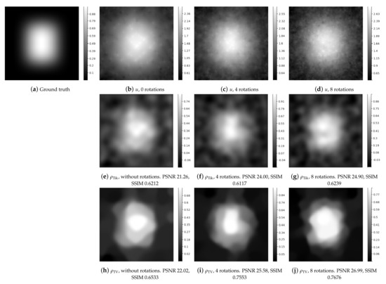
Figure 8. Reconstruction of smoothed rectangle (convolution with a Gaussian with $\sigma$ of $1/10$ of the image size) using model-based two-stage reconstruction for combining rotated scan trajectories. First row. Trace fields $u=traceA\left[\rho \right]$ (output of Stage 1) obtained with increasing number of rotations $0,4,8.$ Second row. Reconstruction results ${\rho }_{\mathrm{Tik}}$ using Tikhonov regularized deconvolution in Stage 2 with increasing number of rotations. Third row. Reconstruction results ${\rho }_{\mathrm{TV}}$ using TV smooth regularized deconvolution in Stage 2 with increasing number of rotations. We observe qualitatively and quantitatively increasing reconstruction quality with increasing number of merged rotated scans for both Tikhonov and TV type regularization. The TV smooth regularized deconvolution results in Stage 2 exhibit the well-known staircasing effect.

A summary of the quantitative reconstruction results is provided in Table 2. We observe that this summary underpins the finding that an increasing number of rotations quantitatively increases the reconstruction quality for both Tikhonov and TV type regularization.

Table 2. Summary of the PSNR and SSIM scores of all experiments.

	nRot	Tikhonov		TV Smooth
		PSNR	SSIM	PSNR	SSIM
Figure 4	1	17.57	0.4285	17.34	0.4293
	4	19.37	0.5249	19.97	0.7190
	8	19.97	0.5764	21.21	0.7853
Figure 5a	1	12.85	0.2238	12.84	0.2933
	4	14.88	0.3303	15.61	0.5964
	8	15.84	0.3764	17.26	0.7256
Figure 5h	1	14.08	0.3358	13.75	0.4886
	4	15.53	0.3894	15.58	0.6891
	8	16.15	0.4071	16.68	0.7931
Figure 5o	1	15.52	0.4314	15.82	0.5516
	4	16.70	0.4650	16.53	0.8134
	8	16.98	0.4977	16.87	0.8179
Figure 6	1	10.93	0.2328	10.99	0.3657
	4	12.61	0.2596	13.79	0.4415
	8	12.81	0.2544	14.00	0.4189
Figure 7	1	10.22	0.1663	9.96	0.1983
	4	11.03	0.2213	10.88	0.3261
	8	11.44	0.2438	11.45	0.3365
Figure 8	1	21.26	0.6212	22.02	0.6533
	4	24.00	0.6117	25.58	0.7553
	8	24.90	0.6239	26.99	0.7676

6. Discussion

As a first contribution of the paper, we have extended the algorithmic framework of [22] by a TV-smooth regularization in Stage 2. This complements [23], whose focus was the variational inpainting-type reconstruction of Stage 1 and which resulted in an overall enhanced and more flexible method. In particular, we are now able to process data from scan trajectories which are as sparse as those employed in the Open MPI project [26]. Secondly, we have developed a model-based reconstruction scheme for quality-enhancement by the combination of scans along multiple trajectories. Basing on the reconstruction model’s independence of the particular scan trajectories and the algorithmic framework’s independence of any temporal causality we were able to process the data as a point cloud in extended phase space. More precisely, we transformed the collected data from different scan trajectories to point cloud data in extended phase space, and employed our model-based reconstruction schemes to enhance the quality of reconstructions. In particular, we worked out the case of rotated scan trajectories. We point out that different trajectories may be obtained via simple geometric transformations such as translations and rotations including so-called multi-patch scan sequences as a special case. Finally, we have conducted numerical experiments using simulated data to demonstrate the proposed technique’s potential.

Topics of future research include improving the variational inpainting scheme used for Stage 1 of the considered two-stage reconstruction process (cf. the small peaks visible in the reconstruction of the trace fields; cf., e.g., Figure 6) as well as considering in more detail the multi-patch setups mentioned. Further, the investigation of automatic parameter choice rules for both parameters are an important topic of future research.

7. Conclusions

To conclude, in this paper we have proposed a quality-enhancing technique based on the combination of multiple trajectories using model-based reconstruction. We have illustrated the benefits of the proposed quality-enhancing technique by numerical experiments. As a consequence of our simulation study we want to suggest to experimenters to rotate the specimen in the MPI scanner with respect to four angles, i.e., $0,90,180,$ and 270 degrees, and to repeat the same scanning process under these rotations. This does not require changing the settings of the MPI scanner, and is precisely the information needed for the proposed method.

References

- Gleich, B.; Weizenecker, J. Tomographic imaging using the nonlinear response of magnetic particles. Nature 2005, 435, 1214–1217. [Google Scholar] [CrossRef] [PubMed]
- Knopp, T.; Buzug, T.M. Magnetic Particle Imaging: An Introduction to Imaging Principles and Scanner Instrumentation; Springer: Berlin/Heidelberg, Germany, 2012. [Google Scholar]
- Zheng, B.; Vazin, T.; Yang, W.; Goodwill, P.; Saritas, E.; Croft, L.; Schaffer, D.; Conolly, S. Quantitative stem cell imaging with magnetic particle imaging. In Proceedings of the IEEE International Workshop on Magnetic Particle Imaging, Berkeley, CA, USA, 23–24 March 2013; p. 1. [Google Scholar]
- Graeser, M.; Thieben, F.; Szwargulski, P.; Werner, F.; Gdaniec, N.; Boberg, M.; Griese, F.; Möddel, M.; Ludewig, P.; van de Ven, D.; et al. Human-sized magnetic particle imaging for brain applications. Nat. Commun. 2019, 10, 1936. [Google Scholar] [CrossRef] [PubMed]
- Ter-Pogossian, M.; Phelps, M.; Hoffman, E.; Mullani, N. A positron-emission transaxial tomograph for nuclear imaging (PETT). Radiology 1975, 114, 89–98. [Google Scholar] [CrossRef] [PubMed]
- Kuhl, D.; Edwards, R. Image separation radioisotope scanning. Radiology 1963, 80, 653–662. [Google Scholar] [CrossRef]
- Knopp, T.; Biederer, S.; Sattel, T.; Erbe, M.; Buzug, T. Prediction of the spatial resolution of magnetic particle imaging using the modulation transfer function of the imaging process. IEEE Trans. Med. Imaging 2011, 30, 1284–1292. [Google Scholar] [CrossRef]
- Weizenecker, J.; Borgert, J.; Gleich, B. A simulation study on the resolution and sensitivity of Magnetic Particle Imaging. Phys. Med. Biol. 2007, 52, 6363–6374. [Google Scholar] [CrossRef]
- Rahmer, J.; Weizenecker, J.; Gleich, B.; Borgert, J. Analysis of a 3-D system function measured for Magnetic Particle Imaging. IEEE Trans. Med. Imaging 2012, 31, 1289–1299. [Google Scholar] [CrossRef]
- Lampe, J.; Bassoy, C.; Rahmer, J.; Weizenecker, J.; Voss, H.; Gleich, B.; Borgert, J. Fast reconstruction in Magnetic Particle Imaging. Phys. Med. Biol. 2012, 57, 1113–1134. [Google Scholar] [CrossRef]
- Knopp, T.; Rahmer, J.; Sattel, T.; Biederer, S.; Weizenecker, J.; Gleich, B.; Borgert, J.; Buzug, T. Weighted iterative reconstruction for magnetic particle imaging. Phys. Med. Biol. 2010, 55, 1577–1589. [Google Scholar] [CrossRef]
- Storath, M.; Brandt, C.; Hofmann, M.; Knopp, T.; Salamon, J.; Weber, A.; Weinmann, A. Edge preserving and noise reducing reconstruction for Magnetic Particle Imaging. IEEE Trans. Med. Imaging 2016, 36, 74–85. [Google Scholar] [CrossRef]
- Szwargulski, P.; Möddel, M.; Gdaniec, N.; Knopp, T. Efficient joint image reconstruction of multi-patch data reusing a single system matrix in magnetic particle imaging. IEEE Trans. Med. Imaging 2018, 38, 932–944. [Google Scholar] [CrossRef] [PubMed]
- Gdaniec, N.; Boberg, M.; Möddel, M.; Szwargulski, P.; Knopp, T. Suppression of motion artifacts caused by temporally recurring tracer distributions in multi-patch magnetic particle imaging. IEEE Trans. Med. Imaging 2020, 39, 3548–3558. [Google Scholar] [CrossRef] [PubMed]
- Rahmer, J.; Weizenecker, J.; Gleich, B.; Borgert, J. Signal encoding in Magnetic Particle Imaging: Properties of the system function. BMC Med. Imaging 2009, 9, 4. [Google Scholar] [CrossRef] [PubMed]
- Knopp, T.; Sattel, T.F.; Biederer, S.; Rahmer, J.; Weizenecker, J.; Gleich, B.; Borgert, J.; Buzug, T.M. Model-Based Reconstruction for Magnetic Particle Imaging. IEEE Trans. Med. Imaging 2010, 29, 12–18. [Google Scholar] [CrossRef] [PubMed]
- Schomberg, H. Magnetic Particle Imaging: Model and reconstruction. In Proceedings of the 2010 IEEE International Symposium on Biomedical Imaging: From Nano to Macro, Rotterdam, The Netherlands, 14–17 April 2010; pp. 992–995. [Google Scholar]
- Goodwill, P.; Conolly, S.M. The X-Space Formulation of the Magnetic Particle Imaging Process: 1-D Signal, Resolution, Bandwidth, SNR, SAR, and Magnetostimulation. IEEE Trans. Med. Imaging 2010, 29, 1851–1859. [Google Scholar] [CrossRef] [PubMed]
- Goodwill, P.; Conolly, S.M. Multidimensional X-Space Magnetic Particle Imaging. IEEE Trans. Med. Imaging 2011, 30, 1581–1590. [Google Scholar] [CrossRef] [PubMed]
- Grüttner, M.; Knopp, T.; Franke, J.; Heidenreich, M.; Rahmer, J.; Halkola, A.; Kaethner, C.; Borgert, J.; Buzug, T.M. On the Formulation of the Image Reconstruction Problem in Magnetic Particle Imaging. Biomed. Eng. 2013, 58, 583–591. [Google Scholar] [CrossRef]
- Bringout, G.; Erb, W.; Frikel, J. A new 3D model for magnetic particle imaging using realistic magnetic field topologies for algebraic reconstruction. Inverse Probl. 2020, 36, 124002. [Google Scholar] [CrossRef]
- März, T.; Weinmann, A. Model-based reconstruction for Magnetic Particle Imaging in 2D and 3D. Inverse Probl. Imaging 2016, 10, 1087–1110. [Google Scholar] [CrossRef]
- März, T.; Gapyak, V.; Weinmann, A. A two-stage Model-Based Regularized Reconstruction Approach for Magnetic Particle Imaging. In Proceedings of the AIP Conference Proceedings; AIP Publishing LLC: Melville, NY, USA, submitted.
- Bertero, M.; Boccacci, P.; De Mol, C. Introduction to Inverse Problems in Imaging; CRC Press: Boca Raton, FL, USA, 2021. [Google Scholar]
- Kirsch, A. An Introduction to the Mathematical Theory of Inverse Problems; Springer: Berlin/Heidelberg, Germany, 2011; Volume 120. [Google Scholar]
- Knopp, T.; Szwargulski, P.; Griese, F.; Gräser, M. OpenMPIData: An initiative for freely accessible Magnetic Particle Imaging data. Data Brief 2020, 28, 104971. [Google Scholar] [CrossRef]
- Chikazumi, S.; Charap, S. Physics of Magnetism; Krieger Publishing: New York, NY, USA, 1978. [Google Scholar]
- Jiles, D. Introduction to Magnetism and Magnetic Materials; CRC Press: Boca Raton, FL, USA, 1998. [Google Scholar]
- Vogel, C.R.; Oman, M.E. Iterative methods for total variation denoising. SIAM J. Sci. Comput. 1996, 17, 227–238. [Google Scholar] [CrossRef]
- Vogel, C.R.; Oman, M.E. Fast, robust total variation-based reconstruction of noisy, blurred images. IEEE Trans. Image Process. 1998, 7, 813–824. [Google Scholar] [CrossRef] [PubMed]
- Golub, G.H.; Van Loan, C.F. Matrix Computations; JHU Press: Baltimore, MD, USA, 2013. [Google Scholar]
- Wang, Z.; Bovik, A.C.; Sheikh, H.R.; Simoncelli, E.P. Image quality assessment: From error visibility to structural similarity. IEEE Trans. Image Process. 2004, 13, 600–612. [Google Scholar] [CrossRef] [PubMed] [Green Version]
Publisher’s Note: MDPI stays neutral with regard to jurisdictional claims in published maps and institutional affiliations. |
© 2022 by the authors. Licensee MDPI, Basel, Switzerland. This article is an open access article distributed under the terms and conditions of the Creative Commons Attribution (CC BY) license (https://creativecommons.org/licenses/by/4.0/).