Boundary Value Problem of Space-Time Fractional Advection Diffusion Equation

Abstract

In this article, the analytical and numerical solution of a one-dimensional space-time fractional advection diffusion equation is presented. The separation of variables method is used to carry out the analytical solution, the basis of the system eigenfunction and their corresponding eigenvalue for basic equation is determined, and the numerical solution is based on constructing the Crank-Nicolson finite difference scheme of the equivalent partial integro-differential equations. The convergence and unconditional stability of the solution are investigated. Finally, the numerical and analytical experiments are given to verify the theoretical analysis.

1. Introduction

Recently, interest in the topics of fractional calculus has increased [1]. These topics are used by many scientists to simulate a variety of physical, biological, and chemical processes [2,3]. The space-time fractional advection diffusion equation (STFADE) considers a famous model for anomalous diffusion in several practical fields, such as the diffusion processes of pollutants in porous media and the continuous-time random walk. In [4,5], Gorenflo, Mainardi and Luchko developed discrete random walk models and found that the fundamental solution may be regarded as the probability density of a self-similar random process evolving in time, which can be viewed as a generalized diffusion process.

The use of fractional derivatives (FDs) for modeling real physical processes or environments leads to the appearance of equations containing derivatives and integrals of fractional order in addition to the classical ones. Researchers have focused their efforts on fractional-order physical models of non-equilibrium processes [6,7]. As a result, they study the linear elasticity and viscoelastic deformation processes in biomaterials and capillary-porous materials with fractal structures. Recent applications of fractional equations to many biological systems are more adequate than the previously used integer-order biological systems, because fractional-order derivatives and integrals describe the memory and hereditary properties of different substances [8,9,10,11,12].

This paper is concerned with methods for obtaining accurate numerical and analytical approximations to the solutions of fractional sub-diffusion equations (the ultra-slow diffusion model with time fractional derivative $0<\alpha <1$), which is even more slow than the power-law sub-diffusion and is widely observed in a variety of natural and engineering fields. In this paper, we investigate the one-dimensional STFADE with the source term

$$\begin{array}{cc}\hfill \frac{{\partial }^{\alpha }z(\rho ,t)}{\partial t^{\alpha }}& {=}_0^R{D}_{\rho }^{\beta }z(\rho ,t)+s(\rho ,t),\hfill \\ \hfill z(0,t)& =z(1,t)=0,0<t<T,\hfill \\ \hfill z(\rho ,0)& =\varphi \left(\rho \right),0<\rho <1,\hfill \end{array}$$

(1)

in domain $\omega =(0,1)\times (0,T), 0<T<\infty$, where $0<\alpha <1$ is a parameter describing the order of the fractional derivative in the time direction, and $1<\beta <2$ describes the order of the fractional derivative space direction. ${\displaystyle \frac{{\partial }^{\alpha }z(\rho ,t)}{\partial t^{\alpha }}}$ is the Caputo fractional derivative of order $\alpha$, which is defined by

$$\frac{{\partial }^{\alpha }z(\rho ,t)}{\partial t^{\alpha }}=\left\{\begin{array}{cc}\frac{1}{\Gamma (1-\alpha )}{\int }_0^t{(t-\sigma )}^{-\alpha }\frac{\partial z(\rho ,\sigma )}{\partial \sigma }d\sigma ,\hfill & 0<\alpha <1,0<\sigma <t\hfill \\ \frac{\partial z(\rho ,t)}{\partial t}\hfill & \alpha =1,\hfill \end{array}\right.$$

(2)

and the space fractional derivative $D_{\rho }^{\beta }$ is the Riemann–Liouville fractional derivative operator of order $\beta$ defined by

$$D_{\rho }^{\beta }z(\rho ,t)=\left\{\begin{array}{cc}\frac{1}{\Gamma (2-\beta )}{\displaystyle \frac{d^2}{d{\rho }^2}}{\int }_0^{\rho }{(\rho -\sigma )}^{1-\beta }z(\sigma ,t)d\sigma ,\hfill & 1<\beta <2,0<\sigma <\rho \hfill \\ \frac{{\partial }^{2}z(\rho ,t)}{\partial {\rho }^2}\hfill & \beta =2.\hfill \end{array}\right.$$

(3)

Equation (1) yields the following forms of diffusion equations for various values of the parameters $\alpha$ and $\beta$:

For $\alpha =1$ and $\beta =2$⟶ the classical diffusion equation;

For $0<\alpha <1$ and $\beta =2$ ⟶ the time-fractional diffusion equation;

For $\alpha =1$ and $0<\beta <2$⟶ the space-fractional diffusion equation,

For $0<\alpha <1$ and $0<\beta <2$⟶ the space-time fractional diffusion equation.

This work establishes the fundamental analytical and numerical solution of (1), which is a very general form of STFADE, and many problems that are already studied are special cases of it, as in [13,14,15].

The structure of the paper is organized as follows. In Section 2, some theoretical definitions and proprieties of fractional differentiable classes and Mittage–Leffler functions are presented. In Section 3, we discuss the analytical solution of (1) with the separation of variable method and construct the base system of eigenfunctions and their corresponding eigenvalues of the basic equation. In Section 4 and Section 5, the numerical scheme for solving TSFADE and their convergence and unconditional stability analysis are established. Finally, in Section 6, the numerical experiments are presented.

2. Theoretical Preliminaries

Definition 1

([16]). A real-valued function $\mathsf{\Psi }\left(\tau \right)$ can be said to belong to space $C_{\alpha }[0,\infty ], \alpha \in \mathrm{I}\mathrm{R}$ if there exists a real number $q>\alpha$ such that $\mathsf{\Psi }\left(\tau \right)={\tau }^q\tilde{\mathsf{\Psi }}\left(\tau \right),\tilde{\mathsf{\Psi }}\left(\tau \right)\in C[0,\infty ].$

Definition 2

([16]). A real valued function $\mathsf{\Psi }\left(\tau \right)$ can be said to belong to space $C_{\alpha }^m[0,\infty ], \alpha \in \mathrm{I}\mathrm{R}, m\in \mathrm{I}\mathrm{N}\cup \left\{0\right\}$ if ${\mathsf{\Psi }}^m\in C_{\alpha }[0,\infty ]$.

Definition 3

([17]). Let $E_{\alpha ,\beta }\left(w\right)$ be the two-parameter Mittage–Leffler function on w defined by

$$E_{\alpha ,\beta }\left(w\right)=\sum _{k=0}^{\infty }\frac{w^k}{\Gamma (\alpha k+\beta )},Re\left(\alpha \right)>0,w,\beta \in \mathbb{C}.$$

As an example, it is easy to deduce that the two-parameter Mittag–Leffler function $E_{\alpha ,\beta }\left(w\right)$ is a generalization of the exponential function ($E_{1,1}\left(w\right)=exp\left(w\right)$), hyperbolic functions ($E_{2,1}\left(w^2\right)=cosh\left(w\right)$) and trigonometric functions ($E_{2,2}(-w^2)=sin\left(w\right)/w,E_{2,1}(-w^2)$$=cos\left(w\right)$).

The validity of the following relationships on $E_{\alpha ,\beta }\left(w\right)$ can be easily tested [15]:

1.

$$\begin{array}{cc}\hfill {\int }_0^t& {\sigma }^{\alpha -1}{E}_{\alpha ,\alpha }(-\lambda {\sigma }^{\alpha }){(t-\sigma )}^{\beta -1}{E}_{\alpha ,\beta }(-\mu {(t-\sigma )}^{\alpha })d\sigma \hfill \\ \hfill & =\left\{\begin{array}{cc}{t}^{\beta -1}\frac{E_{\alpha ,\beta }(-\mu t^{\alpha })-E_{\alpha ,\beta }(-\lambda t^{\alpha })}{\lambda -\mu },\hfill & \lambda \ne \mu \hfill \\ t^{\alpha +\beta -1}(\frac{1}{\alpha }{E}_{\alpha ,\alpha +\beta -1}(-\lambda t^{\alpha })+\left(\frac{1-\beta }{\alpha }\right)E_{\alpha ,\alpha +\beta }(-\lambda t^{\alpha }))\hfill & \lambda =\mu ,\hfill \end{array}\right.\hfill \end{array}$$

(4)

2.

$${\int }_0^t{(t-\tau )}^{\rho -1}{\tau }^{\beta -1}{E}_{\alpha ,\beta }\left(\lambda {\tau }^{\alpha }\right)d\tau =\Gamma \left(\rho \right)t^{\rho +\beta -1}{E}_{\alpha ,\beta +\rho }\left(\lambda t^{\alpha }\right)$$

(5)

Lemma 1

([16]). If $\alpha <2,\beta \in \mathbb{R},\theta$ is such that $\pi \alpha /2<\theta <min(\pi ,\pi \alpha ),w\in \mathbb{C}$ such that $\left|w\right|\ge 0,\theta \le |arg(w\left)\right|\le \pi$; then

$$|E_{\alpha ,\beta }\left(w\right)|\le \frac{C}{1+\left|w\right|}$$

3. Analytical Solution of STFADE

In this section, we proceed with a discussion of the theorem of the existence of aa solution of the boundary value problem for Equation (1) by using the separation of variables method (Fourier method).

Theorem 1.

For every $s(\rho ,t)\in C_{\alpha ,\beta }^{\left(1\right),\left(2\right)}\left(\omega \right)$ and $\varphi \left(\rho \right)\in C(0,1)$, the regular solution $z(\rho ,t)\in C_{\alpha ,\beta }^{\left(1\right),\left(2\right)}\left(\omega \right)$ of the boundary value problems 1 can be represented in the form

$$z(\rho ,t)=\sum _{m=1}^{\infty }\left({\varphi }_m{E}_{\alpha ,1}(-{\lambda }_m{t}^{\alpha })+{\int }_0^t{\tau }^{\alpha -1}{E}_{\alpha ,\alpha }(-{\lambda }_m{\tau }^{\alpha })s_m(t-\tau )d\tau \right){\rho }^{\beta -1}{E}_{\beta ,\beta }(-{\lambda }_m{\rho }^{\beta }).$$

(6)

Here, $E_{\alpha ,\beta }\left(z\right)$-is the well-known function of two parameters of the Mittag–Leffler type: ${\varphi }_m,s_m\left(t\right)$ —the decomposition coefficients of functions $\varphi \left(\rho \right)$ and $s(\rho ,t)$, respectively, on the basis of functions $P_m(\rho ,{\lambda }_m)={\rho }^{\beta -1}{E}_{\beta ,\beta }\left({\lambda }_m{\rho }^{\beta }\right)$.

To solve the boundary value problem (1), we represent the function $z(\rho ,t)$ in the form

$$z(\rho ,t)=z_1(\rho ,t)+z_2(\rho ,t)$$

(7)

According to (7), the boundary value problem (1) can be divided into two boundary value problems as follows:

$$\begin{array}{cc}\hfill \frac{{\partial }^{\alpha }{z}_1(\rho ,t)}{\partial t^{\alpha }}& {=}_0^R{D}_{\rho }^{\beta }{z}_1(\rho ,t),\hfill \\ \hfill z_1(0,t)& =z_1(1,t)=0,0<t<T,\hfill \\ \hfill z_1(\rho ,0)& =\varphi \left(\rho \right),0<\rho <1,\hfill \end{array}$$

(8)

and

$$\begin{array}{cc}\hfill \frac{{\partial }^{\alpha }{z}_2(\rho ,t)}{\partial t^{\alpha }}& {=}_0^R{D}_{\rho }^{\beta }{z}_2(\rho ,t)+s(\rho ,t),\hfill \\ \hfill z_2(0,t)& =z_2(1,t)=0,0<t<T,\hfill \\ \hfill z_2(\rho ,0)& =0,0<\rho <1.\hfill \end{array}$$

(9)

In general, as is customary in solving such problems by the Fourier method, we first consider the homogeneous fractional partial differential Equation (8). The essence of this problem is to find a non-trivial solution represented as product $z_1=P\left(\rho \right)T\left(t\right)$; therefore, Equation (8) can be valid in the case

$$\frac{{}^c{D}_t^{\alpha }T\left(t\right)}{T\left(t\right)}=\frac{{}^R{D}_{\rho }^{\beta }P\left(\rho \right)}{P\left(\rho \right)}=-\lambda ,$$

Then, we can obtain the following fractional differential equations:

$${}^R{D}_{\rho }^{\beta }P\left(\rho \right)+\lambda P\left(\rho \right)=0,P\left(0\right)=P\left(1\right)=0,1<\beta <2,$$

(10)

$${}^C{D}_t^{\alpha }T\left(t\right)+\lambda T\left(t\right),0<\alpha <1.$$

(11)

Now, we can discuss the existence of a solution of Equation (8) by formulating it in the sense of the eigenfunctions of the Sturm–Liouville eigenvalue problem (10) by using a Fourier series, which is studied in [13,18], with the help of the following lemma.

Lemma 2

([13]). For the Sturm–Liouville eigenvalue problem (10), the following statement holds:

1.

The corresponding eigenfunctions are given by $P_m\left(\rho \right)={\rho }^{\beta -1}{E}_{\beta ,\beta }(-{\lambda }_m{\rho }^{\beta })$, where the eigenvalues $\left\{{\lambda }_m\right\}$ are zeros of the Mittage–Leffler function $E_{\beta ,\beta }(-\lambda )$ with $Im\left({\lambda }_m\right)<0,|{\lambda }_l|\le |{\lambda }_{l+1}|,l\ge 1$.

2.

The system of eigenfunctions ${\left\{{\rho }^{\beta -1}{E}_{\beta ,\beta }(-{\lambda }_m{\rho }^{\beta })\right\}}_{m=1}^{\infty }$ is complete in $L^2(0,1)$

3.

All eigenvalues $\left\{{\lambda }_m\right\}$ are in the sector $\{w\in \mathbb{C}:|argw|<\pi -\frac{\beta \pi }{2}\}$.

Remark 1.

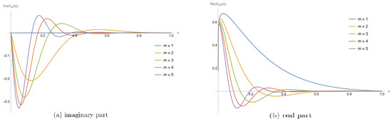
In our work to specify the eigenvalue of problem (10), using Wolfram Mathematica (high-level technical computing language) to calculate the values of ${\lambda }_m$ at different β, according to Lemma 2, we can rearrange all the zeros of $E_{\beta ,\beta }(-{\lambda }_m)$ as follows: $\dots {\lambda }_{-2},{\lambda }_{-1},{\lambda }_1,{\lambda }_2,\dots$. We observe, as shown in Table 1, that for $\beta ⟶1$, there is only a single real value and corresponding eigenfunction as shown in Figure 1, and with increasing β, we observe an increase in the number of real eigenvalues ${\lambda }_m$ with no complex when β is close to 2.

Table 1. The first five real and complex eigen values of Equation (10) at different $\beta$.

$\mathit{\beta }=$	$1.1$	$1.4$	$1.6$	$1.95$
${\lambda }_m$	$3.86752$	$4.68735$	$5.60788$	$9.00579$
	$10.7157\pm 7.36402I$	$16.2855$	$19.3929$	$35.6256$
	$14.8325\pm 15.3326I$	$25.8219$	$37.7632$	$78.8307$
	$18.8242\pm 23.3452I$	$44.8121\pm 10.6661I$	$61.3084$	$138.351$
	$23.0029\pm 31.3436I$	$68.9794\pm 25.9039I$	$200.772\pm 7.49232I$	$213.872$

Figure 1. The imaginary and real parts of egenfunctions ${\left\{P_m\left(\rho \right)\right\}}_{m=1}^5$ for Equation (10) at $\beta =1.1$.

The system ${\left\{P_m\left(\rho \right)\right\}}_{m=1}^{\infty }$ of eigenfunctions is complete but not orthogonal [19]. Thus, together with the system ${\left\{P_m\left(\rho \right)\right\}}_{n=1}^{\infty }$, we will consider the system ${\left\{{{\rm Y}}_m\left(\rho \right)\right\}}_{m=1}^{\infty }={\left\{{(1-\rho )}^{\beta -1}{E}_{\beta ,\beta }(-{\lambda }_m{(1-\rho )}^{\beta })\right\}}_{m=1}^{\infty }$, which represents the eigenfunctions of the adjoint of (10) and is biorthogonal with ${\left\{P_m\left(\rho \right)\right\}}_{m=1}^{\infty }$.

Equation (11) is solved in [20,21] by using the Laplace transform of the Caputo time fractional differential operator (2), where we obtain the solution in terms of the Mittage–Liffler function as $T_m={\varphi }_m{E}_{\alpha ,1}(-{\lambda }_m{t}^{\alpha })$, where the Fourier coefficient ${\varphi }_m$ is given by

$${\varphi }_m=\frac{⟨\varphi \left(\rho \right),{{\rm Y}}_m\left(\rho \right)⟩}{⟨P_m\left(\rho \right),{{\rm Y}}_m\left(\rho \right)⟩}.$$

(12)

Now, we can construct the solution of problem (8), where

$$z_1(\rho ,t)=\sum _{m=1}^{\infty }{T}_m\left(t\right)P_m\left(\rho \right)=\sum _{m=1}^{\infty }{\varphi }_m{E}_{\alpha ,1}(-{\lambda }_m{t}^{\alpha }){\rho }^{\beta -1}{E}_{\beta ,\beta }(-{\lambda }_m{\rho }^{\beta }).$$

(13)

By using Lemma (1) and the fact that for $T>0$,

$$|\frac{1}{E_{\alpha ,1}(-{\lambda }_m{T}^{\alpha })-1}|\le C_1,$$

(14)

$C_1$ is positive constant, where $E_{\alpha ,1}(-{\lambda }_m{T}^{\alpha })\ne 1$ [17]; it is not difficult to prove the solution of (13) is absolutely convergent.

Now we go to discuss the solution of Equation (9), $z_2(\rho ,t)$, which can be found by using the full basis of the eigenfunctions $P_m$

$$z_2(\rho ,t)=\sum _{m=1}^{\infty }{u}_m\left(t\right)P_m\left(\rho \right),s(\rho ,t)=\sum _{m=1}^{\infty }{s}_m\left(t\right)P_m\left(\rho \right),$$

(15)

where $s_m\left(t\right)=\frac{⟨s(\rho ,t),{{\rm Y}}_m\left(\rho \right)⟩}{⟨P_m\left(\rho \right),{{\rm Y}}_m\left(\rho \right)⟩}$. Then, from (9), we obtain

$$\begin{array}{cc}\hfill {}^C{D}_t^{\alpha }{u}_m\left(t\right)& +\left({\lambda }_m\right)u_m\left(t\right)=s_m\left(t\right),0<\alpha <1,\hfill \\ \hfill & u_m\left(0\right)=0.\hfill \end{array}$$

(16)

Applying the Laplace transform operator to both sides of Equation (16) [1], we have

$$u_m\left(t\right)={\int }_0^t{\tau }^{\alpha -1}{E}_{\alpha ,\alpha }(-{\lambda }_m{\tau }^{\alpha })s_m(t-\tau )d\tau ,$$

(17)

then, from (15), $z_2(\rho ,t)$ can formalize in the form

$$z_2(\rho ,t)=\sum _{m=1}^{\infty }\left({\int }_0^t{\tau }^{\alpha -1}{E}_{\alpha ,\alpha }(-{\lambda }_m{\tau }^{\alpha })s_m(t-\tau )d\tau \right){\rho }^{\beta -1}{E}_{\beta ,\beta }(-{\lambda }_m{\rho }^{\beta }),$$

(18)

Thus, from (7), (13) and (18), we obtain (6).

4. Numerical Solution of STFADE

In this section, the Crank—Nicholson finite difference technique is applied to obtain the numerical solution of one-dimensional STFADE (1) and present a numerical approximation for the Riemann–Liouville derivative. We find that if we assume for Equation(1) an equivalent partial integro-differential equation form, the precision of the discrete approximations could be improved. Let us try to take the fractional Riemman–Liouville integral $j_t^{\alpha },0<\alpha <1,$ on both sides of Equation (1) such that

$$j_t^{\alpha }f(\rho ,t)=\frac{1}{\Gamma \left(\alpha \right)}{\int }_0^t\frac{f(\rho ,\xi )}{{(t-\xi )}^{1-\alpha }}d\xi ,$$

(19)

Thus, we obtain

$$z(\rho ,t)=z(\rho ,0)+j_t^{\alpha }{(}_0^R{D}_{\rho }^{\beta }z(\rho ,t))+s(\rho ,t),$$

(20)

where $S(\rho ,t)=j_t^{\alpha }\left(s(\rho ,t)\right)$. In order to carry out discretizations, we introduced the temporal step size $\tau =\frac{T}{\aleph },\aleph \in \mathbb{Z}/\left\{0\right\}$ and uniform mesh of interval $[0,T],{\omega }_{\tau }=\{t_n: =n\tau ;0<n<\aleph \}$. Additionally, for a spatial discretization, let $\hslash =\frac{1}{\mathcal{M}},\mathcal{M}\in \mathbb{Z}/\left\{0\right\}$ and a uniform mesh of interval $[0,1],{\omega }_{\hslash }=\{{\rho }_i: =i\hslash ; 0<i<\mathcal{M}\}$. Suppose on ${\omega }_{\hslash }\times {\omega }_{\tau }$ there exists a grid function $\mathcal{W}=\left\{z_i^n|0\le i\le \mathcal{M},n\ge 0\right\},$ such that for any $z,v\in \mathcal{W},$ we define the following norms, semi-norm ${\parallel .\parallel }_{L^2}$ and the inner product [22], as follows:

$$\begin{array}{cc}\hfill z_i^{n+\frac{1}{2}}& =\frac{1}{2}\left[z_i^{n+1}+z_i^n\right],⟨z^n,g^n⟩=h{\displaystyle \sum _{i=1}^{\mathcal{M}-1}}{z}_i^n{g}_i^n,\hfill \\ \hfill \parallel z^n{\parallel }_{L^2}^2& =⟨z^n,z^n⟩\parallel z^n{\parallel }_{\infty }={\displaystyle \underset{0\le i\le \mathcal{M}}{max}}\left|z_i^n\right|,\hfill \\ \hfill ⟨{\delta }_{\rho }^{\beta }{z}^n,g^n⟩& =⟨{\delta }_{\rho }^{\beta /2}{z}^n,{\delta }_{\rho }^{\beta /2}{g}^n⟩.\hfill \end{array}$$

(21)

Additionally, we can represent the Riemann–Lioville fractional operator of any spatially dependent function $f\left(\rho \right)\in C^4\left(\mathbb{R}\right)$ by shifted the Grunwald–Letnikov formula as

$${}_0^R{D}_{\rho }^{\beta }f\left({\rho }_i\right)=\frac{1}{\Gamma (4-\beta ){\hslash }^{\beta }}\sum _{l=0}^{i+1}{q}_l^{\beta }f\left({\rho }_{i-l+1}\right)+O\left({\hslash }^2\right),$$

(22)

where

$$q_l^{\beta }=\left\{\begin{array}{cc}1,\hfill & l=0\hfill \\ 2^{3-\beta }-4,\hfill & l=1\hfill \\ 3^{3-\beta }-4.2^{3-\beta }+6,\hfill & l=2\hfill \\ {(l+1)}^{3-\beta }-4l^{3-\beta }+6{(l-1)}^{3-\beta }-4{(l-2)}^{3-\beta }+{(l-3)}^{3-\beta },\hfill & l\ge 3.\hfill \end{array}\right.$$

For time discretization, the high-order accuracy of the suggested method presented on the first-order approximation of the fractional Riemann–Liouville integral $j_t^{\alpha }$, this approximation established for every $f\left(t\right)\in C^{\alpha }\left([0,T]\right)$ that

$$j_t^{\alpha }f\left(t_n\right)={\tau }^{\alpha }\sum _{k=0}^n{p}_k^{\alpha }f\left(t_{n-k}\right)+O\left(\tau \right),$$

(23)

where $p_0^{\alpha }=1,p_k^{\alpha }={(-1)}^k\left(\genfrac{}{}{0pt}{}{-\alpha }{k}\right)$.

Lemma 3

([23]). The sequence ${\left\{q_l^{\beta }\right\}}_{l=0}^{\infty },1<\beta <2$, which is defined in (22), has the following properties

$$\sum _{l=0}^{\infty }{q}_l^{\beta }=0,q_1^{\beta }\le 0,q_0^{\beta }{\geqq }_3^{\beta }\ge \dots \ge 0,q_0^{\beta }+q_2^{\beta }\ge 0,q_2^{\left(\beta \right)}\left\{\begin{array}{cc}>0,\hfill & \beta \in ({\beta }_0,2)\hfill \\ \le 0,\hfill & \beta \in (1,{\beta }_0),\hfill \end{array}\right.$$

(24)

where ${\beta }_0$ is the zeros of $q_2^{\beta }$.

Lemma 4

([24]). The sequence ${\left\{p_k^{\alpha }\right\}}_{k=0}^{\infty },0<\alpha <1$, which is defined in (23), satisfies

$$p_k^{\alpha }>0,p_{k+1}^{\alpha }<p_k^{\alpha },p_{k+1}^{\alpha }+p_{k-1}^{\alpha }>2p_k^{\alpha },k\ge 1.$$

(25)

Lemma 5

([25]). Consider the sequence ${\left\{p_k^{\alpha }\right\}}_{k=0}^{\infty },0<\alpha <1$, which is defined in (22). Then, for any real vector ${({{\rm Y}}_1,{{\rm Y}}_2,\dots ,{{\rm Y}}_j,)}^T\in {\mathbb{R}}^j$, it holds that

$$\sum _{m=0}^{j-1}\left(\sum _{k=0}^m{p}_k^{\alpha }{{\rm Y}}_{m+1-k}\right){{\rm Y}}_{m+1}\ge 0$$

(26)

Therefore, according to discretization, ${\omega }_{\hslash }$ and ${\omega }_{\tau }$, a weighted Crank–Nicolson method for Equation (20) at the point $({\rho }_i,t_{n+\frac{1}{2}})$, produces

$$\begin{array}{cc}\hfill z({\rho }_i,t_{n+1})+& z({\rho }_i,t_n)=2z({\rho }_i,0)+{\tau }^{\alpha }({\displaystyle \sum _{k=0}^{n+1}}{p}_k^{\alpha }{\delta }_{\rho }^{\beta }z({\rho }_i,t_{n+1-k})\hfill \\ \hfill & +{\displaystyle \sum _{k=0}^n}{p}_k^{\alpha }{\delta }_{\rho }^{\beta }z({\rho }_i,t_{n-k}))+S({\rho }_i,t_{n+1})+S({\rho }_i,t_n)+R_i^{n+1},\hfill \end{array}$$

(27)

where $R_i^{n+1}<C(\tau +{\hslash }^2),C>0,0<i<\mathcal{M}-1,0<n<\aleph -1$.

Let $z_i^n$ represent the numerical solution of $z({\rho }_i,t_n),z_i^0=z({\rho }_i,0)$ and $S_i^n=S({\rho }_i,t_n)$. Tearranging the above Formula (27), we obtain the following weighted Crank–Nicolson numerical scheme for the one-dimensional STFADE (1):

$$\begin{array}{cc}\hfill z_i^{n+1}+& z_i^n=2z_i^0+{\tau }^{\alpha }\left({\displaystyle \sum _{k=0}^{n+1}}{p}_k^{\alpha }{\delta }_{\rho }^{\beta }{z}_i^{n+1-k}+{\displaystyle \sum _{k=0}^n}{p}_k^{\alpha }{\delta }_{\rho }^{\beta }{z}_i^{n-k}\right)\hfill \\ \hfill & +S_i^{n+1}+S_i^n,1<i<\mathcal{M}-1,1<n<\aleph -1,\hfill \\ \hfill z_0^n& =z_{\mathcal{M}}^n=0,0<n<\aleph ,\hfill \\ \hfill z_i^0& ={\varphi }_i,0<i<\mathcal{M}\hfill \end{array}$$

(28)

5. Analysis of the Numerical Solution

In this section, we will discuss the convergence and stability of the suggested numerical scheme (28).

Theorem 2.

Consider $z(\rho ,t)\in C^{\alpha ,2}\left(\omega \right),$ the solution of Equation (1), and consider that $\left\{Z_i^n\right|0\le i\le \mathcal{M},0\le n\le \aleph \}$ is the solution of the numerical scheme (28). Then, for small τ and ℏ, it holds that

$$\parallel {\Lambda }^n\parallel \le C(\tau +{\hslash }^2),$$

(29)

where ${\Lambda }_i^n=z({\rho }_i,t_n)-Z_i^n$.

Proof. 

Subtracting Equation (28) from Equation (27), we have

$$\begin{array}{cc}\hfill {\Lambda }_i^{n+1}+& {\Lambda }_i^n={\tau }^{\alpha }\left({\displaystyle \sum _{k=0}^{n+1}}{p}_k^{\alpha }{\delta }_{\rho }^{\beta }{\Lambda }_i^{n+1-k}+{\displaystyle \sum _{k=0}^n}{p}_k^{\alpha }{\delta }_{\rho }^{\beta }{\Lambda }_i^{n-k}\right)+R_{n+1}^i,\hfill \\ \hfill & {\Lambda }_i^0=0,0<i<\mathcal{M}-1,0<n<\aleph -1.\hfill \end{array}$$

(30)

Equation (30) can be rewritten in a matrix form as

$${\Lambda }^{n+1}+{\Lambda }^n=\sum _{k=0}^n{p}_k^{\alpha }A({\Lambda }^{n+1-k}+{\Lambda }^{n-k})+R_{n+1},$$

(31)

where

$${\Lambda }^n={({\Lambda }_1^n,{\Lambda }_2^n,\dots ,{\Lambda }_{\mathcal{M}-1}^n)}^T,A=\frac{{\tau }^{\alpha }}{\Gamma (4-\beta ){\hslash }^{\beta }}\left(\begin{array}{ccccc}{q}_1^{\left(\beta \right)}& q_0^{\left(\beta \right)}& 0& \cdots & 0\\ q_2^{\left(\beta \right)}& q_1^{\left(\beta \right)}& q_0^{\left(\beta \right)}& \cdots & \\ ⋮& q_2^{\left(\beta \right)}& q_1^{\left(\beta \right)}& \ddots & ⋮\\ ⋮& \cdots & \ddots & \ddots & q_0^{\left(\beta \right)}\\ q_{\aleph }^{\left(\beta \right)}& q_{\aleph -1}^{\left(\beta \right)}& \cdots & q_2^{\left(\beta \right)}& q_1^{\left(\beta \right)}\end{array}\right).$$

By the Gershgorin theorem and Lemma 3, we could investigate into the matrix A is negative definite matrix.

Multiplying Equation (31) by $\hslash {({\Lambda }^{n+1}-{\Lambda }^n)}^T$ in both sides, we obtain

$$\begin{array}{cc}\hfill \hslash {({\Lambda }^{n+1}-{\Lambda }^n)}^T({\Lambda }^{n+1}+{\Lambda }^n)& =\hslash {\displaystyle \sum _{k=0}^n}{p}_k^{\alpha }{({\Lambda }^{n+1}-{\Lambda }^n)}^{T}A({\Lambda }^{n+1-k}+{\Lambda }^{n-k})\hfill \\ \hfill & +\hslash {({\Lambda }^{n+1}-{\Lambda }^n)}^T{R}_{n+1}\hfill \end{array}$$

By using Lemma 5 and the fact that ${({\Lambda }^{n+1}-{\Lambda }^n)}^{T}A({\Lambda }^{n+1-k}+{\Lambda }^{n-k})<0$, we can deduce that

$$\parallel {\Lambda }^{n+1}{\parallel }^2-{\parallel {\Lambda }^n\parallel }^2\le ⟨R^{n+1},({\Lambda }^{n+1}-{\Lambda }^n)⟩,$$

By summing over n from 0 to $J-1$, it is deduced that

$$\parallel {\Lambda }^J{\parallel }^2\le \sum _{n=0}^{J-1}⟨R^{n+1},({\Lambda }^{n+1}-{\Lambda }^n)⟩\le ⟨R^J,{\Lambda }^J⟩\le C(\tau +{\hslash }^2)\parallel \Lambda \parallel .$$

(32)

Thus, we deduce (27). □

Theorem 3.

The numerical solution $\left\{Z_i^n\right|0\le i\le \mathcal{M},0\le n\le \aleph \}$ of scheme (28) is unconditionally stable and holds that

$$\parallel Z^J{\parallel }^2\le 2\parallel Z^0{\parallel }^2+\sum _{n=0}^{J-1}{\parallel (1+{\tau }^{\alpha }{p}_{n+1}^{\alpha }{\delta }_{\rho }^{\beta })Z^0+S^{n+\frac{1}{2}}\parallel }^2$$

(33)

Proof. 

Similar to the proof of Theorem 2, by multiplying Equation (28) by $\hslash (Z_i^{n+1}-Z_i^n)$ and obtaining the sum over i from $1⟶\mathcal{M}-1$,

$$\begin{array}{cc}\hfill \parallel Z^{n+1}{\parallel }^2-{\parallel Z^n\parallel }^2=& 2⟨Z^0,Z^{n+1}-Z^n⟩+{\tau }^{\alpha }{p}_{n+1}^{\alpha }⟨{\delta }_{\rho }^{\beta }{Z}^0,Z^{n+1}-Z^n⟩\hfill \\ \hfill & +{\tau }^{\alpha }{\displaystyle \sum _{k=0}^n}{p}_k^{\alpha }⟨{\delta }_{\rho }^{\beta }(Z^{n+1-k}+Z^{n-k}),Z^{n+1}-Z^n⟩\hfill \\ & +\frac{1}{2}⟨S^{n+\frac{1}{2}},Z^{n+1}-Z^n⟩.\hfill \end{array}$$

(34)

After applying the Cauchy=-Schwarz inequality and obtaining the sum of Equation (34) over n from 0 to $J-1$, we obtain

$$\begin{array}{cc}\hfill \parallel Z^J{\parallel }^2-{\parallel Z^0\parallel }^2=& 2{\displaystyle \sum _{n=0}^{J-1}}⟨Z^0,Z^{n+1}-Z^n⟩+{\tau }^{\alpha }{\displaystyle \sum _{n=0}^{J-1}}{p}_{n+1}^{\alpha }⟨{\delta }_{\rho }^{\beta }{Z}^0,Z^{n+1}-Z^n⟩\hfill \\ \hfill & +{\tau }^{\alpha }{\displaystyle \sum _{n=0}^{J-1}}{\displaystyle \sum _{k=0}^n}{p}_k^{\alpha }⟨{\delta }_{\rho }^{\beta }(Z^{n+1-k}+Z^{n-k}),Z^{n+1}-Z^n⟩\hfill \\ & +\frac{1}{2}{\displaystyle \sum _{n=0}^{J-1}}⟨S^{n+\frac{1}{2}},Z^{n+1}-Z^n⟩.\hfill \end{array}$$

(35)

Without loss of generality, according to Lemmas 4 and 5, we can infer that the second term on the right side of Equation (35) is negative, and by applying Young’s inequality, we obtain (33). □

6. Examples

In this section, we present an analytical and numerical solution of some examples for the one-dimensional STFADE (1). For particular values of $\alpha ,\beta ,s(\rho ,t),\varphi \left(\rho \right)$, we demonstrate the computational performance and theoretical findings of our suggested methods.

Example 1.

Consider

$$\begin{array}{cc}\hfill \frac{{\partial }^{\alpha }z(\rho ,t)}{\partial t^{\alpha }}& {=}_0^R{D}_{\rho }^{\beta }z(\rho ,t)+(\rho +{\rho }^{2-\beta })E_{\alpha ,1}(-t^{\alpha }),0<\alpha <1,1<\beta <2\hfill \\ \hfill z(0,t)& =z(1,t)=0,0<t<T,\hfill \\ \hfill z(\rho ,0)& =\rho (1-\rho ),0<\rho <1.\hfill \end{array}$$

(36)

Especially with (1), by setting $s(\rho ,t)=(\rho +{\rho }^{2-\beta })E_{\alpha ,1}(-t^{\alpha })$ and $\varphi \left(\rho \right)=\rho (1-\rho )$, we obtain (36), so the analytical solution of Equation (36) can be obtained using Theorem 1.

From the relation (4) and (5), one obtains

$$\begin{array}{cc}\hfill ⟨P_m\left(\rho \right),{{\rm Y}}_m\left(\rho \right)⟩& ={\int }_0^1{\rho }^{\beta -1}{E}_{\beta ,\beta }(-{\lambda }_m{\rho }^{\beta }){(1-\rho )}^{\beta -1}{E}_{\beta ,\beta }(-{\lambda }_m{(1-\rho )}^{\beta })d\rho \hfill \\ \hfill & =\frac{1}{\beta }{E}_{\beta ,2\beta -1}(-{\lambda }_m)-(\frac{1}{\beta }-1)E_{\beta ,2\beta }(-{\lambda }_m),\hfill \end{array}$$

(37)

$$\begin{array}{cc}\hfill ⟨\varphi \left(\rho \right),{{\rm Y}}_m\left(\rho \right)⟩& ={\int }_0^1(\rho -{\rho }^2){(1-\rho )}^{\beta -1}{E}_{\beta ,\beta }(-{\lambda }_m{(1-\rho )}^{\beta })d\rho \hfill \\ \hfill & =E_{\beta ,\beta +2}(-{\lambda }_m)-2E_{\beta ,\beta +3}(-{\lambda }_m),\hfill \end{array}$$

(38)

$$\begin{array}{cc}\hfill ⟨s(\rho ,t),{{\rm Y}}_m\left(\rho \right)⟩& =E_{\alpha ,1}(-t^{\alpha }){\int }_0^1(\rho +{\rho }^{2-\beta }){(1-\rho )}^{\beta -1}{E}_{\beta ,\beta }(-{\lambda }_m{(1-\rho )}^{\beta })d\rho \hfill \\ \hfill & =E_{\alpha ,1}(-t^{\alpha })(E_{\beta ,\beta +2}(-{\lambda }_m)+\Gamma (3-\beta )E_{\beta ,3}(-{\lambda }_m)),\hfill \end{array}$$

(39)

thus, from (12) and (15) can get ${\varphi }_m$ and $s_m\left(t\right)$, therefor,

$$\begin{array}{cc}\hfill {\int }_0^t& {\tau }^{\alpha -1}{E}_{\alpha ,\alpha }(-{\lambda }_m{\tau }^{\alpha })s_m(t-\tau )d\tau \hfill \\ \hfill & =\frac{\beta (E_{\beta ,\beta +2}(-{\lambda }_m)+\Gamma (3-\beta )E_{\beta ,3}(-{\lambda }_m))}{E_{\beta ,2\beta -1}(-{\lambda }_m)-(1-\beta )E_{\beta ,2\beta }(-{\lambda }_m)}{\int }_0^t{\tau }^{\alpha -1}{E}_{\alpha ,\alpha }(-{\lambda }_m{\tau }^{\alpha })E_{\alpha ,1}(-{(t-\tau )}^{\alpha })d\tau \hfill \\ \hfill & =\frac{\beta (E_{\beta ,\beta +2}(-{\lambda }_m)+\Gamma (3-\beta )E_{\beta ,3}(-{\lambda }_m))(E_{\alpha ,1}(-t^{\alpha })-E_{\alpha ,1}(-{\lambda }_m{t}^{\alpha }))}{(E_{\beta ,2\beta -1}(-{\lambda }_m)-(1-\beta )E_{\beta ,2\beta }(-{\lambda }_m))({\lambda }_m-1)}.\hfill \end{array}$$

(40)

Therefore,

$$z_1(\rho ,t)=\sum _{m=1}^{\infty }\frac{\beta (E_{\beta ,\beta +2}(-{\lambda }_m)-2E_{\beta ,\beta +3}(-{\lambda }_m))}{E_{\beta ,2\beta -1}(-{\lambda }_m)-(1-\beta )E_{\beta ,2\beta }(-{\lambda }_m)}{E}_{\alpha ,1}(-{\lambda }_m{t}^{\alpha }){\rho }^{\beta -1}{E}_{\beta ,\beta }(-{\lambda }_m{\rho }^{\beta })$$

(41)

and

$$z_2(\rho ,t)=\sum _{m=1}^{\infty }\frac{\beta (E_{\beta ,\beta +2}(-{\lambda }_m)+\Gamma (3-\beta )E_{\beta ,3}(-{\lambda }_m))(E_{\alpha ,1}(-t^{\alpha })-E_{\alpha ,1}(-{\lambda }_m{t}^{\alpha }))}{(E_{\beta ,2\beta -1}(-{\lambda }_m)-(1-\beta )E_{\beta ,2\beta }(-{\lambda }_m))({\lambda }_m-1)}{\rho }^{\beta -1}{E}_{\beta ,\beta }(-{\lambda }_m{\rho }^{\beta })$$

(42)

from (7), we get the analytical solution $z(\rho ,t)$ of (36).

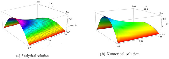
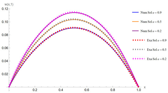
The compression of the proposed numerical scheme (28) for solving (36) with the numerical solution $Z_i^n$ and its analytical solution $z(\rho ,t)$ for $\beta =1.9$ and different α values is shown in Figure 2 at $t=T=1$. Figure 3 shows the graphical analytical and numerical solution of (36). The error is analyzed as the following $L_2$-norm

$$\Lambda (\tau ,\hslash )=\sqrt{\hslash {\displaystyle \sum _{i=1}^{\mathcal{M}-1}}{|z({\rho }_i,t_{\aleph })-Z_i^{\aleph }|}^2},$$

(43)

and the order of the convergence can be calculated as

$$R_t\simeq {log}_2\left[\frac{\Lambda (\tau ,\hslash )}{\Lambda (2\tau ,\hslash )}\right],$$

(44)

Figure 2. The analytical and numerical solution of (36) for $\alpha =0.5,\beta =1.9$ and $T=1$.

Figure 3. The analytical and numerical solution of (36) for different $\alpha =0.2,0.5,0.9,\beta =1.9$ and $t=T=1$.

Furthermore, in Table 2, we fix the space step at $\hslash =0.02,T=1$, and analyse how the error of the proposed numerical scheme for solving (36) ($\Lambda (\tau ,\hslash )$) changes with the maximum less than $O(\tau ,{\hslash }^2)$.

Table 2. The error and convergence rate when $\hslash =0.02$ and $\beta =1.9,T=1$.

	$\mathit{\alpha }=0.2$		$\mathit{\alpha }=0.5$		$\mathit{\alpha }=0.7$		$\mathit{\alpha }=0.9$
$\tau$	$\Lambda (\tau ,\hslash )$	$R_t$	$\Lambda (\tau ,\hslash )$	$R_t$	$\Lambda (\tau ,\hslash )$	$R_t$	$\Lambda (\tau ,\hslash )$	$R_t$
1/20	$5.8547\times {10}^{-4}$		$5.2961\times {10}^{-4}$		$4.9107\times {10}^{-4}$		$4.4985\times {10}^{-4}$
1/40	$2.9077\times {10}^{-4}$	$1.0097$	$2.5737\times {10}^{-4}$	$1.0410$	$2.4105\times {10}^{-4}$	$1.0265$	$2.1869\times {10}^{-4}$	$1.04053$
1/80	$1.5035\times {10}^{-4}$	$0.9515$	$1.3682\times {10}^{-4}$	$0.9115$	$1.1948\times {10}^{-4}$	$1.0125$	$1.0524\times {10}^{-4}$	$1.0552$
1/160	$7.9782\times {10}^{-5}$	$0.9142$	$6.6193\times {10}^{-5}$	$1.0475$	$5.8716\times {10}^{-5}$	$1.0250$	$4.9792\times {10}^{-5}$	$1.0797$
1/320	$3.8468\times {10}^{-5}$	$1.0526$	$3.1851\times {10}^{-5}$	$1.0553$	$2.9153\times {10}^{-5}$	$1.0101$	$2.4790\times {10}^{-5}$	$1.0060$

7. Conclusions

In this paper, we intend to consider the general form of STFADE with time and fractional derivatives defined in the Caputo and Riemann–Liouville sense by fractional order derivatives $0<\alpha <1 and 1<\beta <2$, respectively. The analytical solution of one dimension STFADE is carried out by Fourier methods. The justification of the basis for the system of eigenfunctions and their corresponding eigenvalues for the basic Equation (10) is based on the asymptotic properties of zeros of the two-parameter Mittag–Leffler function. The Crank–Nicolson finite difference technique is applied to construct the unconditional stable proposed scheme of the equivalent partial integro-differential Equation (20). The proposed numerical scheme is convergent with first-order accuracy in the temporal direction and second-order accuracy in the spatial direction. All the numerical experiments support our theoretical results. Model (1) may be considered in future work with different definitions of fractional derivatives and different methods for numerical and analytical solutions.

References

- Podlubny, I. Fractional Differential Equations; Academic Press: New York, NY, USA, 1999. [Google Scholar]
- Sabatier, J.; Agrawal, O.P.; Machado, A.T. Advances in Fractional Calculus. In Theoretical Developments and Applications in Physics and Engineering; Springer: Dordrecht, The Netherlands, 2007. [Google Scholar]
- Aleroev, M.; Aleroev, H.; Aleroev, T. Proof of the completeness of the system of eigenfunctions for one boundary-value problem for the fractional differential equation. AIMS Math. 2019, 4, 714–720. [Google Scholar] [CrossRef]
- Gorenflo, R.; Mainardi, F. Random Walk Models for Space Fractional Diffusion Processes. Fract. Calc. Appl. Anal. 1998, 1, 167–191. [Google Scholar]
- Mainardi, F.; Luchko, Y.; Pagnini, G. The fundanental solution of the space-time fractional diffusion equation. Fract. Calc. Appl. Anal. 2001, 4, 153–192. [Google Scholar]
- Shymanskyi, V.; Sokolovskyy, Y. Variational Method for Solving the Viscoelastic Deformation Problem in Biomaterials with Fractal Structure. In Proceedings of the Information Technology and Implementation (IT&I-2021), CEUR Workshop Proceedings, online, 1–3 December 2021; pp. 125–134. [Google Scholar]
- Shymanskyi, V.; Sokolovskyy, Y.; Boretska, I.; Sokolovskyy, I.; Markelov, O.; Storozhuk, O.M. Application of FEM with Piecewise Mittag-Leffler Functions Basis for the Linear Elasticity Problem in Materials with Fractal Structure. In Proceedings of the 2021 IEEE XVIIth International Conference on the Perspective Technologies and Methods in MEMS Design (MEMSTECH), Lviv, Ukraine, 12–16 May 2021; pp. 16–19. [Google Scholar]
- Alidousti, J.; Ghafari, E. Dynamic behavior of a fractional order prey-predator model with group defense. Chaos Solitons Fractals 2020, 134, 109688. [Google Scholar] [CrossRef]
- Rihan, F.A.; Rajivganthi, C. Dynamics of fractional-order delay differential model of prey-predator system with Holling-type III and infection among predators. Chaos Solitons Fractals 2020, 141, 110365. [Google Scholar] [CrossRef]
- Alidousti, J.; Ghahfarokhi, M.M. Stability and bifurcation for time delay fractional predator prey system by incorporating the dispersal of prey. Appl. Math. Model. 2019, 72, 385–402. [Google Scholar] [CrossRef]
- Xu, C.; Zhang, W.; Aouiti, C.; Liu, Z.; Yao, L. Further analysis on dynamical properties of fractional-order bi-directional associative memory neural networks involving double delays. Math. Methods Appl. Sci. 2022, 1–19. [Google Scholar]
- Alidousti, J. Stability and bifurcation analysis for a fractional prey–predator scavenger model. Appl. Math. Model. 2020, 81, 342–355. [Google Scholar] [CrossRef]
- Aleroev, T. Solving the Boundary Value Problems for Differential Equations with Fractional Derivatives by the Method of Separation of Variables. Mathematics 2020, 8, 1877. [Google Scholar] [CrossRef]
- Mahmoud, E.; Orlov, V.N. Numerical Solution of Two Dimensional Time-Space Fractional Fokker Planck Equation with Variable Coefficients. Mathematics 2021, 9, 1260. [Google Scholar] [CrossRef]
- Sandev, T.; Zivorad, T. The general time fractional wave equation for a vibrating string. J. Phys. A Math. Theor. 2010, 43, 055204. [Google Scholar] [CrossRef]
- Aleroev, T.S.; Elsayed, A.M. Analytical and Approximate Solution for Solving the Vibration String Equation with a Fractional Derivative. Mathematics 2020, 8, 1154. [Google Scholar] [CrossRef]
- Gorenflo, R.; Kilbas, A.A.; Mainardi, F.; Rogosin, S.V. Mittag-Leffler Functions Related Topics and Applications; Springer: New York, NY, USA, 2014. [Google Scholar]
- Aleroev, T.S.; Elsayed, A.M.; Mahmoud, E.I. Solving one dimensional time-space fractional vibration string equation. IOP Mater. Sci. Eng. Conf. Ser. 2021, 1129, 012030. [Google Scholar] [CrossRef]
- Aleroev, T.S.; Kirane, M.; Tang, Y. The boundary-value problem for a differential operator of fractional order. J. Math. Sci. 2013, 194, 499–512. [Google Scholar] [CrossRef]
- Ali, M.; Aziz, S.; Malik, S. Inverse source problems for a space-time fractional differential equation. Inverse Probl. Sci. Eng. 2020, 28, 47–68. [Google Scholar] [CrossRef]
- Al-Refai, M.; Luchko, Y. Maximum Principle for the Multi-Term Time-Fractional Diffusion Equations with the Riemann-Liouville Fractional Derivatives. Appl. Math. Comput. 2015, 257, 40–51. [Google Scholar] [CrossRef]
- Wang, P.D.; Huang, C.M. An energy conservative difference scheme for the nonlinear fractional Schrödinger equations. J. Comput. Phys. 2015, 293, 238–251. [Google Scholar] [CrossRef]
- Sousa, E.; Li, C. A weighted finite difference method for the fractional diffusion equation based on the riemann–liouville derivative. Appl. Numer. Math. 2015, 90, 22–379. [Google Scholar] [CrossRef]
- Lubich, C. Discretized fractional calculus. SIAM J. Math. Anal. 1986, 17, 704–719. [Google Scholar] [CrossRef]
- Tang, T. A finite difference scheme for partial integro-differential equations with a weakly singular kernel. Appl. Numer. Math. 1993, 11, 309–319. [Google Scholar] [CrossRef]
Publisher’s Note: MDPI stays neutral with regard to jurisdictional claims in published maps and institutional affiliations. |
© 2022 by the authors. Licensee MDPI, Basel, Switzerland. This article is an open access article distributed under the terms and conditions of the Creative Commons Attribution (CC BY) license (https://creativecommons.org/licenses/by/4.0/).