Article

MSDA-NMF: A Multilayer Complex System Model Integrating Deep Autoencoder and NMF

1
College of International Business, Zhejiang Yuexiu University, Shaoxing 312000, China
2
Shaoxing Key Laboratory of Intelligent Monitoring and Prevention of Smart Society, Shaoxing 312000, China
3
Tianjin Key Laboratory of Advanced Networking (TANK), College of Intelligence and Computing, Tianjin University, Tianjin 300350, China
4
Graduate Business School, UCSI University, Kuala Lumpur 56000, Malaysia
*
Authors to whom correspondence should be addressed.
Mathematics 2022, 10(15), 2750; https://doi.org/10.3390/math10152750
Submission received: 30 June 2022 / Revised: 26 July 2022 / Accepted: 1 August 2022 / Published: 3 August 2022

Abstract

:
In essence, the network is a way of encoding the information of the underlying social management system. Ubiquitous social management systems rarely exist alone and have dynamic complexity. For complex social management systems, it is difficult to extract and represent multi-angle features of data only by using non-negative matrix factorization. Existing deep NMF models integrating multi-layer information struggle to explain the results obtained after mid-layer NMF. In this paper, NMF is introduced into the multi-layer NMF structure, and the feature representation of the input data is realized by using the complex hierarchical structure. By adding regularization constraints for each layer, the essential features of the data are obtained by characterizing the feature transformation layer-by-layer. Furthermore, the deep autoencoder and NMF are fused to construct the multi-layer NMF model MSDA-NMF that integrates the deep autoencoder. Through multiple data sets such as HEP-TH, OAG and HEP-TH, Pol blog, Orkut and Livejournal, compared with 8 popular NMF models, the Micro index of the better model increased by 1.83 , NMI value increased by 12 % , and link prediction performance improved by 13 % . Furthermore, the robustness of the proposed model is verified.

1. Introduction

Non-negative matrix factorization (NMF) is now known to be a relatively new method of matrix factorization [1]. Since D.D. Lee et al. proposed a new method of feature subspace in Nature in 1999, Non-negative Matrix Factorization [2] has been widely used in image analysis, text clustering, data mining, speech processing and other aspects. With the deepening of research, many application analyses have developed, from the early single-structure feature analysis to the joint mining of multiple network structures and the layered analysis of multi-source information. In addition, abundant data indicate that the model based on a single pairwise interaction may not capture complex dependencies between network nodes [3]. The interaction of user with both the video and its enrichments results in a lot of explicit and implicit relevance feedback, which enables some works to provide personalized and rich multimedia content [4]. Lambiotte and Rosvall et al. [5] described the shortcomings of the traditional network model and the existing ideal high-order model in their article published in NaturePhysics and discussed that the multi-layer network model played an important role in the analysis of various types of interactions of many actual complex systems.
In the analysis and mining of multi-relational data, the method based on network representation learning has attracted the attention of many scholars because of its excellent performance in many practical tasks. Network representation learning [6] (also known as network embedding) is an effective network analysis method. Based on preserving network structure information, it embeds graphs into a low-dimensional and compact space. For complex multi-level data, however, with only the NMF decomposition single-layer network composed of a single decomposition, it tends to reach a higher accuracy even with the corruption of a severe proportion of data, as well as the function of the local minimum in split, leaving it unable to express the characteristics of data from many angles, so decomposition results are not always satisfied [7].
To effectively represent high-order and multi-layer complex data, traditional vector-based machine learning and deep learning algorithms can directly use the mapping of low-dimensional space representations to efficiently complete network analysis tasks, which greatly enrich the selection of algorithms and models for network mining tasks [8,9]. Therefore, how to use an effective deep network structure for the hierarchical feature extraction of complex data and how to combine the advantages of non-negative matrix decomposition and deep networks have important practical implications for the collaborative discovery of data research knowledge from multiple information sources.
Therefore, in this paper, NMF is introduced into a multi-layer NMF structure, and the feature representation of input data is realized by using a complex hierarchical structure. By adding regularization constraints for each layer, the essential features of data are obtained by characterizing the feature transformation layer-by-layer, and further, the multi-layer NMF model MDA-NMF of a deep autoencoder and NMF is constructed. The method proposed in this paper can effectively improve the detection accuracy and prediction accuracy of social groups in the complex social management system. The main contributions of the proposed system can be summarized as follows: 1. The model integrates the multi-layer structure features of deep self-coding; 2. The model introduces multi-layer NMF structure, which can effectively use a complex hierarchical structure to achieve feature representation of input data; 3. Through the evaluation of multiple data sets, it is proved that the proposed method is superior to the existing multi-layer NMF method.
The rest of the paper is organized as follows: Section 2 discusses the related work. Section 3 introduces the proposed method through model description and model optimization. The experimental results are shown in Section 4 and discussed by parametric sensitivity analysis, multiclassification experiment, node clustering experiment, and link prediction experiment. Finally, Section 5 introduces the conclusion.

2. Materials and Methods

2.1. Study on Non-Negative Matrix Factorization

Non-negative matrix factorization is a popular machine learning technique. The essence of a non-negative matrix algorithm is to transform high-dimensional data into low-dimensional data by a linear combination of variables. There is non-negative value in the decomposition result, which dramatically improves the interpretability of the model, and development is also a widespread concern. In 2001, Lee and Seung put forward the multiplicative iteration algorithm [10], and from then the NMF algorithm was widely used in areas such as NLP, CV, a recommendation system and other fields. However, as the result of matrix decomposition, the feature matrix and coefficient matrix are not sparse enough, so the feature extraction is not apparent enough. Therefore, researchers have begun to study the sparsity of the feature matrix and coefficient matrix, and the repeatability of data in the feature matrix and sparse matrix will also be reduced. Similarly, many methods have been proposed. For example, Hoyer et al. [11] reconstructed the data and established the objective function by calculating the error between the actual and Euclidean distances. In addition, L1 was added as the penalty term, and the eigenmatrix and coefficient moment were optimized by iteration through the gradient descent method. Ren et al. [12] first used the given reference image to create nonorthogonal and non-negative basis components and then used these components to model the target. A factor then scales the constructed model to compensate for the contribution from the disk. Jia et al. [13] proposed a new semi-supervised model that simultaneously learns similar matrices with supervised information and generates clustering results. Huang et al. [14] proposed a robust multi-feature collective non-negative matrix decomposition (RMCNMF) model for ECG biometric noise and sample variation.
In summary, many studies implement complex function approximation and learn data sets from small sample sets through distributed representation of input data. Therefore, more and more researchers have focused on deep non-negative matrix factorization based on deep learning.

2.2. Deep Non-Negative Matrix Decomposition Analysis

The development of deep learning has gone through a long process. SVM, Boosting, Logistic Regression (LR) and other methods have been successively proposed. The structures of these methods either have no hidden layer nodes or contain a layer of them, so they are collectively referred to as shallow layer models. In 2006, The DBN (Deep Belief Network) model proposed by Hinton et al. [15] made it possible to construct Deep models for learning. Subsequently, deep models such as Deep Boltzmann Machines (DBM) [16] and Fuzzy Deep Belief Networks (FDBN) [17] were successively proposed. These deep networks with multiple hidden layers have excellent feature learning abilities. The features acquired by learning have an essential description of data, which is more favourable in visualization or classification applications. Ye et al. [18] proposed a new model for community detection—Depth-like autoencoder NMF (DANMF) based on the deep non-negative matrix method. DANMF adopts the architecture of hierarchical mapping between the original network and the final network community allocation and implicitly learns the hidden attributes from the low-level to the high-level of the original network in the middle layer. According to the deep decomposition architecture, De et al. [19] reviews the MF model based on deep learning and introduces the algorithm and application.
Because of deep networks’ excellent data learning performance, some scholars have proposed multi-layer non-negative matrix decomposition algorithms based on NMF and related algorithms in recent years [20]. However, the above methods and the deep NMF model integrating multi-layer information struggle to explain the results of the middle layer NMF.

2.3. Multilayer Non-Negative Matrix Factorization

Unlike single-layer learning, multi-layer NMF reveals more intuitive feature levels through the relationship between features of each layer. Layered structures learn meaningful and helpful features. The first model to extend CLRMA to multiple levels was the multi-layer NMF proposed by Cichocki et al., 2006 [21,22]. At the first level, the low-rank factor factorization of X is computed. At the next level, the matrix factorization is performed until the matrix factorization is performed. In 2013, a hierarchical non-negative matrix decomposition algorithm was proposed by [23] for hierarchical data representation. Multi-layer NMF obtains a multi-layer structure through multiple iterations of a nonsmooth non-negative matrix decomposition algorithm. Rajabi et al. [24] proposed using multi-layer NMF (MLNMF) to achieve hyperspectral decomposition. The spectral eigenmatrices are modelled as the product of sparse matrices. Chen et al. [25] proposed a constrained multi-layer NMF method for hyperspectral data processing. In this approach, at each level, and two constraints are implemented on the objective function. One is the sparsity on the abundance matrix, and the other is the minimum volume on the spectral matrix. The hierarchical processing decomposed the abundance matrix into a series of matrices, making the sparsity feature more evident and meaningful. Yuan et al. [26] introduced Hoyer projectors to provide the iterative directivity of structures in the decomposition of processes. They proposed a multi-layer non-negative matrix decomposition framework based on Hoyer projection—HP-MLNMF, which completely reconstructed and enhanced the methods.
However, in the above methods, there are few studies on the description of the middle layer of multi-layer network and the fusion model of NMF.

2.4. Encoder-Based Model

The basic idea is to map the context matrix to the embedding matrix and then use the embedding matrix to reconstruct the original context matrix. Deep neural graph representation (DNGR) [27], Structural Deep Network Embedding (SDNE) [28] and MVC-DNE [29] use deep neural networks to combine graph structures into coder algorithms directly. The basic idea behind these methods is to use autoencoders to compress information approximately node-local neighbor characteristics. The key to SDNE’s ability to preserve node neighbour characteristics is deep autoencoders and multiple nonlinear layers. The model is used to protect first and second-order approximations of nodes by using Laplacian features in the middle layers of the encoder and by using modified autoencoder reconstruction errors. In addition to the domain autoencoder method mentioned above, there is also an encoder method that iteratively aggregates domain information to generate node embedding [30] and the GraphSAGE algorithm [31]. Researchers design encoders that rely on node-local neighbor characteristics rather than the whole graph and use node embedding methods to overcome significant limitations of shallow embedding and self-coding methods.
To sum up, most of the research based on the encoder model are based on local graphs, and few on multi-layer global graphs.

3. Proposed Model

3.1. Model Description

There is only one layer of mapping between the original network and the embedded result features. The organization patterns of real-world networks is complex and diverse, and the mapping of the original network and community member space is likely to contain not only complex hierarchical and structural information, but also imply low-level hidden features, which cannot be extracted using classical shallow NMF-based methods. Furthermore, deep autoencoders are an excellent scheme for bridging the gap between low-level and high-level abstractions of raw data [32]. Inspired by the deep autoencoders, we can assume that we can obtain better structural features between nodes (i.e., more accurate structural feature matrix V) by further decomposition of mapping V and quality extraction at a deeper level from a lower to a higher level.
Based on the above discussion, this paper proposes a new model called the fusion deep autoencoder multi-layer STRUCTURE NMF model (MSDA-NMF). NMF introduces a multi-layer NMF structure and combines a deep autoencoder with NMF. Figure 1 illustrates an encoder component and a decoder component constituting the MSDA-NMF with a deep structure. Similar to the deep autoencoder, the encoder component attempts to transform raw networks into a low-dimensional hidden feature matrix captured in the middle layer. Like the deep autoencoder, the encoder component changes the primary network into a low-dimensional invisible feature matrix captured in the middle layer. Every intermediate layer explains the resemblance between nodes of various sequence. The decoder has symmetry with the encoder. It reconstructs the original network from the final embedded eigenmatrix through the hierarchical mapping learned in the encoder component. Unlike traditional NMF-based loss functions that only consider the decoder components, MSDA-NMF integrates encoder components and decoder components into unified loss functions.Using this method, the quasi-autoencoder NMF can learn the relationships between cross-layer features and obtain the extraction process from first-order to the high-order similarity of network structure in complex data intuitively and easily. MSDA-NMF using this hierarchical structure feature extraction algorithm, the optimal depth class autoencoder class NMF structure suitable for classification tasks is studied.
To better explain the terms and symbols used in this paper, we have unified the terms and symbols used. See Table 1 for details.

3.1.1. Model Solution

NMF directly learns a layer of auxiliary matrix Z and basis matrix V . However, real-world networks are often complex and diverse organizational patterns. Therefore, the mapping between the original network and the community member space will probably contain complicated hierarchical and structural information with implicit low-level hidden attributes. It is well known that deep learning can bridge the gap between low-level and high-level abstractions of raw data. In this sense, we propose to factor the mapping Z further, hoping to add an extra layer of abstraction for each layer of embedding results and extract the similarity between nodes from low order to high order. To be specific, the adjacency matrix A is decomposed into the product of p + 1 non-negative matrices, as follows:
A Z 1 Z 2 Z p V p
Thereinto V p R k × n , Z i R r i 1 × r i ( 1 i 3 ) , request n = n 0 r 1 r p 1 r p = k .
A hierarchy in Formula (1) that allows p-level abstract understanding of the original network can look similar to the following Sample decomposition:
V p 1 Z p V p , V 2 Z 3 V 3 , V 1 Z 2 Z 3 V 3 .
We also retain the non-negative constraint V i ( 1 i p ) . V i is the embedded characteristic matrix of the i layer, and Z i is the auxiliary matrix of the i layer. By doing so, each layer of abstract V i captures node similarity of different orders, from first-order proximity to structural identification and finally to community-level similarity. To learn the embedding matrix, we derive the following objective function. This paper uses a three-layer NMF structure, so p = 3 :
m i n Z i , V p L D = A Z 1 Z 2 Z 3 V 3 F 2 s . t . , Z i 0 , V p 0 , i = 1 , 2 , , p .
After the optimization of Formula (3), we can obtain the learning result of a network representation of each layer V i ( i < p ) by A Z 1 Z 2 Z 3 V 3 F 2 as [33].

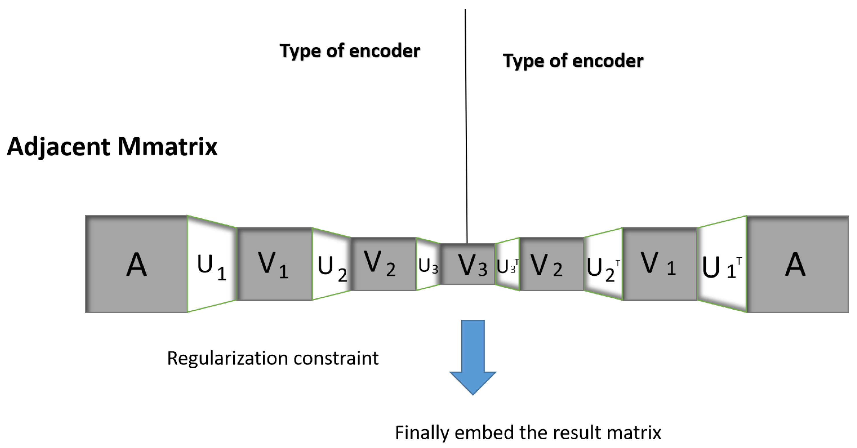
3.1.2. Fusion Depth-like Autoencoder Matrix Decomposition

It can be seen that Formula (1) is a reconstruction of the original network corresponding to the decoder part of the autoencoder. To improve the representation learning capability of the auto encoder, the encoder components must be integrated into the community detection model based on NMF to form the NMF model similar to the autoencoder. The rationality of the NMF model of class automatic coders is quite simple. For the ideal basis matrix V , it is supposed to be able to reconstruct the primal network by reconstructing the mapping Z with a small error; meanwhile, it should be able to precisely project the primal network Z to the community membership space by the help of the mapping Z , that is, V = Z T A . Integrating the encoder component and the decoder component with a unified loss function allows them to know each other during the learning process, from which we can obtain the ideal community members of the node. To accomplish this vision in the depth model, the objective function of the encoder is as follows.
m i n Z i , V p L E = V 3 Z 3 T Z 2 T Z 1 T A F 2 s . t . , Z i 0 , V p 0 , i = 1 , 2 , , p .
The current deep class autoencoder matrix decomposition model cannot explain what kind of network representation results can be obtained at the impenetrable levels. To enhance the interpretability of this model, we add standard terms for different levels. In [34], the second-order similarity matrix of LINE is expressed in the form:
C = l o g ( v o l ( G ) D 1 AD 1 ) l o g b ,
l o g ( . ) is the logarithm of all the matrix elements, D is the degree matrix of graph G, D = d i a g ( d 1 , d 2 , , d | V | ) , and b is the negative sampling parameter. v o l ( G ) is the capacity of the graph. G , v o l ( G ) = i j A i j .
The final objective function is:
m i n Z i , V p L = L D + L E + α Z 1 T Z 2 Z 3 V 3 F 2 + β Z 3 V 3 C + γ WV 3 B s . t . , Z i 0 , V p 0 , i = 1 , 2 , , p .
In this way, the first-order similarity of the network structure can be obtained after first-layer non-negative matrix decompositions, the second-order similarity of the network structure can be obtained after second-layer non-negative matrix decompositions, and higher-order features can be obtained after third-layer non-negative matrix decompositions.

3.2. Model Optimization

Optimization problems are highly related to scientific research [35], and in this paper in order to speed up the model’s approximation of the factor matrix, we pretrain each layer to obtain the initial approximation Z i and V i of the factor matrix. The training time of the model can be significantly reduced by the pretraining process. The effectiveness of pretraining has been proven in deep autoencoder networks. For pretraining, we first decompose the adjacency matrix A Z 1 V 1 by minimizing A Z 1 V 1 F 2 + V 1 Z 1 T A F 2 . Then, we decompose the matrix V 1 into V 1 Z 2 V 2 by minimizing V 1 Z 2 V 2 F 2 + V 2 Z a T A F 2 . The third layer is similar. Then, fine-tuning the objective function (6) for each layer by alternately minimizing the objective function proposed in the equation until the update of the objective function is very small, that is, the convergence ends. The updated algorithm is shown in the objective function of Algorithm 1.
Algorithm 1: Optimization of MSDA-NMF model
Mathematics 10 02750 i001
The objective function (6) requires a parameter matrix consisting of V 3 , Z 1 , Z 2 , Z 3 , W , and their update rules are introduced in detail below. So here we have U = Z 1 Z 2 Z 3 .

3.2.1. V 3 Subproblems

When V 3 is updated, the matrices Z 1 , Z 2 , Z 3 and W are fixed to obtain the objective function is Equation (6).
By introducing Lagrangian multiplication matrix Θ , the following can be obtained:
L ( V 3 ) = t r ( AA T AV 3 T U T U V 3 A T + U V 3 T U ) T + t r ( V 3 V 3 T V 3 A T ( U ) Z 3 T Z 2 T Z 1 T AV 3 T + Z 3 T Z 2 T Z 1 T AA T U ) + α t r ( Z 1 Z 1 T Z 1 V 3 Z 3 T Z 2 T Z 2 Z 3 V 3 Z 1 + Z 2 Z 3 V 3 V 3 T Z 3 T Z 2 T ) + β t r ( Z 3 V 3 V 3 T Z 3 T Z 3 V 3 B T BV 3 T Z 3 T + BB T ) + γ t r ( WV 3 V 3 T W T WV 3 C T C V 3 C T CV 3 T W T + CC T ) + t e ( Θ V 3 )
Let α L ( V 3 ) α V 3 = 0 be obtained:
A T U U T A + 2 V 3 U T U + 2 V 3 2 U T A + α ( 2 Z 2 Z 3 T Z 1 T Z 2 Z 3 T Z 1 T + 2 Z 2 Z 3 T Z 2 Z 3 ) + β ( Z 3 T Z 3 Z 3 T B Z 3 T B ) + γ ( 2 W T W 2 W T C ) + Θ = 0
Initialize V 3 and update V 3 according to the following rules:
V 3 V 3 2 U T A + 2 α Z 2 Z 3 T Z 1 T + 2 β Z 3 T B + 2 γ W T C A T U + 2 V 3 U T U + 2 V 3 + 2 α Z 2 Z 3 T Z 2 Z 3 + β Z 3 T Z 3 + 2 γ W T WV 3

3.2.2. Z 1 Subproblem

When updating Z 1 , other variables are fixed to receive the following objective function:
A U V 3 F 2 + V 3 Z 3 T Z 2 T Z 1 T A F 2 + α Z 1 T Z 2 Z 3 V 3 F 2
Similar to the update matrix V 3 , Lagrangian multiplication matrix Θ is introduced to obtain:
L ( Z 1 ) = t r ( AA T A U T Z 1 T ) U V 3 A T + U V 3 V 3 T Z 3 T Z 2 T Z 1 T + t r ( V 3 V 3 T V 3 A T U Z 3 T Z 2 T Z 1 T AV 3 T + Z 3 T Z 2 T Z 1 T AA T U ) + α t r ( Z 1 T Z 1 Z 1 ( Z 2 Z 3 V 3 ) T Z 2 Z 3 V 3 Z 1 + Z 2 Z 3 V 3 ( Z 2 Z 3 V 3 ) T ) + t r ( Θ Z 1 )
Identical to the optimization calculation of V 3 , we define the update rules of Z 1 as follows:
Z 1 Z 1 A ( Z 2 Z 3 V 3 ) T + AV 3 T Z 3 T Z 2 T + α ( Z 2 Z 3 V 3 ) T U V 3 V 3 T Z 3 T Z 2 + AA T U ( Z 2 Z 3 ) T + α Z 1

3.2.3. Z 2 Subproblem

When Z 2 is updated, other variables are fixed and the following objective function is obtained:
A U V 3 F 2 + V 3 Z 3 T Z 2 T Z 1 T A F 2 + α Z 1 T Z 2 Z 3 V 3 F 2
Referring to the V 3 optimization algorithm, we define the update rules of Z 2 as follows:
Z 2 Z 2 2 Z 1 T AV 3 T Z 3 T + α Z 1 T V 3 T Z 3 T Z 1 T U V 3 V 3 T Z 3 T + Z 1 T AA T U T Z 3 + α Z 2 Z 3 V 3 V 3 T Z 3

3.2.4. Z 3 Subproblem

When updating Z 3 , fix other variables and obtain the following objective function:
m i n Z i , V p L = L D + L E + α Z 1 T Z 2 Z 3 V 3 F 2 + β Z 3 V 3 C
Refer to the V 3 optimization algorithm, we define the update rules of Z 3 as follows:
Z 3 Z 3 2 U 2 T U 1 T A V 3 T + 2 U 2 T U 1 T A V 3 T + 2 α Z 2 T Z 1 T V 3 + β ( BV 3 T Z 3 T + BV 3 T ) 2 Z 2 T Z 1 T U V 3 V 3 T + 2 Z 2 T Z 1 T AA T U + 2 α Z 2 T Z 2 Z 3 V 3 V 3 T + β Z 3 V 3 V 3 T

3.2.5. W Subproblem

When W is updated, other variables are fixed and the following objective function is obtained:
γ WV 3 C F 2
Refer to the V 3 optimization algorithm, we define the update rule of W as follows:
W W C W V 3

3.2.6. Model Complexity Analysis

The computational complexity of the five updated formulas in algorithm Algorithm 1 is respectively O ( r 1 r 2 r 3 n 2 + r 1 r 2 r 3 n + r 2 r 3 n + r 1 2 r 2 2 r 3 2 n + r 2 2 r 3 n ) , O ( r 3 n 2 + r 2 r 3 n + r 1 r 2 n + n 3 + r 1 n 2 ) , O ( r 1 n 2 + r 1 r 3 n + r 1 r 2 r 3 + r 1 2 n + r 1 2 r 2 ) , O ( r 1 r 2 n + r 2 n 2 + r 2 r 3 n + r 1 r 2 2 + r 2 2 r 3 ) , O ( r 2 r 3 n ) . Since r 1 , r 2 , r 3 can be considered input constants, and r 1 r 2 r 3 , the computational complexity is O ( n 3 ) . Most real complex networks are sparse, so only nonzero values are computed in the matrix multiplication of real complex networks. The calculation is simplified to O ( n 2 e ) ; here, we use E to represent the number of edges in the complex network. In addition, the model, the matrices Z 1 R n × r 1 , Z 2 R r 2 × r 3 , Z 3 R r 2 × r 3 , W R r 3 × r 3 are parametric, the space complexity is denoted by O ( n 2 e ) . Since r 1 , r 2 , and r 3 are much smaller than n, the calculation method of space complexity is simplified as O ( n 2 ) , but the complexity increases as the embedded dimensions increase.

4. Results and Discussion

In this paper, MSDA-NMF model is constructed by using the complex hierarchical structure to realize the feature representation of input data. With 8 different data sets and 6 methods, effective comparison is achieved. The experiments are performed on a computer with Windows 7, 3.10 GHz and 32.00 GB RAM.

4.1. Experimental Objects

The parameters of the msDA-NMF model in this paper include three hyperparameters α , β and γ , different layer dimensions r i , and convergence coefficient δ . In this complex network experiment, we first defined α , β and γ [ 1 , 101 ] or [ 0 , 1 ] , r i { 100 , 200 , 300 , 400 , 500 } . Based on these parameters, we obtain the optimal parameters of the model. Here, the number of clusters, K, is a variable that changes according to the tags in the data set.

4.2. Data Sets and Comparison Methods

This section provides a brief overview of the open data set and advanced complex network representation learning models used in various fields.

4.2.1. Data Set

We complete the task of multi-label node classification through four popular networks. To better verify our model’s clustering and link prediction robustness, we use three data sets with basic facts here. The statistical characteristics of the data set are shown in Table 2:
  • GR-QC, Hep-TH, Hep-PH [36]: This collaborative network is coauthored by authors from three different fields (general relativity and quantum cosmology, theory of high-energy physics, and phenomenology of high-energy physics) and extracted in the arXiv. The vertices of the network represent the authors, and the edges of the network represents an author who co-authored a scientific paper in this network. The GR-QC data set covers the smallest graph with 19,309 nodes (5855 authors, 13,454 articles) and 26,169 edges. The HEP-TH data set covers documents during January 1993 to April 2003 (124 months). It began during the beginning of arXiv and therefore essentially stands for the entire history of the HEP-TH section, with the citation graph covering all citations in a data set with N = 29,555 and E = 352,807 edges. If a paper I references a paper J, the chart contains directed edges from I to j. If an article is cited or cited, the diagram does not collect pieces of information about the paper. The HEP-PH data set is the second citation graph, taken from the HEP-PH section of arXiv, which covers all the citations in the data set with N = 30,501 and E = 347,268 edges.
  • Open Academic Graph (OAG) [37]: This collaborative network of undirected authors is formed by an open available academic chart indexed from Microsoft Academia and on the Miner website in the United States, which includes 67, 768, 244 authors and 895, 368, 962 collaborative advantages. The labels of the network vertices represent the top research areas of each author, and the network contains 19 areas (labels) and allows authors to post in different areas, making related vertices have multiple labels.
  • Polblog [38]: Polblog is a network of blogs used by American politicians with nodes. There are 1335 blogs, including 676 pages of liberal blogs and 659 pages of conservative blogs. If their blogs have a WEB connection, there are edges. The labels here mainly refer to the different political categories of politicians.
  • Orkut [39]: As an online dating network, Orkut takes nodes as users and creates connections between nodes according to the user’s friend relationships. Orkut has multiple highlighted communities, including student communities, events, interest-based groups and varsity teams.
  • Livejournal [39]: The nodes in the Livejournal data set represent bloggers. How two people can be friends, and there is an edge between them. It divides bloggers into groups based on their friendships and label them culture, entertainment, expression, fans, life/style, life/support, games, sports, student life and technology.
  • Wikipedia [40]: This word co-occurrence network is owned by Wikipedia. The class tags for this network are POS tags inferred by the Stanford pos-tagger.

4.2.2. Control Methods

We compared the proposed SDA-NMF model based on three NMFs with the four most advanced network embedding methods. The comparison results are as follows.
  • M-NMF [41]: M-NMF combines the community structure characteristics and 2-step proximity of nodes in the NMF framework to learn node embedding in network structure. Node representation is used to show consistency with the network community structure, and an auxiliary community representation matrix is used to link local characteristics (first- and second-order similarity). Community structure features in the network structure to make joint optimization through the optimization formula. The embedding aspect of the experiment is set to 128, and the other parameters are set according to the original paper.
  • NetMF [34]: NetMF proves that models with negative sampling (DeepWalk, PTE and LINE) may be considered enclosed matrices, and demonstrates their superiority over DeepWalk and LINE in traditional network analysis and mining missions.
  • AROPE [42]: This method moves the singular value decomposition frame, and the embedding vector to any order, and learns the higher-order proximity of nodes. Thus, further, it reveals its internal relations.
  • DeepWalk [43]: Deep walk generates random paths for each node and treats the paths of these nodes as sentences in a language model. It subsequently proceeds to learn the embedding vectors using the Skip-Gram model. In the experiment, the parameters are set according to the original paper.
  • Node2vec [44]: This method extends the use of a biased random walk in DeepWalk. All parameters are the default settings of the algorithm, but two offset parameters P and q are introduced to optimize the process of random walk.
  • LINE [45]: LINE learns the embedding of the nodes through the definition of two loss functions, preserving the first- and second-order of proximity separately. The standard parameter setup is applied by default in this article, but the negative ratio is 5.
  • SDNE [28]: SDN utilizes a deep autoencoder with a semi-supervised architecture to optimize first- and second-order similarity of nodes and explicits objective functions to elucidate ways to retain network structure. In the experiment, the parameters are set according to the original paper.
  • GAE [30]: GAE model has some advantages in link prediction tasks of citation networks. The algorithm is based on a variational autoencoder and has the same convolution structure as GCN.

4.2.3. Evaluation Index

The robustness of the proposed model is verified by the following evaluation indicators:
NMI [46]: The accuracy of comparison between algorithmically divided communities and generated standard communities is an important measure of community discovery. The measurement value is generally between 0 and 1. The higher the value is, the more accurate the detection result of the algorithm will be. When the value is 1, the result consistent with the label community can be obtained. The formula is as follows:
I ( A , B ) = 2 i = 1 C A j = 1 C B N i j l o g ( N i j N N i · N · j ) i = 1 C A N i · l o g ( N i · N ) + i = 1 C B N · j l o g ( N · j N )
NMI [47]: AUC is defined as the area under the receiver operating characteristic (ROC) curve, which is initially used to evaluate the classification effect of a classifier. Specifically, given the order of edges that are not observed, the AUC value is a random selection of the edge of a lost edge (e.g., an edge in the EP) and the probability is higher than the edge of a randomly selected edge not existing (for example, an edge in the US—E), a probability in the process of the realization of the algorithm, because, considering the time complexity, we usually calculate the probability of each observed no-edge value instead of a sorted list. To better estimate the value of AUC in the sorted list case, at each step we randomly select a missing edge and a nonexistent edge and compare their values. If in n independent comparisons, the value of the missing edge is higher than that of the non-existent edge for n times, and they are equal for n times, then AUC can be defined as:
AUC = n   +   0.5 n n

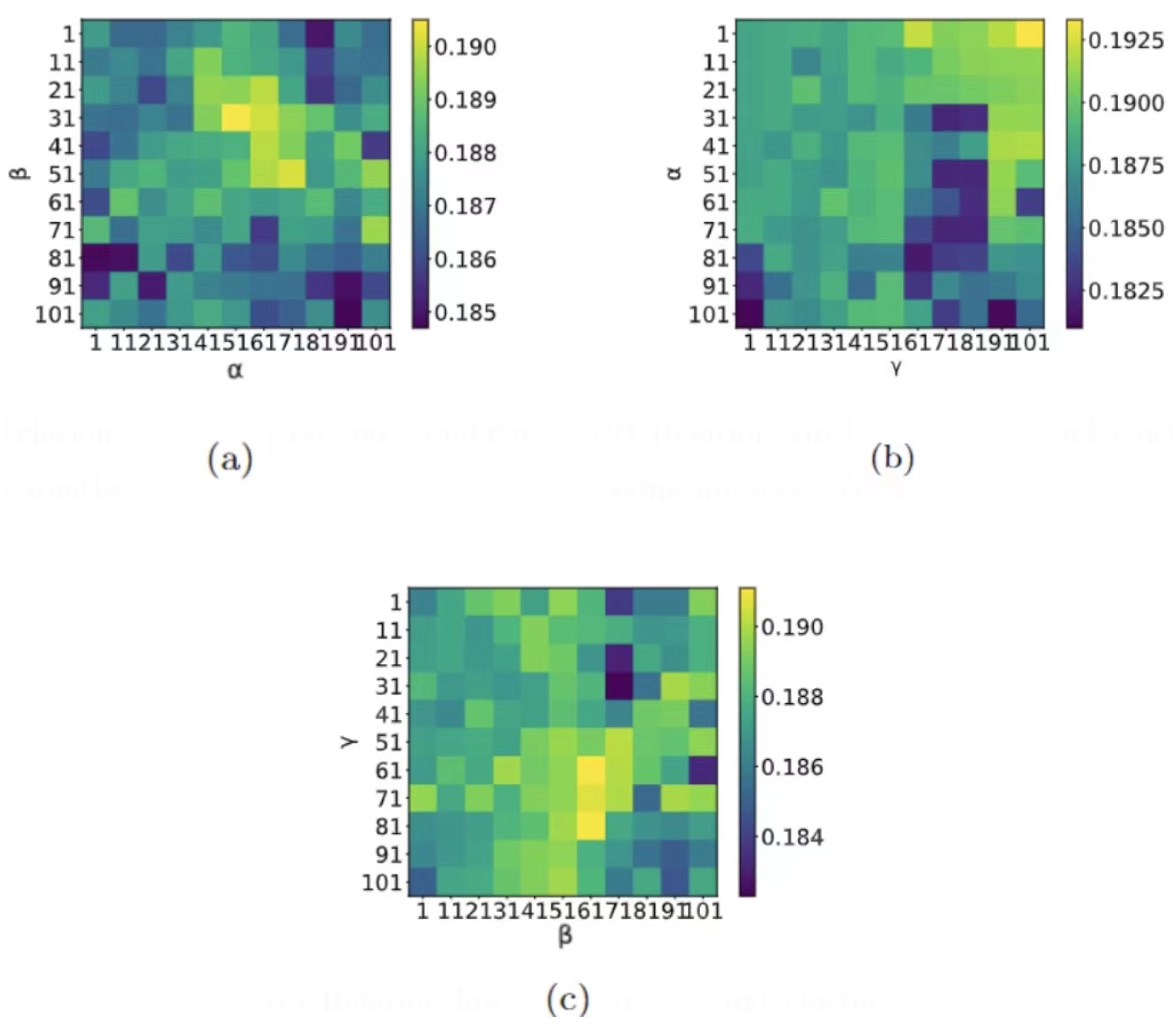
4.3. Parameter Sensitivity Analysis

This section analyzes the effects of parameters α , β , γ , r 1 , r 2 and r 3 of the MSDA-NMF model on the clustering performance. These effects are on the real network, where r i , i { 1 , 2 , 3 } are the i-level embedding dimensions. To determine the specific parameters of the model, this paper first fixed all the other parameters except the two changing numbers based on the OAG data set. Second, the effect of each change is verified by adjusting the parameters of the two changes. This paper takes the OAG data set as an example to investigate influences of different parameters. The effects of each parameter are explored through varying parameters and simultaneously keeping the others fixed. For example, we observe the effect of α , β by changing α , β and fixing γ with r 1 , r 2 , r 3 and so on. Specifically, we change r i , r { 1 , 2 , 3 } from 100, 200, 300, 400, 500, and ask for r 3 < r 2 < r 1 .
Figure 2 shows the influence of dimensions r 1 , r 2 and r 3 embedded in different layers on the effects of the three data clustering classes. The lighter the color of the point in the figure is, the larger the NMI value under the point coordinates. The NMI value of the yellow point is the maximum, and the NMI value of the purple point is the minimum. The size of a point also indicates the NMI value of the point. The larger the point is, the greater the NMI value of the point.
Figure 3a–c shows the performance of the NMI as these parameters change.
From the figures, we can see that:
1. In Figure 2, when r 1 is approximately 200, r 2 is approximately 170 and r 3 is 150, NMI is the maximum. If r 2 is controlled and r 3 remains unchanged, NMI decreases with the increase of r 1 , and the dimension of r 3 is not lower, but the NMI value is higher.
2. In Figure 3a:
(1) When α is less than 30, and β is greater than 80 and less than 100, the model has the worst value of robustness.
(2) When α is greater than 40 and less than 80, the NMI value tends to be stable with an increase in β to less than 50.
(3) When α is greater than 50 and β is less than 30, the model can obtain better clustering performance at this time.
3. In Figure 3b, when y is in [ 1 , 61 ] , NMI does not change much, indicating that when γ is in [ 81 , 101 ] , and the clustering performance is relatively stable with increasing γ .
4. In Figure 3c, we notice that in a particular range, when both β and γ increase, NMI tends to be stable, while when γ and β are in the range [ 61 , 81 ] , NMI reaches its maximum value.
As for the relationship between α , β , γ and the cluster evaluation index NMI, experimental results show that when r 1 = 200 , r 2 = 170 and r 3 = 150 , at this point, more effective network structure features can be obtained, even in low-dimensional space. Therefore, we set the data in the following experiment when r 1 = 200 , r 2 = 170 and r 3 = 150 .

4.4. Multiclassification Experiment

Table 3 illustrates the experimental results.
In the HEP-TH dataset, the MSDA-NMF ( V 2 ) model has a micro result of 31.15 and a macro result of 17.01 , just slightly below the optimal values of 33.87 and 25.58 for all the comparative models, respectively, but the results of this model are better than all the other comparative models except for the optimal value. The MSDA-NMF ( V 3 ) model has a micro result of 35.7 , better than all comparative models and 1.83 higher than the AROPE model, which has the highest micro result among them. In the macro comparison, the macro result of this model of 19.02 is only slightly lower than the optimal value of 25.58 of the GAE model, but still performs better in the optimal value than the other comparative models.
The results of the multiclassification experiments of the MSDA-NMF ( V 2 ) and the MSDA-NMF ( V 2 ) are compared. In the HEP-TH dataset, the results of the MSDA-NMF ( V 2 ) model are lower than those of the three-layer model. It can be seen that the more intermediate levels there are in the classification experiments, the more effective the MSDA-NMF can be in the model. In other citation network data sets, OAG and HEP-PH, the performance of the three-layer models proposed in this paper is superior to other models.
In addition, the micro and macro data results of the MSDA-NMF ( V 2 ) model proposed in this paper also outperformed the other models in the HEP-PH dataset, and the macro indicators were higher than the comparison models in the OAG dataset. In the HEP-TH, OAG and HEP-PH data sets, the micro-F1 and macro-F1 multi-classification evaluation performance of MSDA-NMF is better than those of NetMF, GAE and other popular feature models. This proves the effectiveness of our network-embedding model.
What is special here is that the AREOP model performs better than the MSDA-NMF method for the micro-F1 and macro-F1 metrics in our comparison based on the Wikipedia data set. This is probably because Wikipedia is a dense word co-occurrence network, so a relatively low order is sufficient to characterize Wikipedia’s web structure. Therefore, the MSDA-NMF method based only on matrix decomposition performs poorly in the classification task on sparse data sets.

4.5. Node Clustering Experiment

In this section, the behavior of node clusters is assessed according to the normalized mutual information (NMI) of typical metrics. In this paper, we use real data (including Polbog, Livejournal and Orkut) to assess the clustering performance of the model on real data sets. The NMI varies from 0 to 1, with a larger value indicating better cluster performance. In experiments to verify the clustering effect of the model, the standard K-means algorithm is used. Because the initial value has a significant impact on the clustering result, the clustering should be repeated 50 times and its average value should be considered as the result.
Figure 4 demonstrates the clustering ability of nodes with related NMI. It can be seen from the figure that:
1. In the Polblog and Orkut data sets, MSDA-NMF ( V 2 ) and MSDA-NMF ( V 3 ) obtained better results based on NMI compared with all models. In particular, in the Polblog data set, the MSDA-NMF ( V 2 ) and MSDA-NMF ( V 3 ) modes also have a great advantage in NMI value compared with the best DeepWalk mode among the comparison modes. This is because our method integrates lower-order structural features and multi-layer features to capture diverse and comprehensive structural features of the network, and can obtain better NMI values in data sets with a lower number of categories.
2. The model in this paper also achieves better results in Orkut data sets with fewer categories. What is special here is that in the relatively high number of categories in the Livejournal data set, the NMI value obtained by this model is slightly lower than that obtained by the GAE model. The main reason for this is that GAE has the same convolution structure as GCN and is based on a variational autoencoder, so GAE has better robustness in link prediction for citation networks.
3. SDNE and LINE only retain the proximity between network nodes and cannot effectively preserve the community structure. Random walk-based DeepWalk and Node2VEC can better capture the second-order and higher-order similarity. Although AROPE can capture the similarity of different nodes and capture more global structure information as the length increases, the omission of community structure makes the algorithm ignore module information. But for the sparse network and the network without prominent community structure, the modularity of the NMF is constrained by the similarity of nodes to each other. Therefore, its performance is relatively low.
This paper also compares the performance of the MSDA-NMF model of three-layer NMF and the MSDA-NMF model of two-layer NMF in multiclassification experiments. The results show that the NMI values obtained by the MSDA-NMF ( V 3 ) model are higher than those obtained by the MSDA-NMF ( V 2 ) model in all data sets. This proves the validity of the MSDA-NMF ( V 3 ) model in network embedding.

4.6. Link Prediction Experiment

Link prediction mainly detects the accuracy of prediction by predicting which pairs of nodes may form edges and comparing them with the actually deleted edges. In the experiment, we randomly hide the 10 % , 20 % , 30 % , 40 % and 50 % edges as test data, and the other edges are connected. We use the remaining edges to train the robust results of node embedding vectors. We evaluated the effectiveness of our model based on typical AUC (Area Under A Curve) evaluation indexes.
To verify the validity of our proposed model, we first delete the 10 % edge on all network data sets. As shown in Table 4:
1. Compared with other algorithms, MSDA-NMF ( V 3 ) improves the prediction performance by 10 % compared to the optimal prediction model GAE and 64 % .
2. Compared to the worst prediction model, MSDA-NMF ( V 2 ) has a low prediction performance of compared to the optimal prediction model in the comparison model.
3. In the comparison data set of Orkut and GR-QC:
(1) The proposed MSDA-NMF ( V 2 ) and MSDA-NMF ( V 3 ) models obtained the optimal prediction results.
(2) However, in the GR-QC data set, the accuracy of the MSDA-NMF ( V 3 ) model was higher than that of the MSDA-NMF ( V 2 ).
What is remarkable here is that in the Polblog data set, none of the methods proposed in this paper can obtain the optimal prediction effect. As shown in Table 2, the Polblog data set has a small number of pairs of categories, which makes the model unable to obtain better prediction results in hierarchical operation.
Specifically, to further verify the influence of the proportion of training data on the model, this paper conducted tests through Livejournal and Orkut data. The results in Figure 5 show that our method has a certain superiority over all the mainstream methods for removing different parts of edges in the two data sets. Because networks have different structural characteristics, the remaining edge of the Livejournal data set is close to the optimal level at 90 % , and MSDA-NMF ( V 2 ) obtains prediction results similar to those of MSDA-NMF ( V 3 ). It can be seen that our method has an excellent performance in link prediction, indicating that network embedding results retain the structural characteristics of data sets.

5. Conclusions and Future Work

This paper introduces the multilayer structure NMF, a complex hierarchical structure to realize the characteristics of the input data by adding the regularization constraint for each layer, the essential feature of depicting feature transformation to obtain the data one by one, to further merge their depth due to the multilayer structure of the encoder MSDA NMF model. It can effectively improve the detection accuracy and prediction accuracy of social groups in the complex social management system. Eight popular models, NetMF, M-NMF, DeepWalk, Node2vec, LINE SDNE, AROPE and GAE were compared with eight real data sets to verify the robustness of the algorithm.
Although the proposed method (the data set presented in this paper) has a good detection effect, there are still some problems to be solved; for example, the results of the model are not optimal in the network with a large number of categories. Therefore, how to overcome the multistructure characteristics of multicategories in real networks and models simultaneously is the key to effectively improving the detection performance of the model in all data sets, and it is also challenging and necessary work [48]. We will take these factors into account in our future work.

Author Contributions

Conceptualization, W.Y.; data curation, X.L.; formal analysis, W.Y. and X.L.; investigation, G.X.; methodology, W.Y.; resources, X.L.; software, G.X.; validation, F.L.; writing—original draft, W.Y. and X.L.; writing—review and editing, X.L. and F.L. All authors have read and agreed to the published version of the manuscript.

Funding

This work is supported in part by the Key R&D program of Zhejiang Province (2022C01083), the National Natural Science Foundation of China (62102262, 62172297, 61902276) and the State Key Development Program of China (No. 2019YFB2101700, No. 2018YFB0804402).

Institutional Review Board Statement

Not applicable.

Informed Consent Statement

Informed consent was obtained from all subjects involved in the study.

Data Availability Statement

Not applicable.

Conflicts of Interest

The authors declare no conflict of interest.

Abbreviations

The following abbreviations are used in this manuscript:
MDPIMultidisciplinary Digital Publishing Institute
DOAJDirectory of open access journals
TLAThree letter acronym
LDLinear dichroism

References

  1. Maisog, J.M.; DeMarco, A.T.; Devarajan, K.; Young, S.; Fogel, P.; Luta, G. Assessing Methods for Evaluating the Number of Components in Non-Negative Matrix Factorization. Mathematics 2021, 9, 2840. [Google Scholar] [CrossRef] [PubMed]
  2. Lee, D.D.; Seung, S.H. Learning the parts of objects by non-negative matrix factorization. Nature 1999, 401, 788–791. [Google Scholar] [CrossRef]
  3. Cai, T.; Li, J.; Mian, A.S.; Li, R.; Yu, J.X. Target-aware Holistic Influence Maximization in Spatial Social Networks. IEEE Trans. Knowl. Data Eng. 2020, 34(4), 1–14. [Google Scholar] [CrossRef]
  4. Stai, E.; Kafetzoglou, S.; Tsiropoulou, E.E.; Papavassiliou, S. A holistic approach for personalization, relevance feedback & recommendation in enriched multimedia content. Multimed. Tools Appl. 2018, 77, 283–326. [Google Scholar]
  5. Lambiotte, R.; Rosvall, M.; Scholtes, I. From networks to optimal higher-order models of complex systems. Nat. Phys. 2019, 15, 313–320. [Google Scholar] [CrossRef] [PubMed]
  6. Cai, H.; Zheng, V.W.; Chang, C.C. A Comprehensive Survey of Graph Embedding: Problems, Techniques, and Applications. IEEE Trans. Knowl. Data Eng. 2018, 30, 1616–1637. [Google Scholar] [CrossRef] [Green Version]
  7. Shao, W.; Fang, B.; Pu, W.; Ren, M.; Yi, S. A new method of extracting FECG by BSS of sparse signal. Sheng wu yi xue gong cheng xue za zhi = J. Biomed. Eng. 2009, 26, 1206–1210. [Google Scholar]
  8. Fan, Z.; Lei, L.; Zhang, K.; Trajcevski, G.; Zhong, T. DeepLink: A Deep Learning Approach for User Identity Linkage. In Proceedings of the IEEE INFOCOM 2018—IEEE Conference on Computer Communications, Honolulu, HI, USA, 16–19 April 2018. [Google Scholar]
  9. Xu, G.; Bai, X.; Luo, N.N.X.; Cheng, L.; Zheng, X. SG-PBFT: A secure and highly efficient distributed blockchain PBFT consensus algorithm for intelligent Internet of vehicles. J. Parallel Distrib. Comput. 2022, 164, 1–11. [Google Scholar] [CrossRef]
  10. Févotte, C.; Idier, J. Algorithms for nonnegative matrix factorization with the β-divergence. Neural Comput. 2011, 23, 2421–2456. [Google Scholar] [CrossRef]
  11. Hoyer, P.O. Non-negative sparse coding. In Proceedings of the 12th IEEE Workshop on Neural Networks for Signal Processing, Valais, Switzerland, 4–6 September 2002; pp. 557–565. [Google Scholar]
  12. Ren, B.; Pueyo, L.; Zhu, G.B.; Debes, J.; Duchêne, G. Non-negative matrix factorization: Robust extraction of extended structures. Astrophys. J. 2018, 852, 104. [Google Scholar] [CrossRef] [Green Version]
  13. Jia, Y.; Liu, H.; Hou, J.; Kwong, S. Semisupervised adaptive symmetric non-negative matrix factorization. IEEE Trans. Cybern. 2020, 51, 2550–2562. [Google Scholar] [CrossRef]
  14. Huang, Y.; Yang, G.; Wang, K.; Liu, H.; Yin, Y. Robust Multi-feature Collective Non-Negative Matrix Factorization for ECG Biometrics. Pattern Recognit. 2021, 123, 108376. [Google Scholar] [CrossRef]
  15. Hinton, G.E.; Osindero, S.; Teh, Y.W. A fast learning algorithm for deep belief nets. Neural Comput. 2006, 18, 1527–1554. [Google Scholar] [CrossRef]
  16. Salakhutdinov, R.; Tenenbaum, J.B.; Torralba, A. Learning with hierarchical-deep models. IEEE Trans. Pattern Anal. Mach. Intell. 2012, 35, 1958–1971. [Google Scholar] [CrossRef] [PubMed] [Green Version]
  17. Zhou, S.; Chen, Q.; Wang, X. Fuzzy deep belief networks for semi-supervised sentiment classification. Neurocomputing 2014, 131, 312–322. [Google Scholar] [CrossRef]
  18. Ye, F.; Chen, C.; Zheng, Z. Deep autoencoder-like nonnegative matrix factorization for community detection. In Proceedings of the 27th ACM International Conference on Information and Knowledge Management, Torino, Italy, 22–26 October 2018; pp. 1393–1402. [Google Scholar]
  19. De Handschutter, P.; Gillis, N.; Siebert, X. Deep matrix factorizations. arXiv 2020, arXiv:2010.00380. [Google Scholar]
  20. Li, X.; Xu, G.; Tang, M. Community detection for multi-layer social network based on local random walk. J. Vis. Commun. Image Represent. 2018, 57, 91–98. [Google Scholar] [CrossRef]
  21. Cichocki, A.; Zdunek, R. Multilayer nonnegative matrix factorisation. Electron. Lett. 2006, 42, 947–948. [Google Scholar] [CrossRef] [Green Version]
  22. Cichocki, A.; Zdunek, R. Multilayer nonnegative matrix factorization using projected gradient approaches. Int. J. Neural Syst. 2007, 17, 431–446. [Google Scholar] [CrossRef] [Green Version]
  23. Song, H.A.; Lee, S.Y. Hierarchical data representation model-multi-layer NMF. arXiv 2013, arXiv:1301.6316. [Google Scholar]
  24. Rajabi, R.; Ghassemian, H. Spectral unmixing of hyperspectral imagery using multilayer NMF. IEEE Geosci. Remote. Sens. Lett. 2014, 12, 38–42. [Google Scholar] [CrossRef] [Green Version]
  25. Chen, L.; Chen, S.; Guo, X. Multilayer NMF for blind unmixing of hyperspectral imagery with additional constraints. Photogramm. Eng. Remote Sens. 2017, 83, 307–316. [Google Scholar] [CrossRef]
  26. Yuan, Y.; Zhang, Z.; Liu, G. A novel hyperspectral unmixing model based on multilayer NMF with Hoyer’s projection. Neurocomputing 2021, 440, 145–158. [Google Scholar] [CrossRef]
  27. Cao, S.; Lu, W.; Xu, Q. Deep neural networks for learning graph representations. In Proceedings of the AAAI Conference on Artificial Intelligence, Phoenix, AZ, USA, 12–17 February 2016; Volume 30. [Google Scholar]
  28. Wang, D.; Cui, P.; Zhu, W. Structural deep network embedding. In Proceedings of the 22nd ACM SIGKDD International Conference on Knowledge Discovery and Data Mining, San Francisco, CA, USA, 13–17 August 2016; pp. 1225–1234. [Google Scholar]
  29. Yang, D.; Wang, S.; Li, C.; Zhang, X.; Li, Z. From properties to links: Deep network embedding on incomplete graphs. In Proceedings of the 2017 ACM on Conference on Information and Knowledge Management, Singapore, 6–10 November 2017; pp. 367–376. [Google Scholar]
  30. Kipf, T.N.; Welling, M. Variational graph auto-encoders. arXiv 2016, arXiv:1611.07308. [Google Scholar]
  31. Hamilton, W.L.; Ying, R.; Leskovec, J. Inductive representation learning on large graphs. arXiv 2017, arXiv:1706.02216. [Google Scholar]
  32. Bengio, Y.; Courville, A.; Vincent, P. Representation learning: A review and new perspectives. IEEE Trans. Pattern Anal. Mach. Intell. 2013, 35, 1798–1828. [Google Scholar] [CrossRef] [PubMed]
  33. Trigeorgis, G.; Bousmalis, K.; Zafeiriou, S.; Schuller, B.W. A deep matrix factorization method for learning attribute representations. IEEE Trans. Pattern Anal. Mach. Intell. 2016, 39, 417–429. [Google Scholar] [CrossRef] [Green Version]
  34. Qiu, J.; Dong, Y.; Ma, H.; Li, J.; Wang, K.; Tang, J. Network embedding as matrix factorization: Unifying deepwalk, line, pte, and node2vec. In Proceedings of the Eleventh ACM International Conference on Web Search and Data Mining, Los Angeles, CA, USA, 5–9 February 2018; pp. 459–467. [Google Scholar]
  35. El-Shorbagy, M.A.; Omar, H.A.; Fetouh, T. Hybridization of Manta-Ray Foraging Optimization Algorithm with Pseudo Parameter Based Genetic Algorithm for Dealing Optimization Problems and Unit Commitment Problem. Mathematics 2022, 10, 2179. [Google Scholar] [CrossRef]
  36. Leskovec, J.; Kleinberg, J.; Faloutsos, C. Graph evolution: Densification and shrinking diameters. ACM Trans. Knowl. Discov. Data (TKDD) 2007, 1, 2. [Google Scholar] [CrossRef]
  37. Chaudhuri, K.; Chung, F.; Tsiatas, A. Spectral clustering of graphs with general degrees in the extended planted partition model. In Proceedings of the Conference on Learning Theory, JMLR Workshop and Conference Proceedings, Edinburgh, Scotland, 25–27 June 2012; pp. 35-1–35-23. [Google Scholar]
  38. Adamic, L.A.; Glance, N. The political blogosphere and the 2004 US election: Divided they blog. In Proceedings of the 3rd International Workshop on Link Discovery, Chicago, IL, USA, 21–25 August 2005; pp. 36–43. [Google Scholar]
  39. Yang, J.; Leskovec, J. Defining and evaluating network communities based on ground-truth. Knowl. Inf. Syst. 2015, 42, 181–213. [Google Scholar] [CrossRef] [Green Version]
  40. Toutanova, K.; Klein, D.; Manning, C.D.; Singer, Y. Feature-rich part-of-speech tagging with a cyclic dependency network. In Proceedings of the 2003 Human Language Technology Conference of the North American Chapter of the Association for Computational Linguistics, Edmonton, AB, Canada, 27 May–1 June 2003; pp. 252–259. [Google Scholar]
  41. Wang, X.; Cui, P.; Wang, J.; Pei, J.; Zhu, W.; Yang, S. Community preserving network embedding. In Proceedings of the AAAI Conference on Artificial Intelligence, San Francisco, CA, USA, 4–9 February 2017; Volume 31, pp. 203–209. [Google Scholar]
  42. Zhang, Z.; Cui, P.; Wang, X.; Pei, J.; Yao, X.; Zhu, W. Arbitrary-order proximity preserved network embedding. In Proceedings of the 24th ACM SIGKDD International Conference on Knowledge Discovery & Data Mining, London, UK, 19–23 August 2018; pp. 2778–2786. [Google Scholar]
  43. Perozzi, B.; Al-Rfou, R.; Skiena, S. Deepwalk: Online learning of social representations. In Proceedings of the 20th ACM SIGKDD International Conference on Knowledge Discovery and Data Mining, New York, NY, USA, 24–27 August 2014; pp. 701–710. [Google Scholar]
  44. Grover, A.; Leskovec, J. node2vec: Scalable feature learning for networks. In Proceedings of the 22nd ACM SIGKDD International Conference on Knowledge Discovery and Data Mining, San Francisco, CA, USA, 13–17 August 2016; pp. 855–864. [Google Scholar]
  45. Tang, J.; Qu, M.; Wang, M.; Zhang, M.; Yan, J.; Mei, Q. Line: Large-scale information network embedding. In Proceedings of the 24th International Conference on World Wide Web, Florence, Italy, 18–22 May 2015; pp. 1067–1077. [Google Scholar]
  46. Barcelona, U.D.; Sescelades, C. Comparing community structure identification. Radiology 2005, 9, P09008. [Google Scholar]
  47. Hanley, J.A.; Mcneil, B.J. A method of comparing the areas under receiver operating characteristic curves derived from the same cases. Radiology 1983, 148, 839–843. [Google Scholar] [CrossRef] [PubMed] [Green Version]
  48. Xu, G.; Dong, W.; Xing, J.; Lei, W.; Liu, J.; Gong, L.; Feng, M.; Zheng, X.; Liu, S. Delay-CJ: A novel cryptojacking covert attack method based on delayed strategy and its detection. Digit. Commun. Netw. 2022, in press. [CrossRef]
Figure 1. Framework diagram of the MSDA-NMF model.
Mathematics 10 02750 g001
Figure 2. Analysis of the embedding dimension relationship of different layers.
Mathematics 10 02750 g002
Figure 3. Relationship between α , γ , β and cluster evaluation index NMI. (a) Relationship between α , β and cluster evaluation index NMI; (b) Relationship between α , γ and cluster evaluation index NMI; (c) Relationship between γ , β and cluster evaluation index NMI.
Mathematics 10 02750 g003
Figure 4. Evaluation of node clustering performance based on NMI.
Mathematics 10 02750 g004
Figure 5. Changing the predictive performance of training data ratios.
Mathematics 10 02750 g005
Table 1. Symbol Description.
SymbolDefinition
A The adjacency matrix of graph G
r i Embedding dimension of layer I NMF
Z i Layer I auxiliary matrix
V i I layer embeds the eigenmatrix
B Random walk eigenmatrix
C Second order node similarity eigenmatrix
v o l ( G ) = i j A ij The capacity of figure G
Table 2. Data set network structure information.
Data SetNumber of Nodes | V | Number of Edges | E | Number of Categories kMore Labels
Wikipedia477718,41240yes
Polblog133516,6272no
Livejournal11,118396,46126no
Orkut99823,0506no
GR-QC19,30926,16942no
Hep-TH29,555352,8075yes
Hep-PH30,501347,26838yes
OAG13,89086,78419yes
Table 3. Performance evaluation of multi-label classification.
ModelHep-THOAGWikipediaHep-PH
MicroMacroMicroMacroMicroMacroMicroMacro
NetMF31.5414.8616.0112.1049.99.2523.875.43
M-NMF21.816.5318.3411.1348.137.9124.259.17
LINE23.7413.3211.949.5441.749.7325.178.32
DeepWalk29.3217.3812.0510.0935.089.3826.2112.43
AROPE33.8714.5119.6112.7852.8310.6915.3910.37
GAE27.1125.5816.6711.8550.4810.7524.6611.13
MSDA-NMF ( V 2 )31.1517.0115.6413.8850.539.3327.1414.27
MSDA-NMF ( V 3 )35.7019.0219.815.8350.288.3128.515.6
Table 4. Experimental results of link prediction.
Data SetPolblogOrkutLivejournalGR-QC
NetMF0.5250.6500.7890.795
M-NMF0.6720.8350.1510.843
DeepWalk0.4990.4870.4460.849
Node2vec0.4950.5160.5120.530
LINE0.4710.4700.5720.508
SDNE0.4600.5210.6310.513
AROPE0.6940.6460.7380.734
GAE0.8590.7920.9670.937
MSDA-NMF ( V 2 )0.6720.8910.9630.884
MSDA-NMF ( V 3 )0.7820.9120.9800.953
Publisher’s Note: MDPI stays neutral with regard to jurisdictional claims in published maps and institutional affiliations.

