Some New n-Point Ternary Subdivision Schemes without the Gibbs Phenomenon

Abstract

This paper is devoted to the construction and analysis of some new families of n-point ternary subdivision schemes. Some members of the families were adapted to the presence of discontinuities converging to limit functions without Gibbs oscillations. We present a numerical comparison where we check the theoretical properties.

1. Introduction

Subdivision schemes are used in CAGD since they are able to generate curves and surfaces from an initial set of control points. In past years, a great number of works have been published on linear subdivision schemes.

In this paper, we present some new n-point ternary families of subdivision schemes:

• $S_0$, a 2-point interpolatory family that generates a continuous limit function; this family can be considered ’generalized’ of the ternary 2-point subdivision scheme proposed in [1].
• $S_1$, a 3-point approximating family that gives a $C^1$ continuous limit function.
• $S_2$, a 3-point approximating family that has $C^2$ continuity of the limit function; this family can be considered ‘generalized’ of the ternary 3-point subdivision scheme proposed in [1], the ternary 3-point subdivision scheme defined in [2] (with $\mu =1/18$), and the ternary subdivision scheme presented in [3].

We also propose new family-approximating subdivision schemes:

• A 4-point family ($S_3$) that gives a $C^3$ continuous limit function;
• A 5-point family ($S_5$,) that has $C^5$ continuity of the limit function;
• A 6-point family ($S_6$) that generates the $C^6$ limit function.

We prove the convergence of the new family subdivision schemes; in order to study the reproduction polynomial property, we present an important theorem (Theorem 7) for the m-ary subdivision scheme and we apply it to the new ternary subdivision schemes. Moreover, we study the polynomial generation and the absence of the Gibbs oscillations on the limit functions near discontinuities of the new families, and we perform a numerical comparison considering the case of discontinuities on the initial data.

The constructions of the subdivision schemes are interesting because we generalize some existing schemes, giving more possibilities. Moreover, the theoretical properties derived for the new schemes are important in applications, such as CAGD and image processing.

2. Background

A ternary subdivision scheme is defined by

$$f_i^{k+1}={\displaystyle \sum _{j\in }}{a}_{i-3j}{f}_j^k,i\in ,k{\in }_{+},$$

(1)

where $a=a_i\in \mathbb{R},i\in$ is called the mask.

The general form of (1) can be written as

$$\begin{array}{cc}\hfill f_{3i}^{k+1}=& {\displaystyle \sum _{j\in }}{a}_{3j}{f}_{i-j}^k,\hfill \\ \hfill f_{3i+1}^{k+1}=& {\displaystyle \sum _{j\in }}{a}_{3j+1}{f}_{i-j}^k,\hfill \\ \hfill f_{3i+2}^{k+1}=& {\displaystyle \sum _{j\in }}{a}_{3j+2}{f}_{i-j}^k.\hfill \end{array}$$

The norm ${\parallel .\parallel }_{\infty }$ of a ternary subdivision scheme S is defined by:

$${\parallel S\parallel }_{\infty }=max\left\{{\displaystyle \sum _i}|a_{3i}|,{\displaystyle \sum _i}|a_{3i+1}|,{\displaystyle \sum _i}|a_{3i+2}|\right\},$$

and the Laurent polynomial by

$$a\left(z\right)={\displaystyle \sum _{i\in }}{a}_i{z}^i.$$

For the convergence, we have the following results:

Definition 1

([4]). A triadic subdivision scheme S is said to be convergent if

$$\forall f\in l^{\infty }\left(\right),\exists g\in C^0\left(\mathbb{R}\right)suchthat{\displaystyle \underset{k\to +\infty }{lim}\underset{n\in }{sup}}|{\left(S^{k}f\right)}_n-g\left(3^{-k}n\right)|=0.$$

The limit function g is denoted by $g=S^{\infty }f.$

The next theorem presents a necessary condition for the convergence of a ternary subdivision scheme.

Theorem 1

([5]). Let S be a convergent ternary subdivision scheme, with a mask a. Then

$${\displaystyle \sum _n}{a}_{3n}={\displaystyle \sum _n}{a}_{3n+1}={\displaystyle \sum _n}{a}_{3n+2}=1.$$

(2)

The Laurent polynomial of a convergent ternary subdivision scheme verifies [6]

$$a(e^{2i\pi /3})=a(e^{4i\pi /3})=0\mathrm{and}a(1)=3,$$

and there exists the Laurent polynomial $a_1\left(z\right)$, such that

$$a_1\left(z\right)={\displaystyle \frac{3z^2}{1+z+z^2}}a\left(z\right).$$

The subdivision scheme $S_1$ (the first-order difference scheme of S) associates the symbol $a_1\left(z\right)$ and satisfies the following proposition:

Proposition 1

([6]). Let S be a subdivision scheme defined by a mask satisfying (2). Then there exists a subdivision scheme $S_1$ with the property

$$dS{f}^k=S_{1}d{f}^k,$$

where $f^k=S^k{f}^0,$ and ${\left(d{f}^k\right)}_i=3^k(f_{i+1}^k-f_i^k)$.

To prove the convergence of the subdivision scheme S, we use the subdivision scheme $S_1$ as follows:

Theorem 2

([5]). S is a uniformly convergent ternary subdivision scheme if and only if $\frac{1}{3}{S}_1$ converges uniformly to the zero function for all initial data $f^0$; that is

$${\displaystyle \underset{k\to \infty }{lim}}{(\frac{1}{3}{S}_1)}^k{f}^0=0.$$

(3)

According to Theorem 2, to prove that the convergence of S is equivalent to proving that $\parallel {\left(\frac{1}{3}{S}_1\right)}^L{\parallel }_{\infty }<1,$ for some integer $L>0$ (which means $\frac{1}{3}S$ is contractive), in this paper, we take $L=1$.

In order to check the regularity of the limit functions obtained by the subdivision scheme S, we apply the flowing theorem.

Theorem 3

([5]). Let us consider a scheme S with the Laurent polynomial $a\left(z\right)$. If there exists a polynomial $b\left(z\right)$, such that

$$a\left(z\right)={\left({\displaystyle \frac{1+z+z^2}{3z^2}}\right)}^{m}b\left(z\right),$$

(4)

and it is verified that the associated scheme $\frac{1}{3}{S}_b$ is contractive, then the limit function is $C^m$ for any initial data.

Corollary 1.

If there exists a polynomial $b\left(z\right)$, such that

$$a\left(z\right)={\left({\displaystyle \frac{1+z+z^2}{3z^2}}\right)}^{m+1}b\left(z\right),$$

(5)

with $\parallel {\left(\frac{1}{3}{S}_b\right)}^L{\parallel }_{\infty }<1,$ for some integer $L>0$, then the limit function is $C^m$ for any initial data.

Proof. 

We suppose that there exists a polynomial $b\left(z\right)$, verifying

$$\begin{array}{cc}\hfill a\left(z\right)=& {\left({\displaystyle \frac{1+z+z^2}{3z^2}}\right)}^{m+1}b\left(z\right)\hfill \\ \hfill =& {\left({\displaystyle \frac{1+z+z^2}{3z^2}}\right)}^m{\displaystyle \frac{1+z+z^2}{3z^2}}b\left(z\right)\hfill \\ \hfill =& {\left({\displaystyle \frac{1+z+z^2}{3z^2}}\right)}^{m}c\left(z\right),\hfill \end{array}$$

where $c\left(z\right)={\displaystyle \frac{1+z+z^2}{3z^2}}b\left(z\right)$, $\frac{1}{3}{S}_c$ is contractive. In fact, the symbol of the first-order difference scheme of $S_c$ is $c_1\left(z\right)=\frac{3z^2}{1+z+z^2}c\left(z\right)=b\left(z\right),$ then $S_b=S_{c1}\Rightarrow \parallel {\left(\frac{1}{3}{S}_{c1}\right)}^L\parallel =\parallel {\left(\frac{1}{3}{S}_b\right)}^L\parallel <1$, so $\frac{1}{3}{S}_c$ is contractive. □

3. Some New Families of n-Point Ternary Subdivision Schemes

In this section, we propose some new families of n-point ternary subdivision schemes with the parameter w. Firstly, we present the following new family of Laurent polynomials:

$$a_{\alpha }\left(z\right)={\displaystyle \frac{1}{3^{\alpha }}}{\displaystyle \frac{{(1+z+z^2)}^{\alpha +1}}{z^m}}\left\{\omega +(1-2w)z+w{z}^2\right\}$$

(6)

$\alpha =0,1,\dots ,6\dots$, where the exponents m depend on $\alpha$ and are given in the following table

$\alpha$	0	1	2	3	4	5	6
m	2	1	3	5	6	6	8

3.1. The 2-Point Ternary Interpolatory Subdivision Schemes

• A family of 2-point ternary interpolatory subdivision schemes can be obtained, after setting $\alpha =0$ in (6). We obtain the following Laurent polynomial:

$$\begin{array}{cc}\hfill a_0\left(z\right)=& {\displaystyle \frac{(1+z+z^2)}{z^2}}\left\{w+(1-2w)z+w{z}^2\right\}\hfill \\ \hfill =& w{z}^2+(1-w)z+1+(1-w)z^{-1}+w{z}^{-2}.\hfill \end{array}$$

(7)

The subdivision scheme $S_0$ associated with the Laurent polynomial (7) is the interpolating subdivision scheme:

$$\left\{\begin{array}{ccc}{f}_{3n}^{k+1}\hfill & =\hfill & f_n^k,\hfill \\ f_{3n+1}^{k+1}\hfill & =\hfill & (1-w)f_n^k+w{f}_{n+1}^k,\hfill \\ f_{3n+2}^{k+1}\hfill & =\hfill & w{f}_n^k+(1-w)f_{n+1}^k.\hfill \end{array}\right.$$

(8)

Remark 1.

For $w={\displaystyle \frac{1}{3}}$, this scheme coincides with the scheme by M.F. Hassan and N.A. Dodgson [1].

3.2. Two New Families of the 3-Point Ternary Subdivision Scheme

• Putting $\alpha =1$ in (6), we obtain the Laurent polynomial:

$$\begin{array}{cc}\hfill a_1\left(z\right)=& {\displaystyle \frac{1}{3}}{\displaystyle \frac{{(1+z+z^2)}^2}{z}}\left\{w+(1-2w)z+w{z}^2\right\}\hfill \\ \hfill =& {\displaystyle \frac{1}{3}}\{w{z}^5+z^4+2z^3+(3-2w)z^2+2z+1+w{z}^{-1}\}.\hfill \end{array}$$

(9)

The subdivision scheme $S_1$ corresponding to the Laurent polynomial (9) is:

$$\left\{\begin{array}{ccc}{f}_{3n}^{k+1}\hfill & =\hfill & {\displaystyle \frac{2}{3}}{f}_{n-1}^k+{\displaystyle \frac{1}{3}}{f}_n^k,\hfill \\ f_{3n+1}^{k+1}\hfill & =\hfill & {\displaystyle \frac{1}{3}}{f}_{n-1}^k+{\displaystyle \frac{2}{3}}{f}_n^k,\hfill \\ f_{3n+2}^{k+1}\hfill & =\hfill & {\displaystyle \frac{w}{3}}{f}_{n-1}^k+{\displaystyle \frac{(3-2w)}{3}}{f}_n^k+{\displaystyle \frac{w}{3}}{f}_{n+1}^k.\hfill \end{array}\right.$$

(10)

• For $\alpha =2$ in (6), we obtain the following Laurent polynomial:

$$\left\{\begin{array}{ccc}{a}_2\left(z\right)\hfill & =\hfill & {\displaystyle \frac{1}{9}}{\displaystyle \frac{{(1+z+z^2)}^3}{z^3}}\left\{w+(1-2w)z+w{z}^2\right\}\hfill \\ \hfill & =\hfill & {\displaystyle \frac{1}{9}}\{w{z}^5+(1+w)z^4+(3+w)z^3+(6-2w)z^2+(7-2w)z+(6-2w)\hfill \\ \hfill & \hfill & +(3+w)z^{-1}+(1+w)z^{-2}+w{z}^{-3}\}.\hfill \end{array}\right.$$

The subdivision scheme $S_2$ associated with the Laurent polynomial (11) is given as:

$$\left\{\begin{array}{ccc}{f}_{3n}^{k+1}\hfill & =\hfill & {\displaystyle \frac{3+w}{9}}{f}_{n-1}^k+{\displaystyle \frac{6-2w}{9}}{f}_n^k+{\displaystyle \frac{w}{9}}{f}_{n+1}^k,\hfill \\ f_{3n+1}^{k+1}\hfill & =\hfill & {\displaystyle \frac{1+w}{9}}{f}_{n-1}^k+{\displaystyle \frac{(7-2w)}{9}}{f}_n^k+{\displaystyle \frac{1+w}{9}}{f}_{n+1}^k,\hfill \\ f_{3n+2}^{k+1}\hfill & =\hfill & {\displaystyle \frac{w}{9}}{f}_{n-1}^k+{\displaystyle \frac{(6-2w)}{9}}{f}_n^k+{\displaystyle \frac{3+w}{9}}{f}_{n+1}^k.\hfill \end{array}\right.$$

(11)

Remark 2.

 

• For $w=-\frac{1}{2}$, the scheme coincides with the scheme by K. Rehan and S. Siddiqi, [2] (with $\mu =1/18$).

• For $w=\frac{1}{8}$, the above scheme coincides with the scheme by S. Siddiqi and K. Rehan, [3].

• For $w=\frac{1}{3}$, this scheme coincides with the scheme by M.F. Hassan and N.A. Dodgson, [1].

3.3. A New Family of 4-Point Ternary Subdivision Schemes

• We set $\alpha =3$ in (6), and obtain the Laurent polynomial:

$$\begin{array}{cc}\hfill a_3\left(z\right)=& {\displaystyle \frac{1}{3^3}}{\displaystyle \frac{{(1+z+z^2)}^4}{z^5}}\left\{w+(1-2w)z+w{z}^2\right\}\hfill \\ \hfill =& {\displaystyle \frac{1}{27}}\{w{z}^5+(1+2w)z^4+(4+3w)z^3+\left(10\right)z^2+(16-3w)z+(19-6w)\hfill \\ \hfill & +(16-3w)z^{-1}+10z^{-2}+(4+3w)z^{-3}+(1+2w)z^{-4}+w{z}^{-5}\}.\hfill \end{array}$$

(12)

The subdivision scheme $S_3$ associated with the Laurent polynomial (12) is:

$$\left\{\begin{array}{ccc}{f}_{3n}^{k+1}\hfill & =\hfill & {\displaystyle \frac{4+3w}{27}}{f}_{n-1}^k+{\displaystyle \frac{(19-6w)}{27}}{f}_n^k+{\displaystyle \frac{4+3w}{27}}{f}_{n+1}^k,\hfill \\ f_{3n+1}^{k+1}\hfill & =\hfill & {\displaystyle \frac{1+2w}{27}}{f}_{n-1}^k+{\displaystyle \frac{16-3w}{27}}{f}_n^k+{\displaystyle \frac{10}{27}}{f}_{n+1}^k+{\displaystyle \frac{w}{27}}{f}_{n+2}^k,\hfill \\ f_{3n+2}^{k+1}\hfill & =\hfill & {\displaystyle \frac{w}{27}}{f}_{n-1}^k+{\displaystyle \frac{10}{27}}{f}_n^k+{\displaystyle \frac{16-3w}{27}}{f}_{n+1}^k+{\displaystyle \frac{1+2w}{27}}{f}_{n+2}^k.\hfill \end{array}\right.$$

(13)

3.4. A New Family of 5-Point Ternary Subdivision Schemes

• For $\alpha =4$ in (6), we obtain the Laurent polynomial:

$$\begin{array}{cc}\hfill a_4\left(z\right)=& {\displaystyle \frac{1}{3^4}}{\displaystyle \frac{{(1+z+z^2)}^5}{z^6}}\left\{w+(1-2w)z+w{z}^2\right\}\hfill \\ \hfill =& {\displaystyle \frac{1}{81}}\{w{z}^6+(1+3w)z^5+(5+6w)z^4+(15+5w)z^3+\left(30\right)z^2+(45-9w)z\hfill \\ \hfill & +(51-12w)+(45-9w)z^{-1}+30z^{-2}+(15+5w)z^{-3}\hfill \\ & +(5+6w)z^{-4}+(1+3w)z^{-5}+w{z}^{-6}\}.\hfill \end{array}$$

(14)

The subdivision scheme $S_4$ associated with the Laurent polynomial (14) is:

$$\left\{\begin{array}{ccc}{f}_{3n}^{k+1}\hfill & =\hfill & {\displaystyle \frac{w}{81}}{f}_{n-2}^k+{\displaystyle \frac{15+5w}{81}}{f}_{n-1}^k+{\displaystyle \frac{51-12w}{81}}{f}_n^k+{\displaystyle \frac{15+5w}{81}}{f}_{n+1}^k+{\displaystyle \frac{w}{81}}{f}_{n+2}^k,\hfill \\ f_{3n+1}^{k+1}\hfill & =\hfill & {\displaystyle \frac{5+6w}{81}}{f}_{n-1}^k+{\displaystyle \frac{45-9w}{81}}{f}_n^k+{\displaystyle \frac{30}{81}}{f}_{n+1}^k+{\displaystyle \frac{1+3w}{81}}{f}_{n+2}^k,\hfill \\ f_{3n+2}^{k+1}\hfill & =\hfill & {\displaystyle \frac{1+3w}{81}}{f}_{n-1}^k+{\displaystyle \frac{30}{81}}{f}_n^k+{\displaystyle \frac{45-9w}{81}}{f}_{n+1}^k+{\displaystyle \frac{5+6w}{81}}{f}_{n+2}^k.\hfill \end{array}\right.$$

(15)

Remark 3.

 

• For $w=\frac{-5}{3}$, the above subdivision scheme $S_4$ coincides with the scheme of [7] (with $\mu =5/243$).

• This is exactly the same subdivision scheme defined in [8], where $w=-\frac{81}{a}$, (with $b=7a$, $c=6a$ and $d=3a$).

• For $\alpha =5$ in (6), we obtain the Laurent polynomial:

$$\begin{array}{cc}\hfill a_5\left(z\right)=& {\displaystyle \frac{1}{3^5}}{\displaystyle \frac{{(1+z+z^2)}^6}{z^6}}\left\{w+(1-2w)z+w{z}^2\right\}\hfill \\ \hfill =& {\displaystyle \frac{1}{243}}\{w{z}^8+(1+4w)z^7+(6+10w)z^6+(21+14w)z^5+(50+11w)z^4\hfill \\ \hfill & +(90-4w)z^3+(126-21w)z^2+(141-30w)z+126-21w+(90-4w)z^{-1}\hfill \\ & +(50+11w)z^{-2}+(21+14w)z^{-3}+(6+10w)z^{-4}+(1+4w)z^{-5}+w{z}^{-6}\}.\hfill \end{array}$$

(16)

The subdivision scheme $S_5$ associated with the Laurent polynomial (16) is:

$$\left\{\begin{array}{ccc}{f}_{3n}^{k+1}\hfill & =\hfill & {\displaystyle \frac{6+10w}{243}}{f}_{n-2}^k+{\displaystyle \frac{90-4w}{243}}{f}_{n-1}^k+{\displaystyle \frac{126-21w}{243}}{f}_n^k+{\displaystyle \frac{21+14w}{243}}{f}_{n+1}^k+{\displaystyle \frac{w}{243}}{f}_{n+2}^k,\hfill \\ f_{3n+1}^{k+1}\hfill & =\hfill & {\displaystyle \frac{1+4w}{243}}{f}_{n-2}^k+{\displaystyle \frac{50+11w}{243}}{f}_{n-1}^k+{\displaystyle \frac{141-30w}{243}}{f}_n^k+{\displaystyle \frac{50+11w}{243}}{f}_{n+1}^k+{\displaystyle \frac{1+4w}{243}}{f}_{n+2}^k,\hfill \\ f_{3n+2}^{k+1}\hfill & =\hfill & {\displaystyle \frac{w}{243}}{f}_{n-2}^k+{\displaystyle \frac{21+14w}{243}}{f}_{n-1}^k+{\displaystyle \frac{126-21w}{243}}{f}_n^k+{\displaystyle \frac{90-4w}{243}}{f}_{n+1}^k+{\displaystyle \frac{6+10w}{243}}{f}_{n+2}^k.\hfill \end{array}\right.$$

(17)

3.5. A New Family of 6-Point Ternary Subdivision Schemes

For $\alpha =6$ in (6), we obtain the Laurent polynomial:

$$\begin{array}{cc}\hfill a_6\left(z\right)=& {\displaystyle \frac{1}{3^6}}{\displaystyle \frac{{(1+z+z^2)}^7}{z^8}}\left\{w+(1-2w)z+w{z}^2\right\}\hfill \\ \hfill =& {\displaystyle \frac{1}{729}}\{w{z}^8+(1+5w)z^7+(7+15w)z^6+(28+28w)z^5+(77+35w)z^4+(161+21w)z^3\hfill \\ \hfill & +(266-14w)z^2+(357-55w)z+(393-72w)+(357-55w)z^{-1}+(266-14w)z^{-2}\hfill \\ & +(161+21w)z^{-3}+(77+35w)z^{-4}+(28+28w)z^{-5}+(7+15w)z^{-6}+(1+5w)z^{-7}\hfill \\ \hfill & +\left(w\right)z^{-8}\}.\hfill \end{array}$$

(18)

The subdivision scheme $S_6$ associated with the Laurent polynomial (18) is:

$$\left\{\begin{array}{ccc}{f}_{3n}^{k+1}\hfill & =\hfill & {\displaystyle \frac{7+15w}{729}}{f}_{n-2}^k+{\displaystyle \frac{161+21w}{729}}{f}_{n-1}^k+{\displaystyle \frac{393-72w}{729}}{f}_n^k+{\displaystyle \frac{161+21w}{729}}{f}_{n+1}^k+{\displaystyle \frac{7+15w}{729}}{f}_{n+2}^k,\hfill \\ f_{3n+1}^{k+1}\hfill & =\hfill & {\displaystyle \frac{1+5w}{729}}{f}_{n-2}^k+{\displaystyle \frac{77+35w}{729}}{f}_{n-1}^k+{\displaystyle \frac{357-55w}{729}}{f}_n^k+{\displaystyle \frac{266-14w}{729}}{f}_{n+1}^k+{\displaystyle \frac{28+28w}{729}}{f}_{n+2}^k+{\displaystyle \frac{w}{729}}{f}_{n+3}^k,\hfill \\ f_{3n+2}^{k+1}\hfill & =\hfill & {\displaystyle \frac{w}{729}}{f}_{n-2}^k+{\displaystyle \frac{28+28w}{729}}{f}_{n-1}^k+{\displaystyle \frac{266-14w}{729}}{f}_n^k+{\displaystyle \frac{357-55w}{729}}{f}_{n+1}^k+{\displaystyle \frac{77+35w}{729}}{f}_{n+2}^k+{\displaystyle \frac{1+5w}{729}}{f}_{n+3}^k,\hfill \end{array}\right.$$

(19)

4. Convergence Analysis

Theorem 4.

The families of ternary subdivision schemes $S_{\alpha }$, defined in (8), (10), (11), (13), (15), (17), and (19) converge when $w\in ]0,1[$, $]-1,2[$, $]-3/2,3[$, $]-11/2,15/2[$, $]-35/6,23/3[$, $]-37/4,11[$ and $]-54/5,64/5[$, respectively.

Proof. 

The family of Laurent polynomials (6) can be written as

$$a_{\alpha }\left(z\right)=\left({\displaystyle \frac{1+z+z^2}{3z^2}}\right)b_{\alpha }\left(z\right),$$

where

$$b_{\alpha }\left(z\right)=3^{1-\alpha }{z}^{2-m}{(1+z+z^2)}^{\alpha }\{w+(1-2w)z+w{z}^2\}.$$

($b_{\alpha }\left(z\right)$ is the symbol of the first-order difference of the scheme $S_{\alpha }$).

Case 1: if $\alpha =0$, then

$b_0\left(z\right)=3\{w+(1-2w)z+w{z}^2\},$ we have the mask of the scheme $S_{b_0}$, $b_0^{\prime }=\{3w,3(1-2w),3w\}.$ Since $\parallel \frac{1}{3}{S}_{b_0}{\parallel }_{\infty }=max\left\{\right|w|,|1-2w\left|\right\}$, this norm $\parallel \frac{1}{3}{S}_{b_0}{\parallel }_{\infty }<1$, when $w\in ]0,1[$.

Case 2: if $\alpha =1$, then

$$b_1\left(z\right)=\{w{z}^5+(1-w)z^4+z^3+(1-w)z^2+wz\},$$

we have the mask of the scheme $S_{b_1}$

$$b_1^{\prime }=\{w,(1-w),1,(1-w),w\}.$$

Since $\parallel \frac{1}{3}{S}_{b_1}{\parallel }_{\infty }=\frac{1}{3}max\left\{\right|w|+|1-w|,1\}$, this norm $\parallel \frac{1}{3}{S}_{b_1}{\parallel }_{\infty }<1$, when $w\in ]-1,2[$.

Case 3: $\alpha =2$, in this case

$$b_2\left(z\right)=\frac{1}{3}\{w{z}^5+z^4+2z^3+(3-2w)z^2+2z+1+w{z}^{-1}\},$$

we have the mask of the scheme $S_{b_2}$

$$b_2^{\prime }=\frac{1}{3}\{w,1,2,(3-2w),2,1,w\}.$$

Since $\parallel \frac{1}{3}{S}_{b_2}{\parallel }_{\infty }=\frac{1}{9}max\left\{2\right|w|+|3-2w|,3\}$, this norm $\parallel \frac{1}{3}{S}_{b_2}{\parallel }_{\infty }<1$, when $w\in ]-3/2,3[$.

Case 4: for $\alpha =3$, we have

$$b_3\left(z\right)=\frac{1}{3^2}\{w{z}^5+(1+w)z^4+(3+w)z^3+(6-2w)z^2+(7-2w)z+(6-2w)+(3+w)z^{-1}+(1+w)z^{-2}+\left(w\right)z^{-3}\},$$

we have the mask of the scheme $S_{b_3}$

$$b_3^{\prime }=\frac{1}{3^2}\{w,1+w,3+w,6-2w,7-2w,6-2w,3+w,1+w,w\}.$$

Since $\parallel \frac{1}{3}{S}_{b_3}{\parallel }_{\infty }=\frac{1}{27}max\left\{\right|w|+|6-2w|+|3+w|,|1+w|+|7-2w|+|1+w\left|\right\}$, this norm $\parallel \frac{1}{3}{S}_{b_3}{\parallel }_{\infty }<1$, when $w\in ]-11/2,15/2[$.

Case 5: if $\alpha =4$, then

$b_4\left(z\right)=\frac{1}{3^3}\{w{z}^6+(1+2w)z^5+(4+3w)z^4+\left(10\right)z^3+(16-3w)z^2+(19-6w)z+(16-3w)+\left(10\right)z^{-1}+(4+3w)z^{-2}+(1+2w)z^{-3}+\left(w\right)z^{-4}\},$ we have the mask of the scheme $S_{b_4}$

$$b_4^{\prime }=\frac{1}{27}\{w,1+2w,4+3w,10,16-3w,19-6w,16-3w,10,4+3w,1+2w,w\}.$$

Since $\parallel \frac{1}{3}{S}_{b_4}{\parallel }_{\infty }=\frac{1}{81}max\left\{\right|w|+10+|16-3w|+|1+2w|,2|4+3w|+|19-6w\left|\right\}$, this norm $\parallel \frac{1}{3}{S}_{b_3}{\parallel }_{\infty }<1$, when $w\in ]-35/6,23/3[$.

Case 6: if $\alpha =5$, then

$b_5\left(z\right)=\frac{1}{3^4}\{w{z}^8+(1+3w)z^7+(5+6w)z^6+(15+5w)z^5+\left(30\right)z^4+(45-9w)z^3+(51-12w)z^2+(45-9w)z+\left(30\right)+(15+5w)z^{-1}+(5+6w)z^{-2}+(1+3w)z^{-3}+\left(w\right)z^{-4}\},$ the mask of the scheme $S_{b_5}$ is

$b_5^{\prime }=\frac{1}{81}\{w,1+3w,5+6w,15+5w,30,45-9w,51-12w,45-9w,30,15+5w,5+6w,1+3w,w\}.$

Since $\parallel \frac{1}{3}{S}_{b_5}{\parallel }_{\infty }=\frac{1}{243}max\left\{2\right|w|+2|15+5w|+|51-12w|,|1+3w|+30+|45-9w|+|5+6w\left|\right\}$, this norm $\parallel \frac{1}{3}{S}_{b_5}{\parallel }_{\infty }<1$, when $w\in ]-37/4,11[$.

Case 7: for $\alpha =6$,

$$b_6\left(z\right)=\frac{1}{3^5}\{w{z}^8+(1+4w)z^7+(6+10w)z^6+(21+14w)z^5+(50+11w)z^4+(90-4w)z^3+(126-21w)z^2+(141-30w)z+(126-21w)+(90-4w)z^{-1}+(50+11w)z^{-2}+(21+14w)z^{-3}+(6+10w)z^{-4}+(1+4w)z^{-5}+\left(w\right)z^{-6}\},$$

The norm $\parallel \frac{1}{3}{S}_{b_6}{\parallel }_{\infty }=\frac{1}{729}max\left\{\right|w|+|21+14w|+|126-21w|+|90-4w|+|6+10w|,|1+4w|+|50+11w|+|141-30w|+|50+11w|+|1+4w\left|\right\}$, this norm $\parallel \frac{1}{3}{S}_{b_6}{\parallel }_{\infty }<1$, when $w\in ]-54/5,64/5[$. □

Theorem 5.

The families of ternary subdivision schemes $S_{\alpha }$, defined in (8), (10), (11), (13), (15), (17), and (19) converge and have smoothness $C^{\alpha }$ when $w\in ]0,1[$.

Proof. 

The family of Laurent polynomials (6) can be written as

$$a_{\alpha }\left(z\right)={\left({\displaystyle \frac{1+z+z^2}{3z^2}}\right)}^{\alpha +1}{b}_{\alpha }\left(z\right),$$

where

$$b_{\alpha }\left(z\right)=3z^{2\alpha +2-m}\{w+(1-2w)z+w{z}^2\},$$

we have the mask of the scheme $S_{b_{\alpha }}$

$$b_{\alpha }^{\prime }=\{3w,3(1-2w),3w\}.$$

Since $\parallel \frac{1}{3}{S}_{b_{\alpha }}{\parallel }_{\infty }=max\left\{\right|w|,|1-2w\left|\right\}$, this norm $\parallel \frac{1}{3}{S}_{b_{\alpha }}{\parallel }_{\infty }<1$, when $w\in ]0,1[$.

Hence, the family of the subdivision scheme $S_{\alpha }$ is $C^{\alpha }$ when $w\in ]0,1[$. □

Hölder Regularity

Theorem 6.

The Hölder regularity of the families of ternary subdivision schemes $S_{\alpha }$, defined in (8), (10), (11), (13), (15), (17), and (19), respectively, is $R_H$, where

$$R_H=\left\{\begin{array}{cc}\alpha -{log}_3(1-2w),\hfill & if0<w<\frac{1}{3},\hfill \\ \alpha -{log}_3\left(w\right),\hfill & if\frac{1}{3}<w<1,\hfill \\ \alpha +1,\hfill & ifw=\frac{1}{3}.\hfill \end{array}\right.$$

Proof. 

The proof of the theorem (5) implies that

$$\parallel \frac{1}{3}{S}_{b_{\alpha }}{\parallel }_{\infty }=\left\{\begin{array}{cc}1-2w,\hfill & \mathrm{if}0<w<\frac{1}{3},\hfill \\ w,\hfill & \mathrm{if}\frac{1}{3}<w<1,\hfill \\ \frac{1}{3},\hfill & \mathrm{if}w=\frac{1}{3}.\hfill \end{array}\right.$$

Following the method of O. Rioul in [9], the ternary subdivision schemes $S_{\alpha }$, have a Hölder regularity $R_H=\alpha +v^k,\forall k\ge 1$, where v verifies

$$3^{-k{v}^k}=\parallel {({\displaystyle \frac{1}{3}}{S}_{b_{\alpha }})}^k{\parallel }_{\infty }.$$

Choosing $k=1$, we have

$$v=\left\{\begin{array}{cc}-{log}_3(1-2w)\hfill & \mathrm{if}0<w<\frac{1}{3},\hfill \\ -{log}_3\left(w\right)\hfill & \mathrm{if}\frac{1}{3}<w<1,\hfill \\ 1\hfill & \mathrm{if}w=\frac{1}{3}.\hfill \end{array}\right.$$

 □

5. Reproduction Polynomials of Any m-Arity Subdivision Scheme and Comparisons

To study the reproduction polynomials of the subdivision schemes, we need some results.

Definition 2

([10]). A subdivision scheme $S_a$ reproduces polynomials of degree d if it is convergent and if $S_a^{\infty }{f}^0=p$ for any polynomial $p\in {\pi }_d$ and initial data $f_i^0=p(t_i^0),i\in \mathbb{Z}.$

Let $m\ge 2$, the arity of a subdivision scheme and the subsymbols of a Laurent polynomial $a\left(z\right)$ are defined in [11] by

$$a_i\left(z\right)={\displaystyle \sum _{j\in \mathbb{Z}}}{a}_{mj+i}{z}^{mj+i},i=0,\dots ,m-1$$

and the k-th derivative of a subsymbol $a_i\left(z\right)$ is given as

$$a_i^{\left(k\right)}\left(z\right)={\displaystyle \sum _{j\in \mathbb{Z}}}{q}_{k,i}\left(j\right)a_{mj+i}{z}^{mj+i-k},$$

where $q_{k,i}\in {\mathbb{P}}_k$ are the polynomials

$$q_{k,i}\left(x\right)={\displaystyle \prod _{n=0}^{k-1}}(mx+i-n).$$

Lemma 1

([11]). The k-th derivative of a Laurent polynomial $a\left(z\right)$ satisfies

$$a^{\left(k\right)}\left({\zeta }_m^j\right)=0,j=1,\dots ,m-1,$$

if and only if

$$a_i^{\left(k\right)}\left(1\right)=a^{\left(k\right)}\left(1\right)/m,i=0,\dots ,m-1.$$

where ${\zeta }_m^j=exp\left(\frac{2\pi i}{m}j\right)$ are the m roots of the unity.

Corollary 2.

The k-th derivative of a Laurent polynomial $a\left(z\right)$ verifies

$$a^{\left(k\right)}\left({\zeta }_m^j\right)=0,j=1,\dots ,m-1,$$

if and only if

$${\displaystyle \sum _{j\in \mathbb{Z}}}{q}_{k,i}(-j)a_{i-mj}=a^{\left(k\right)}\left(1\right)/m,i=0,\dots m-1.$$

Proof. 

We first remark that

$$a_i^{\left(k\right)}\left(1\right)={\displaystyle \sum _{j\in \mathbb{Z}}}{q}_{k,i}\left(j\right)a_{mj+i}={\displaystyle \sum _{j\in \mathbb{Z}}}{q}_{k,i}(-j)a_{-mj+i},i=0,\dots ,m-1,$$

new we use the Lemma 1 to obtain the result. □

Lemma 2.

Let $d\in \mathbb{N}$ and $\tau \in \mathbb{R}$. Then a Laurent polynomial $a\left(z\right)$ satisfies

$${\displaystyle a^{\left(k\right)}\left(1\right)=m{\displaystyle \prod _{l=0}^{k-1}}(\tau -l)ifk=1,\dots ,d}$$

(20)

and

$$a^{\left(k\right)}\left({\zeta }_m^j\right)=0,j=1,\dots ,m-1,fork=1,\dots ,d,$$

(21)

if and only if

$${\displaystyle \sum _{j\in \mathbb{Z}}}{j}^k{a}_{i-mj}={\left(\frac{i-\tau }{m}\right)}^k,i=0,\dots m-1,fork=1,\dots ,d.$$

(22)

Proof. 

Using Corollary 2, we obtain equivalence between the conditions (20), (21) and

$${\displaystyle \sum _{j\in \mathbb{Z}}}{q}_{k,i}(-j)a_{i-mj}={\displaystyle \prod _{l=0}^{k-1}}(\tau -l),i=1,\dots ,m-1.$$

(23)

If $k=1$, using the definition of the polynomial $q_{1,i}$ and Relation (23), we have for any $i=1,\dots ,m-1$:

$$\begin{array}{cc}\hfill & {\displaystyle \sum _{j\in \mathbb{Z}}}{q}_{1,i}(-j)a_{i-mj}=\tau \hfill \\ \hfill \iff & {\displaystyle \sum _{j\in \mathbb{Z}}}(-jm+i)a_{i-mj}=\tau \hfill \\ \hfill \iff & -m{\displaystyle \sum _{j\in \mathbb{Z}}}j{a}_{i-mj}+i=\tau \hfill \\ \hfill \iff & {\displaystyle \sum _{j\in \mathbb{Z}}}j{a}_{i-mj}=\frac{i-\tau }{m}.\hfill \end{array}$$

Let us assume that there is an equivalence between (22) and (23) for $k=1,\dots ,d-1$ and we prove this equivalence for $k=d$.

Because the polynomial $q_{d,i}(-x)$ is of degree d, then $\exists {\gamma }_0,\dots ,{\gamma }_d\in \mathbb{R}$ with ${\gamma }_d\ne 0$, such that

$$q_{d,i}(-x)={\displaystyle \sum _{n=0}^d}{\gamma }_n{x}^n.$$

For $k=d$ and any $i=0,\dots ,m-1$

$$\begin{array}{cc}\hfill {\displaystyle \prod _{l=0}^{d-1}}(\tau -l)& ={\displaystyle \sum _{j\in \mathbb{Z}}}{q}_{d,i}(-j)a_{i-mj}={\displaystyle \sum _{j\in \mathbb{Z}}}\left({\displaystyle \sum _{n=0}^d}{\gamma }_n{j}^n\right)a_{i-mj}\hfill \\ & ={\gamma }_d{\displaystyle \sum _{j\in \mathbb{Z}}}{j}^d{a}_{i-mj}+{\displaystyle \sum _{n=0}^{d-1}}{\gamma }_n{\displaystyle \sum _{j\in \mathbb{Z}}}{j}^n{a}_{i-mj}\hfill \\ & ={\gamma }_d{\displaystyle \sum _{j\in \mathbb{Z}}}{j}^d{a}_{i-mj}+{\displaystyle \sum _{n=0}^{d-1}}{\gamma }_n{\left(\frac{i-\tau }{m}\right)}^n\hfill \\ & ={\gamma }_d{\displaystyle \sum _{j\in \mathbb{Z}}}{j}^d{a}_{i-mj}+q_{d,i}\left(\frac{\tau -i}{m}\right)-{\gamma }_d{\left(\frac{i-\tau }{m}\right)}^d\hfill \\ & ={\gamma }_d{\displaystyle \sum _{j\in \mathbb{Z}}}{j}^d{a}_{i-mj}-{\gamma }_d{\left(\frac{i-\tau }{m}\right)}^d+{\displaystyle \prod _{n=0}^{d-1}}(\tau -n).\hfill \end{array}$$

Since ${\gamma }_d\ne 0$, this is equivalent to

$${\displaystyle \sum _{j\in \mathbb{Z}}}{j}^d{a}_{i-mj}={\left(\frac{i-\tau }{m}\right)}^d.$$

 □

To present the main theorem in this section, we need a parameterization $\tau$ defined as following

Definition 3

([11]). For any subdivision scheme $S_a$, we denote by $\tau =a^{\prime }\left(1\right)/3$ the corresponding parametric shift and attach the data $f_n^k$ for $n\in ,k\in$ to the parameter values

$$x_n^k=x_0^k+\frac{n}{3^k}with{x}_0^k=x_0^{k-1}-\frac{\tau }{3^k}.$$

(24)

Theorem 7.

A convergent subdivision scheme $S_a$ with an arity $m\ge 2$ reproduces polynomials of degree $d\ge 1$ with respect to the parameterization in (24) if and only if

$${\displaystyle \sum _{j\in \mathbb{Z}}}{j}^k{a}_{mj+i}={\left(\frac{\tau -i}{m}\right)}^k,i=0,\dots ,m-1,fork=1,\dots ,d.$$

(25)

where $\tau =\frac{a^{\prime }\left(1\right)}{m}.$

Proof. 

It follows from Theorem 4.3 in [11] and Lemma (2). □

Remark 4.

The necessary condition for the convergence ${\displaystyle \sum _{i\in }{a}_{mi+l}=1,l=0,\dots ,m-1}$ imply the reproduction of the constants $(d=0)$.

Particular case.

For a ternary subdivision scheme ($m=3$), the relation (25) can be written as

$$\left\{\begin{array}{c}{\displaystyle \sum _{j\in }{j}^k{a}_{3j}={\left({\displaystyle \frac{\tau }{3}}\right)}^k,}\hfill \\ {\displaystyle \sum _{j\in }{j}^k{a}_{3j+1}={\left({\displaystyle \frac{\tau -1}{3}}\right)}^k,}\hfill \\ {\displaystyle \sum _{j\in }{j}^k{a}_{3j+2}={\left({\displaystyle \frac{\tau -2}{3}}\right)}^k.}\hfill \end{array}\right.$$

(26)

for $k=1,\dots ,d.$

5.1. Polynomial Reproduction and Approximation Order of the Subdivision Schemes

To obtain the order of approximation of the family subdivision schemes, we use the next theorem

Theorem 8

([12]). A convergent subdivision scheme that reproduces polynomial ${\mathbb{P}}_n$ has an approximation order of $n+1.$

Theorem 9.

The subdivision scheme $S_0$ defined by (8) reproduces the polynomial of degree 1 when $w=1/3$.

Proof. 

The first derivative of (7) at $z=1$, gives $a_0^{\prime }\left(1\right)=0$, so $\tau =0,$ then the system (26) becomes:

$$\left\{\begin{array}{cc}{a}_{-2}\hfill & ={\displaystyle \frac{1}{3^k}},\hfill \\ a_{-1}\hfill & ={\displaystyle \frac{2}{3^k}}.\hfill \end{array}\right.$$

(27)

because this system is verified only for $k=1$, we obtain the result. □

Corollary 3.

The interpolatory subdivision scheme defined in (8) has an approximation order of 2 when $w=\frac{1}{3}$.

Theorem 10.

The subdivision scheme $S_1$ defined by (10) reproduces the polynomial of degree 1 $\forall w\in ]-1,2[$.

Proof. 

After calculating the derivative of (9) and substituting $z=1$ in it, we have $a_1^{\prime }\left(1\right)=6$, so $\tau =2,$ then the system (26) becomes:

$$\left\{\begin{array}{cc}{a}_3\hfill & ={\left(\frac{2}{3}\right)}^k,\hfill \\ a_4\hfill & =\frac{1}{3^k},\hfill \\ a_5+{(-1)}^k{a}_{-1}\hfill & =0.\hfill \end{array}\right.$$

(28)

this system is verified for k = 1, $\forall w\in ]-1,2[$, then $S_1$ reproduces the polynomial of degree 1, $\forall w\in ]-1,2[$. □

Theorem 11.

The subdivision $S_2$, defined by (11) reproduces polynomials of degree 1 $\forall w\in ]-\frac{3}{2},3[$, and of degree 2 for $w=-1$.

Proof. 

The first derivative of (11) at $z=1$, gives $a_2^{\prime }\left(1\right)=3$, so $\tau =1,$ then the system (26) becomes:

$$\left\{\begin{array}{cc}{a}_3+{(-1)}^k{a}_{-3}\hfill & ={\left(\frac{1}{3}\right)}^k,\hfill \\ a_4+{(-1)}^k{a}_{-2}\hfill & =0,\hfill \\ a_5+{(-1)}^k{a}_{-1}\hfill & ={\left(\frac{-1}{3}\right)}^k,\hfill \end{array}\right.$$

since this system is verified for $k=1$, $\forall w\in ]-\frac{3}{2},3[$, and for $k=2,$ when $w=-1$, we obtain the result. □

Theorem 12.

The subdivision scheme $S_3$ defined in (13) reproduces the polynomial of degree 1 $\forall w\in ]-\frac{11}{2},\frac{15}{2}[$, and degree 2 when $w=\frac{-4}{3}$.

Proof. 

The first derivative of (12) at $z=1$, gives $a_3^{\prime }\left(1\right)=0$, so $\tau =0,$ then the system (26) becomes:

$$\left\{\begin{array}{cc}{a}_3+{(-1)}^k{a}_{-3}\hfill & =0,\hfill \\ a_4+{(-1)}^k{a}_{-2}+{(-2)}^k{a}_{-5}\hfill & ={\left(\frac{-1}{3}\right)}^k,\hfill \\ a_5+{(-1)}^k{a}_{-1}+{(-2)}^k{a}_{-4}\hfill & ={\left(\frac{-2}{3}\right)}^k.\hfill \end{array}\right.$$

(29)

the system (29) is verified for $k=1$, $\forall w\in ]-\frac{11}{2},\frac{15}{2}[$, and for $k=2,$ when $w=-4/3$, so we have the result. □

Theorem 13.

The subdivision scheme $S_4$ defined in (15) reproduces the polynomial of degree 1 $\forall w\in ]-\frac{-35}{6},\frac{23}{3}[$ and of degree 3 for $w=-5/3$.

Proof. 

The first derivative of (14) at $z=1$, gives $a_4^{\prime }\left(1\right)=0$, so $\tau =0,$ then the system (26) becomes:

$$\left\{\begin{array}{cc}\hfill 2^k{a}_6+a_3+{(-1)}^k{a}_{-3}+{(-2)}^k{a}_{-6}& =0,\hfill \\ \hfill a_4+{(-1)}^k{a}_{-2}+{(-2)}^k{a}_{-5}& ={\left(\frac{-1}{3}\right)}^k,\hfill \\ \hfill a_5+{(-1)}^k{a}_{-1}+{(-2)}^k{a}_{-4}& ={\left(\frac{-2}{3}\right)}^k,\hfill \end{array}\right.$$

(30)

since this system is verified for $k=1$, $\forall w\in ]-\frac{-35}{6},\frac{23}{3}[$, and for $k=2$ and 3, when $w=-5/3$, we have the result. □

Theorem 14.

The subdivision scheme $S_5$ defined by (17), reproduces the polynomial of degree 1 $\forall w\in ]-\frac{37}{4},11[$, and of degree 3 for $w=-2$.

Proof. 

The first derivative of (16) at $z=1$, gives $a_5^{\prime }\left(1\right)=3$, so $\tau =1,$ then the system (26) becomes:

$$\left\{\begin{array}{cc}{2}^k{a}_6+a_3+{(-1)}^k{a}_{-3}+{(-2)}^k{a}_{-6}\hfill & ={\left(\frac{1}{3}\right)}^k,\hfill \\ 2^k{a}_7+a_4+{(-1)}^k{a}_{-2}+{(-2)}^k{a}_{-5}\hfill & =0,\hfill \\ 2^k{a}_8+a_5+{(-1)}^k{a}_{-1}+{(-2)}^k{a}_{-4}\hfill & ={\left(\frac{-1}{3}\right)}^k,\hfill \end{array}\right.$$

(31)

since this system is verified for $k=1$, $\forall w\in ]-\frac{37}{4},11[$, and for $k=2$ and 3, when $w=-2$, we have the result. □

Theorem 15.

The subdivision scheme $S_6$ defined in (19) reproduces the polynomial of degree 1 $\forall w\in ]-\frac{54}{5},\frac{64}{5}[$, and of degree 3 for $w=-7/3$.

Proof. 

The first derivative of (18) at $z=1$, gives $a_6^{\prime }\left(1\right)=0$, so $\tau =0,$ then =the system (26) becomes

$$\left\{\begin{array}{cc}{2}^k{a}_6+k{a}_3+{(-1)}^k{a}_{-3}+{(-2)}^k{a}_{-6}\hfill & =0,\hfill \\ 2^k{a}_7+a_4+{(-1)}^k{a}_{-2}+{(-2)}^k{a}_{-5}+{(-3)}^k{a}_{-8}\hfill & ={\left(\frac{-1}{3}\right)}^k,\hfill \\ 2^k{a}_8+a_5+{(-1)}^k{a}_{-1}+{(-2)}^k{a}_{-4}+{(-3)}^k{a}_{-7}\hfill & ={\left(\frac{-2}{3}\right)}^k,\hfill \end{array}\right.$$

(32)

since this system is verified for $k=1$, $\forall w\in ]-\frac{54}{5},\frac{64}{5}[$, and for $k=2$ and 3, when $w=-7/3$, we have the result. □

Corollary 4.

The families of the subdivision schemes defined in (10), (11), (13), (15), (17), and (19), have approximation orders of 2 when $\forall w\in ]-1,2[$, $]-\frac{3}{2},3[$, $]-\frac{11}{2},\frac{15}{2}[$, $]-\frac{-35}{6},\frac{23}{3}[$, $]-\frac{37}{4},11[$ and $]-\frac{54}{5},\frac{64}{5}[$, respectively.

Corollary 5.

The families of subdivision schemes defined in (11) and (13), have approximation orders of 3 when $w=-1$, $-4/3$, respectively.

Corollary 6.

The families of subdivision schemes defined in (15), (17), and (19), have approximation orders of 4 when $w=-5/3$, $-2$, and $-7/3$, respectively.

5.2. Polynomial Generation

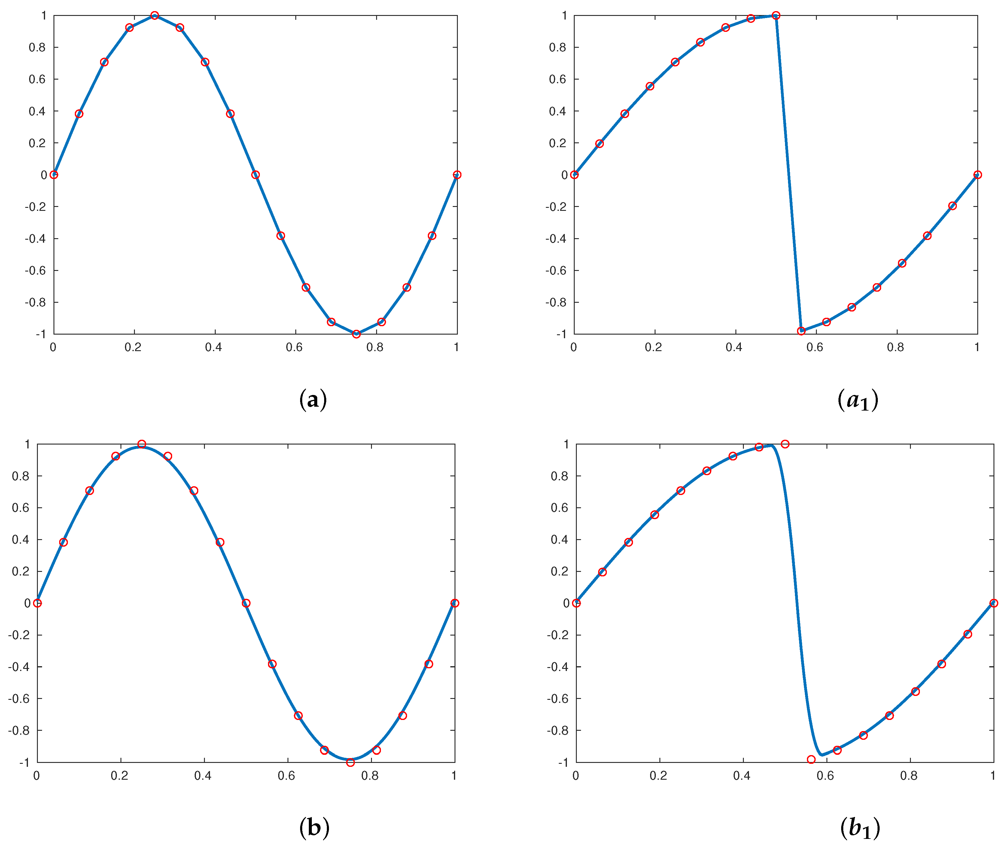
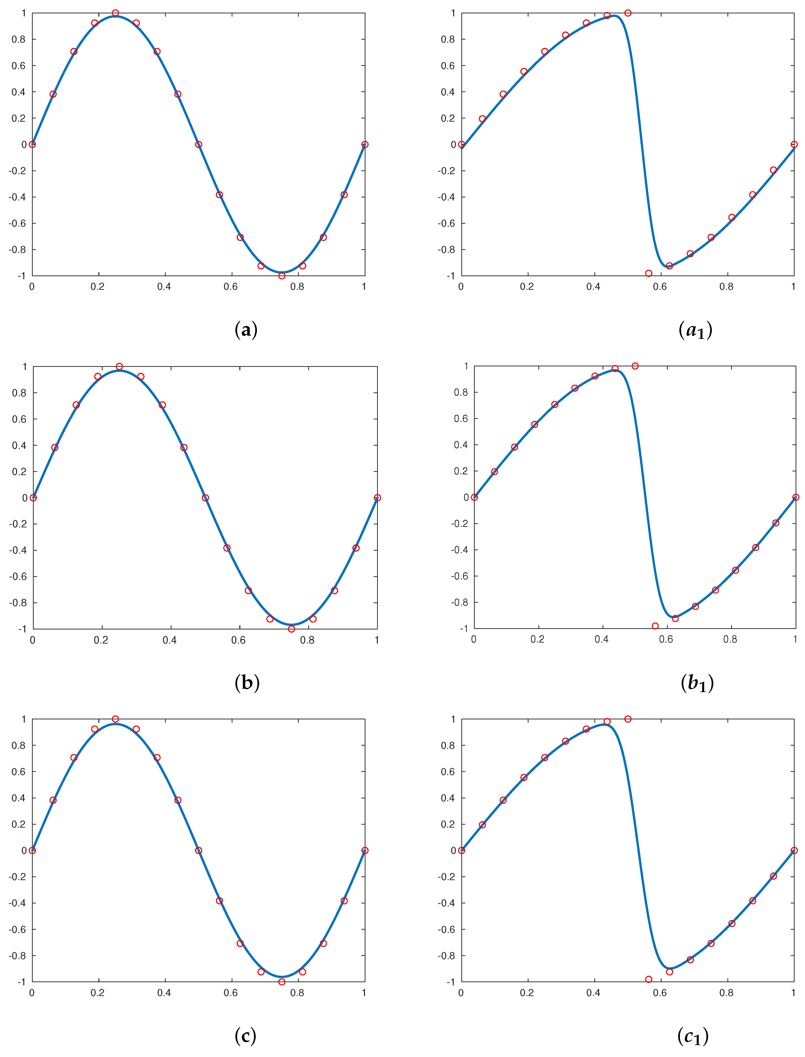
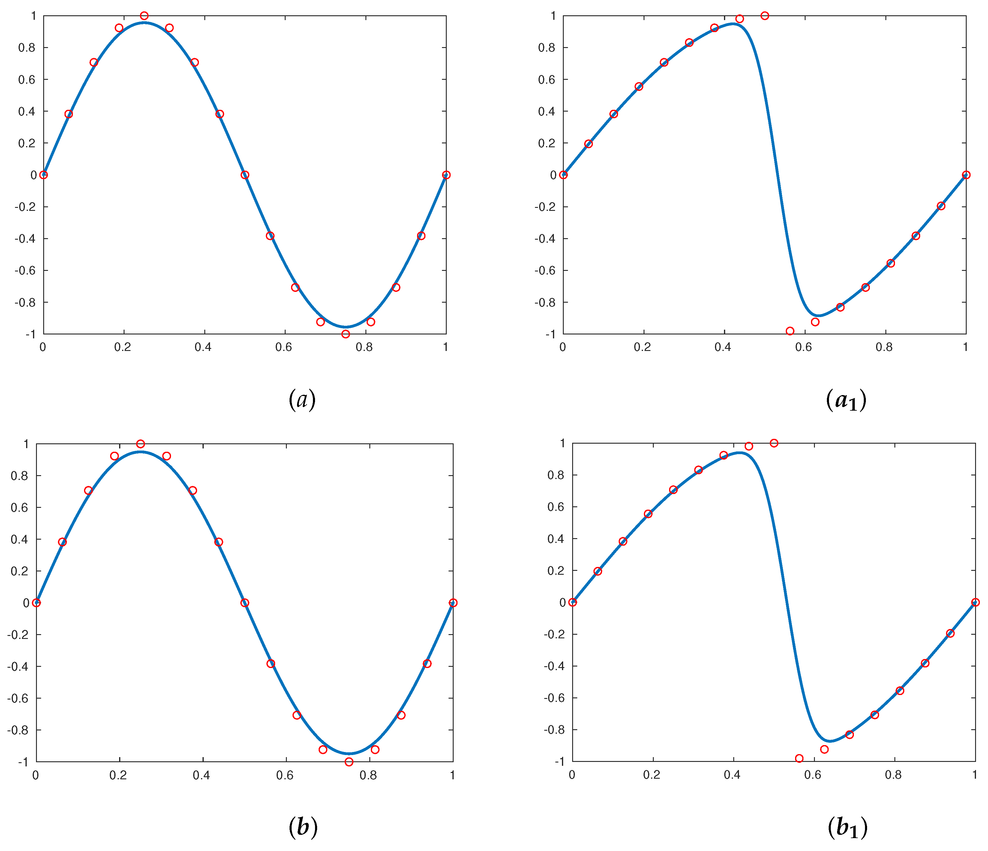
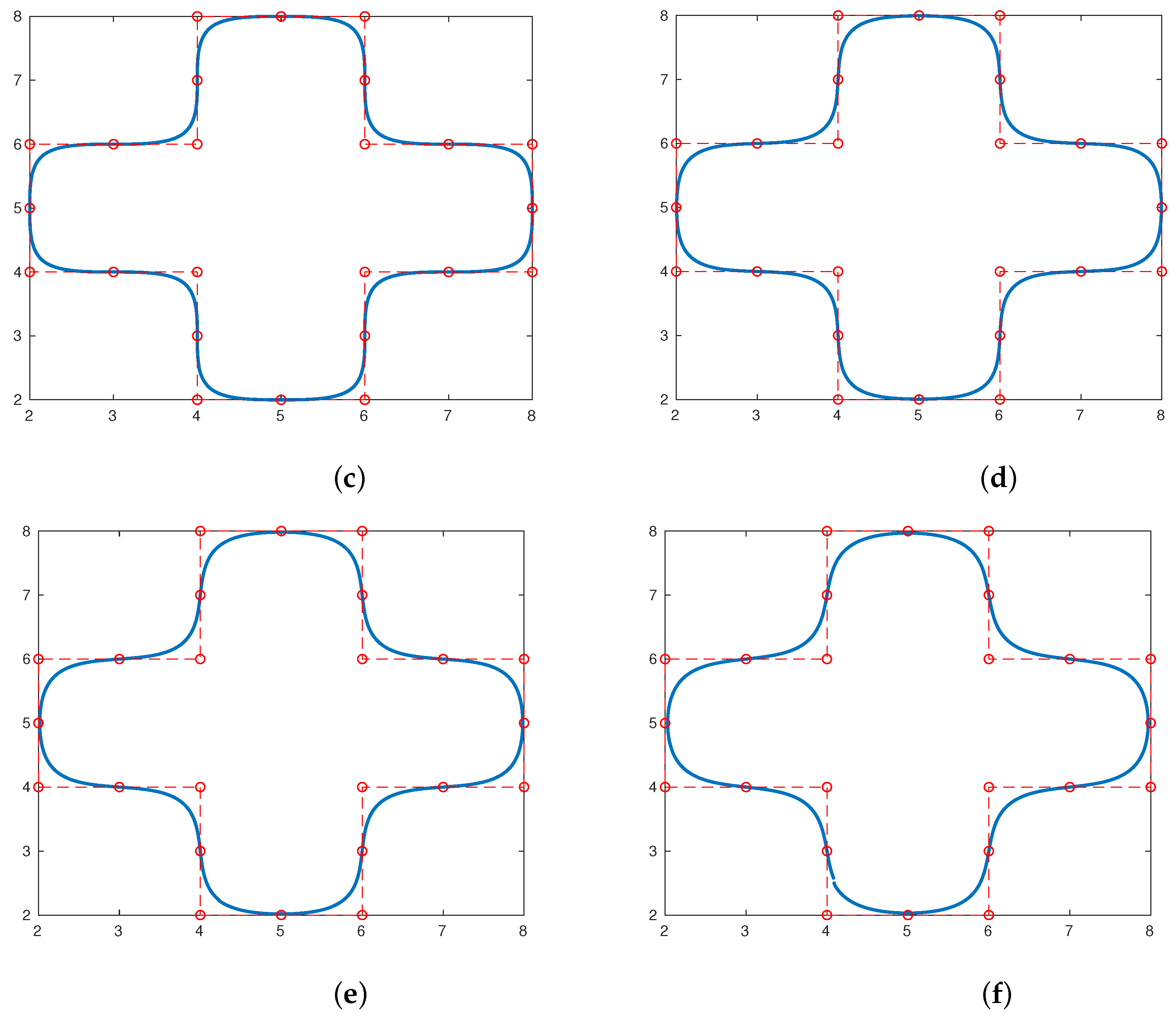
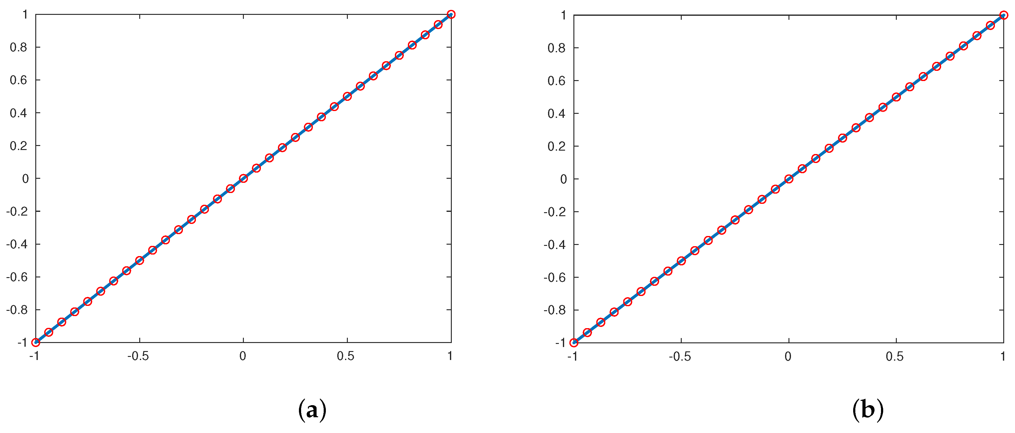
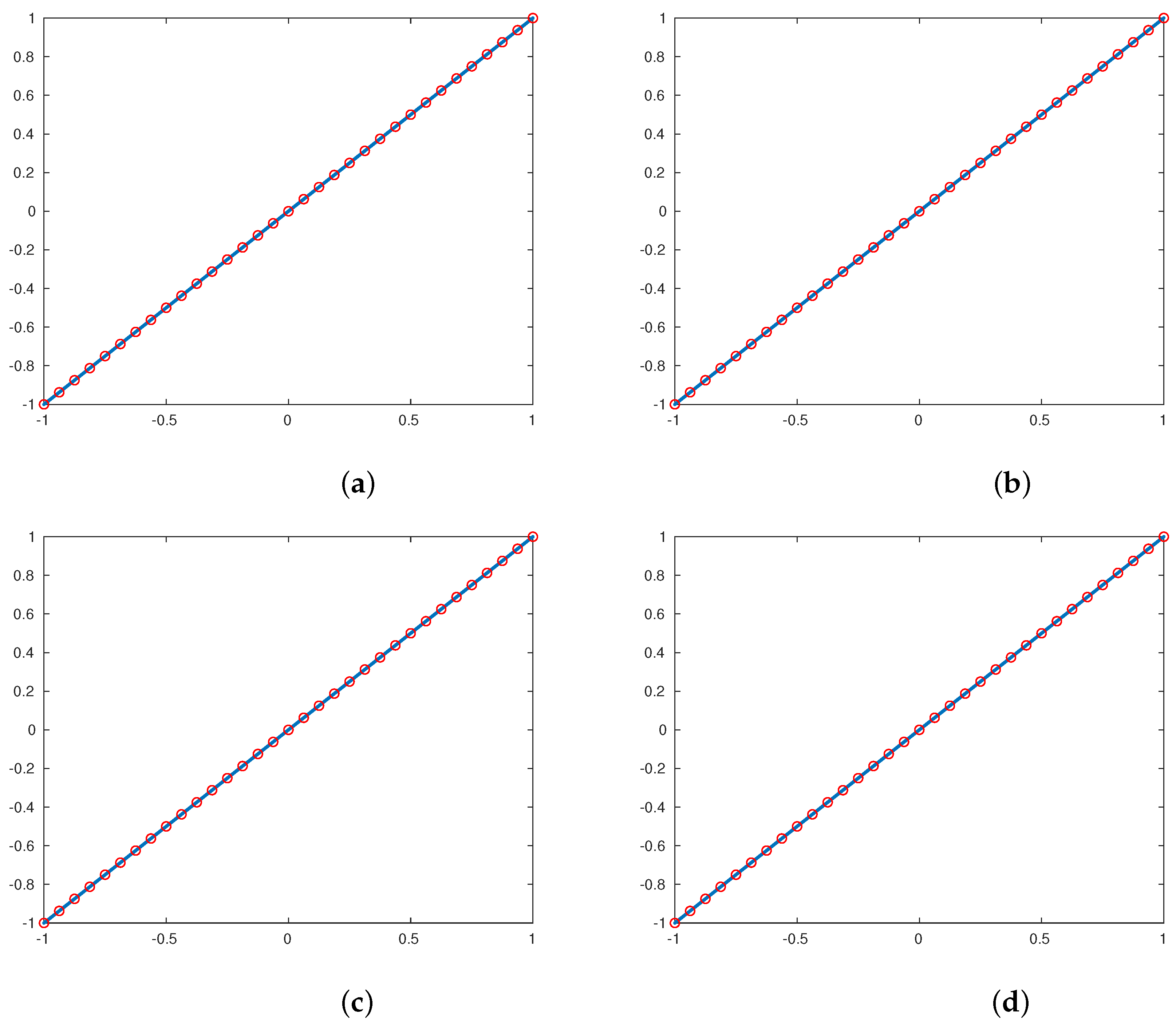
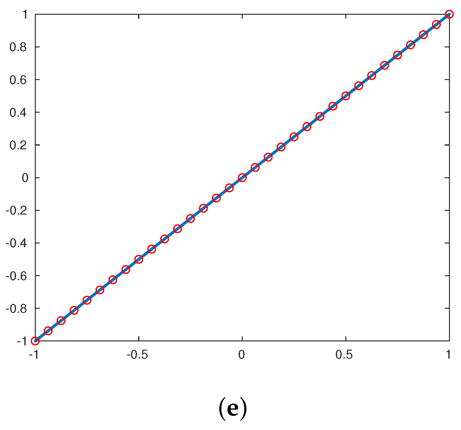
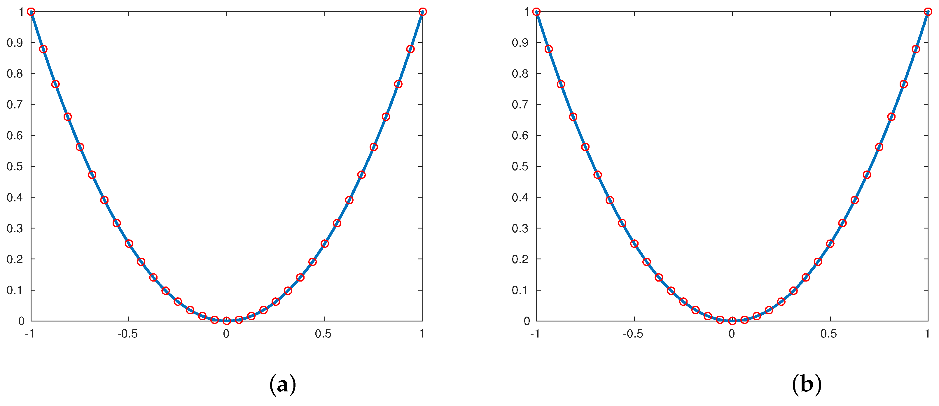
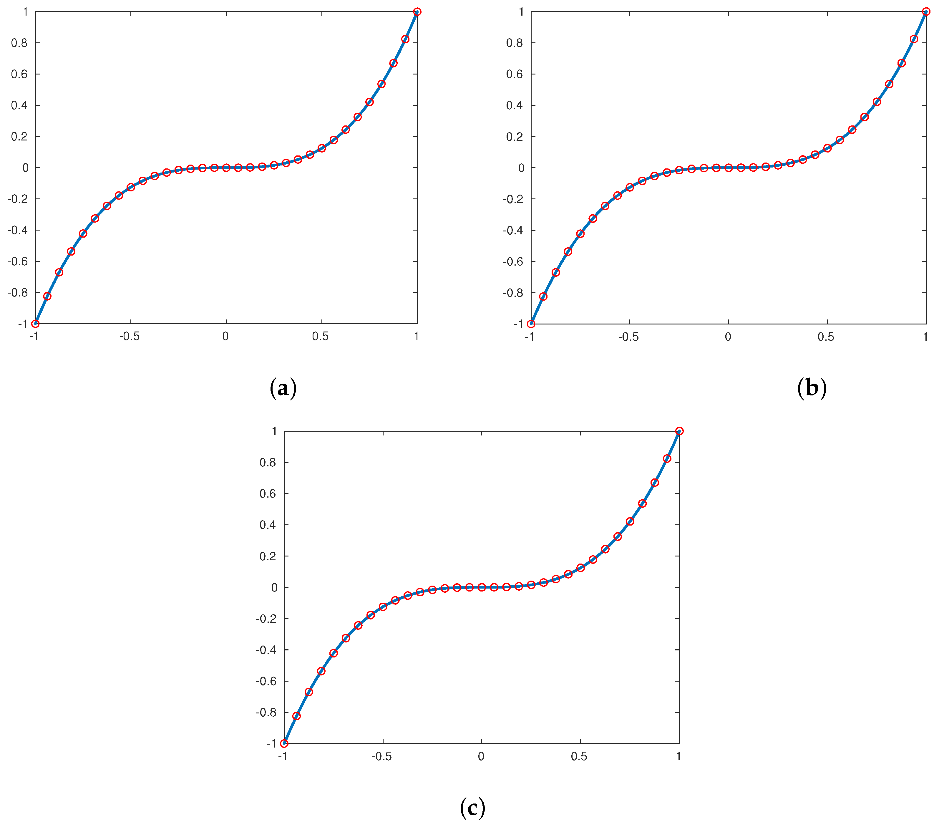
The generation degree of a subdivision scheme is the maximum degree of polynomials that can potentially be generated by the scheme, provided that the initial data are chosen correctly [13].

Theorem 16.

The families of subdivision schemes $S_{\alpha }$, for $\alpha =1,\dots ,6,$ defined in (8), (10), (11), (13), (15), (17), and (19), respectively, generate polynomials up to degree r, where

$$r=\left\{\begin{array}{cc}\alpha ,& \hfill ifw\ne \frac{1}{3},\\ \alpha +1,& \hfill ifw=\frac{1}{3}.\end{array}\right.$$

Proof. 

This proof is based on the same idea presented in [11].

If $w=\frac{1}{3}$, the family of Laurent polynomials (6) can be written as

$$a_{\alpha }\left(z\right)={\left(1+z+z^2\right)}^{(\alpha +1)+1}{b}_{\alpha }\left(z\right),$$

where

$$b_{\alpha }\left(z\right)={\displaystyle \frac{1}{3^{\alpha +1}{z}^m}}.$$

Since $b_{\alpha }\left(1\right)=\frac{1}{3^{\alpha +1}}$, then the families of subdivision schemes $S_{\alpha }$ generate polynomials up to the degree $\alpha +1$.

If $w\ne \frac{1}{3}$, the family of Laurent polynomials (6) can be written as

$$a_{\alpha }\left(z\right)={\left(1+z+z^2\right)}^{\alpha +1}{b}_{\alpha }\left(z\right),$$

where

$$b_{\alpha }\left(z\right)={\displaystyle \frac{w+(1-2w)z+w{z}^2}{3^{\alpha }{z}^m}}.$$

Since $b_{\alpha }\left(1\right)=\frac{1}{3^{\alpha }}$, then the families of subdivision schemes $S_{\alpha }$ generate polynomials up to degree $\alpha$. □

6. Gibbs Phenomenon

In this section, we are going to prove that the new family subdivision schemes do not suffer from the Gibbs phenomenon oscillations for some values of w.

Theorem 17.

The family subdivision schemes $S_{\alpha }$, for $\alpha =0,\dots ,6$ do not introduce the Gibbs phenomenon close to the discontinuities, for all $w\in ]0,1[,[0,\frac{3}{2}],[0,3[,[0,\frac{19}{6}],[0,\frac{51}{12}],[0,\frac{141}{30}]$, and $[0,\frac{393}{72}],$ respectively.

Proof. 

Using theorem 3.1 presented in [14], and the fact that the family subdivision schemes $S_{\alpha }$, for $\alpha =0,\dots ,6$, are convergent and have positives masks, for all $w\in ]0,1[,[0,\frac{3}{2}],[0,3[,[0,\frac{19}{6}],[0,\frac{51}{12}],[0,\frac{141}{30}]$, and $[0,\frac{393}{72}]$, respectively, we have the results. □

7. Comparison with Another Subdivision Schemes

In the following table, we present a comparison of our schemes with several schemes that we can find in the literature.

$\alpha$	n-point	Schemes	Type	Continuity	Coincide with
0	2-point	$S_0$ scheme	interpolatory	$C^0$ for $w\in ]0,1[$	Scheme [1] for $w=1/3$
1	3-point	$S_1$ scheme	approximating	$C^1$ for $w\in ]0,1[$
2	3-point	$S_2$ scheme	approximating	$C^2$ for $w\in ]0,1[$	Scheme [1] for $w=1/3$
					Scheme [3] for $w=1/8$
					Scheme [2] (with $\mu =1/18$) for $w=-1/2$
	3-point	Scheme in [2]	approximating	$C^1$
3	4-point	$S_3$ scheme	approximating	$C^3$ for $w\in ]0,1[$
	4-point	Scheme in [5]	approximating	$C^2$
	4-point	Scheme in [2]	approximating	$C^2$
	4-point	Scheme in [15]	approximating	$C^3$
4	5-point	$S_4$ scheme	approximating	$C^4$ for $w\in ]0,1[$	Scheme [7] (with $\mu =5/243$) for $w=-5/3$
					Scheme in [8] for $w=-81/a$
					(with $b=7a,c=6a\mathrm{and}d=3a$)
5	5-point	$S_5$ scheme	approximating	$C^5$ for $w\in ]0,1[$
	5-point	Scheme in [7]	approximating	$C^3$
	5-point	Scheme in [15]	approximating	$C^4$
6	6-point	$S_6$ scheme	approximating	$C^6$ for $w\in ]0,1[$
	6-point	Scheme in [15]	approximating	$C^5$

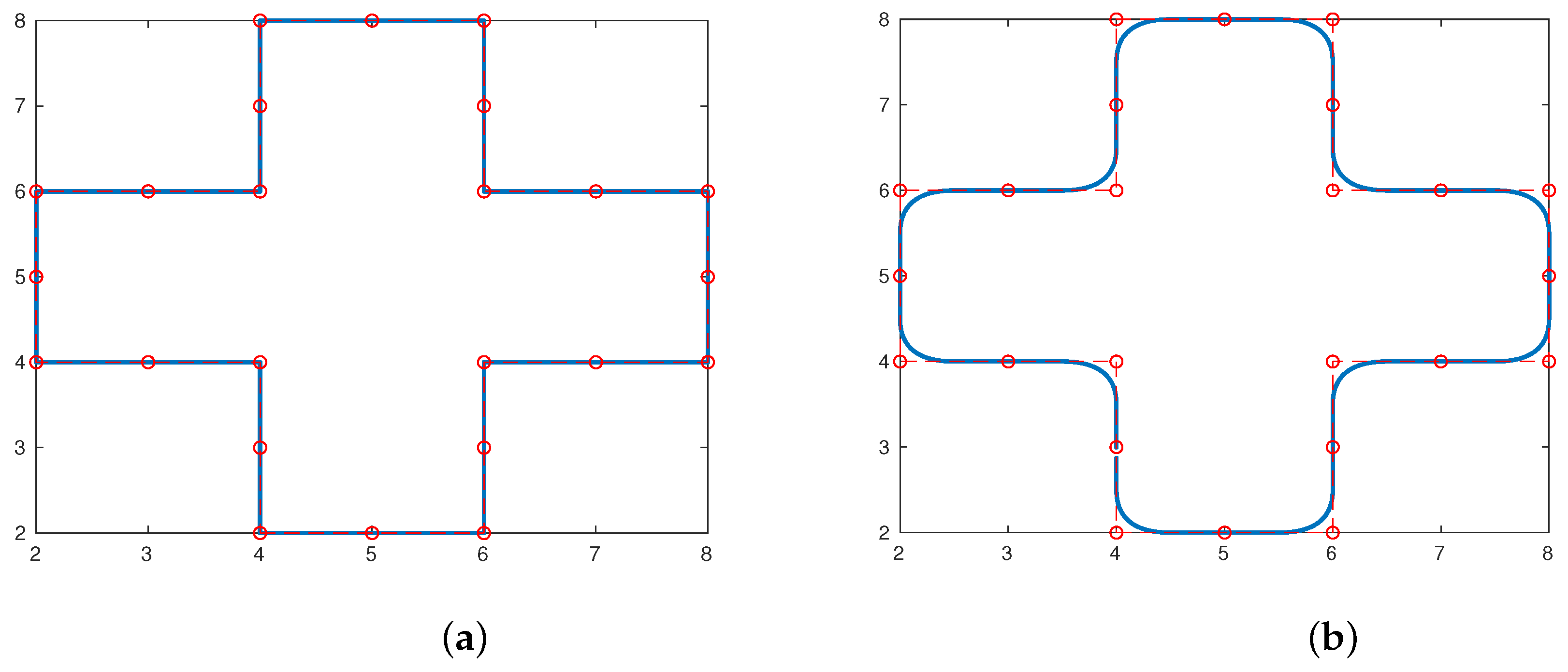
8. Numerical Tests

In this section, we present some numerical experiments in 1d and 2d.

Example 1.

 

In this example, we use two functions to obtain the initial data $f_n^0$, a continuous function defined by

$$f\left(x\right)=sin\left(\pi x\right),x\in [0,1]$$

(33)

and a discontinuous function defined by

$$g\left(x\right)=\left\{\begin{array}{c}sin\left(\pi x\right),x\in [0,0.5],\hfill \\ -sin\left(\pi x\right),x\in ]0.5,1].\hfill \end{array}\right.$$

(34)

For $w=\frac{1}{3}$, the limit functions obtained by the interpolatory subdivision scheme $S_0$, and the approximating subdivision schemes $S_{\alpha }$, $\alpha =1,\dots ,6$, using the continuous function given in (33) and the discontinuous function (34), have a $C^{\alpha }$ regularity, $\alpha =0,\dots ,6$, respectively, and they are displayed in Figure 1, Figure 2 and Figure 3. It is clear that (in the figures obtained by the discontinuous function (34)), all of these subdivision schemes do not produce the Gibbs oscillations close to the discontinuities in the limit functions.

Figure 1. Images on the left were obtained using the continuous function (33), images on the right were obtained using the discontinuous function (34) using five subdivision scales; the results shown in (a), (also ${\mathit{a}}_{\mathbf{1}}$) and (b), (also ${\mathit{b}}_{\mathbf{1}}$) were obtained by ${\mathit{S}}_{\mathbf{1}}$ (10) and ${\mathit{S}}_{\mathbf{2}}$ (11), respectively, where $\mathit{w}=\frac{\mathbf{1}}{\mathbf{3}}$. In this figure, the original sampling is represented in ∘.

Figure 2. Images on the left were obtained using the continuous function defined in (33), images on the right were obtained using the discontinuous function (34) using five subdivision scales; the results shown in (a), (also ${\mathit{a}}_{\mathbf{1}}$), (b), (also ${\mathit{b}}_{\mathbf{1}}$), and (c), (also ${\mathit{c}}_{\mathbf{1}}$) were obtained by ${\mathit{S}}_{\mathbf{2}}$ (11), ${\mathit{S}}_{\mathbf{3}}$ (13), and ${\mathit{S}}_{\mathbf{4}}$ (15), respectively, where $\mathit{w}=\frac{\mathbf{1}}{\mathbf{3}}$. In this figure, the original sampling is represented in ∘.

Figure 3. Images on the left were obtained using the continuous function defined in (33), images on the right were obtained using the discontinuous function (34), using five subdivision scales; the results shown in (a), (also ${\mathit{a}}_{\mathbf{1}}$) and (b), (also ${\mathit{b}}_{\mathbf{1}}$) were obtained by ${\mathit{S}}_{\mathbf{5}}$ (17) and ${\mathit{S}}_{\mathbf{6}}$ (19), respectively, where $\mathit{w}=\frac{\mathbf{1}}{\mathbf{3}}$. In this figure, the original sampling is represented in ∘.

Example 2.

For $w=\frac{1}{3}$, we will obtain, in this experiment, the limit functions for several curves in 2d, obtained by the interpolatory subdivision scheme $S_0$ and the approximating subdivision schemes $S_{\alpha }$, $\alpha =1,\dots ,6$, using the original data, are displayed in Figure 4 and Figure 5. Moreover, we can note that there are no Gibbs phenomena in the limit functions.

Figure 4. The limit functions in 2d using five subdivision scales; the results shown in (a–f) were obtained by $S_0$ (8), $S_1$ (10), $S_2$ (11), $S_3$ (13), $S_4$ (15) and $S_5$ (17), respectively, where $w=\frac{1}{3}$. In this figure, the original sampling is represented in ∘.

Figure 5. The limit function in 2d using five subdivision scales obtained by $S_6$ (19), where $w=\frac{1}{3}$. In this figure, the original sampling is represented in ∘.

Example 3.

In this experiment, we will test the reproduction polynomials property; here, we use the linear polynomial defined by $P_1\left(x\right)=x,\forall x\in [-1,1]$ to obtain the initials points. Applying the above subdivision schemes $S_{\alpha }$, $\alpha =0,\dots ,6$ with $w=\frac{1}{3}$, we obtain the same polynomial $P_1$ as a limit function of each subdivision scheme $S_{\alpha }$, the results are presented in Figure 6 and Figure 7.

Figure 6. The limit functions in 1d using five subdivision scales; the results shown in (a,b) were obtained by $S_0$ (8) and $S_1$ (10), respectively, where $w=\frac{1}{3}$. In this figure, the original sampling is represented in ∘.

Figure 7. The limit functions in 1d using five subdivision scales; the results shown in (a–e) were obtained by $S_2$ (11), $S_3$ (13), $S_4$ (15), $S_5$ (17), and $S_6$ (19), respectively, where $w=\frac{1}{3}$. In this figure, the original sampling is represented in ∘.

Example 4.

In Theorems 11 and 12, we proved that the subdivision schemes $S_2$ and $S_3$ reproduce the polynomials of degree 2 for $w=-1$ and $w=-\frac{4}{3}$, respectively; to check this, we used the polynomial defined by $P_2\left(x\right)=x^2,\forall x\in [-1,1]$ to obtain the initials points. Applying the subdivision schemes $S_2$, with $w=-1$ and $S_3$ with $w=-\frac{4}{3}$, we obtained the same polynomial $P_2$ as a limit function of both subdivision schemes $S_2$ and $S_3$. The results are presented in Figure 8.

Figure 8. The limit functions in 1d using five subdivision scales; the results shown in (a,b) were obtained by $S_2$ (11), where $w=-1$ and $S_3$ (13), where $w=-\frac{4}{3}$, respectively. In this figure, the original sampling is represented in ∘.

Example 5.

In this example, we will test the reproduction polynomials of degree 3 of the subdivision schemes $S_4$, $S_5$, and $S_6$. To obtain the initials points, we used the polynomial defined by $P_3\left(x\right)=x^3,\forall x\in [-1,1]$. Applying the subdivision schemes $S_4$, with $w=-\frac{5}{3}$, $S_5$ with $w=-2$ and $S_6$ with $w=-\frac{7}{3}$, we obtain the same polynomial $P_3$ as a limit function of each subdivision scheme $S_4$, $S_5$, and $S_6$. The results are presented in Figure 9.

Figure 9. The limit functions in 1d using five subdivision scales; the results shown in (a–c) were obtained by $S_4$ (15) with $w=-\frac{5}{3}$, $S_5$ (17) with $w=-2$ and $S_6$ (19) with $w=-\frac{7}{3}$, respectively. In this figure, the original sampling is represented in ∘.

9. Conclusions

In this paper, we presented and analyzed some new families of ternary subdivision schemes depending on free parameters. The families can be generalized to any order of approximation. We studied the convergence and the adaptation to the presence of discontinuities. We found some members in the families with very good properties. These subdivision schemes are good alternatives for the generation of curves and surfaces.

References

- Hassan, M.F.; Dodgson, N.A. Ternary and three point univariate subdivision schemes. In Curve and Surface Fitting: Saint-Malo 2002; Cohen, A., Merrien, J.-L., Schumaker, L.L., Eds.; Nashboro Press: Brentwood, UK, 2003; pp. 199–208. [Google Scholar]
- Rehan, K.; Siddiqi, S. A family of ternary subdivision schemes for curves. Appl. Math. Comput. 2015, 270, 114–123. [Google Scholar] [CrossRef]
- Siddiqi, S.S.; Rehan, K. A ternary three point scheme for curve designing. Int. J. Comput. Math. 2010, 87, 1709–1715. [Google Scholar] [CrossRef]
- Amat, S.; Choutri, A.; Ruiz, J.; Zouaoui, S. On a nonlinear 4-point ternary and non-interpolatory subdivision scheme eliminating the Gibbs phenomenon. Appl. Math. Comput. 2018, 320, 16–26. [Google Scholar] [CrossRef]
- Ko, K.P.; Lee, B.G.; Yoon, G.J. A ternary 4-point approximating subdivision scheme. Appl. Math. Comput. 2007, 190, 1563–1573. [Google Scholar] [CrossRef]
- Hassan, M.F.; Ivrissimitzis, I.P.; Dodgson, N.A.; Sabin, M.A. An interpolating 4-points C2 ternary stationary subdivision scheme. Comput. Aided Geom. Des. 2002, 19, 1–18. [Google Scholar] [CrossRef]
- Siddiqi, S.S.; Rehan, K. Ternary 2N-point Lagrange subdivision schemes. Appl. Math. Comput. 2014, 249, 444–452. [Google Scholar] [CrossRef]
- Zhang, L.; Ma, H.; Tang, S.; Tan, J. A combined approximating and interpolating ternary 4-point subdivision scheme. J. Comput. Appl. Math. 2019, 349, 63–578. [Google Scholar] [CrossRef]
- Rioul, O. Simple regularity criteria for subdivision schemes. SIAM J. Math. Anal. 1992, 23, 1544–1576. [Google Scholar] [CrossRef]
- Dyn, N.; Hormann, K. Polynomial reproduction by symmetric subdivision schemes. J. Approx. Theory 2008, 155, 28–42. [Google Scholar] [CrossRef] [Green Version]
- Conti, C.; Hormann, K. Polynomial reproduction for univariate subdivision schemes of any arity. J. Approx. Theory 2011, 163, 413–437. [Google Scholar] [CrossRef] [Green Version]
- Dyn, N. Interpolatory subdivision schemes. In Tutorials on Multiresolution in Geometric Modelling Summer School Lecture Notes Series Mathematics and Visualization; Iske, A., Quak, E., Floater, M., Eds.; Springer: Berlin, Germany, 2002; pp. 25–50. [Google Scholar]
- Romani, L. A Chaikin-based variant of Lane–Riesenfeld algorithm and its non-tensor product extension. Comput. Aided Geom. Des. 2015, 32, 22–49. [Google Scholar] [CrossRef]
- Zhou, J.; Zheng, H.; Zhang, B. Gibbs phenomenon for p-ary subdivision schemes. J. Inequal. Appl. 2019, 48. [Google Scholar] [CrossRef]
- Siddiqi, S.; Younis, M. Construction of ternary approximating subdivision schemes. UPB Sci. Bull. 2014, 76, 1223–7027. [Google Scholar]
Publisher’s Note: MDPI stays neutral with regard to jurisdictional claims in published maps and institutional affiliations. |
© 2022 by the authors. Licensee MDPI, Basel, Switzerland. This article is an open access article distributed under the terms and conditions of the Creative Commons Attribution (CC BY) license (https://creativecommons.org/licenses/by/4.0/).