


A Feature Selection Based on Improved Artificial Hummingbird Algorithm Using Random Opposition-Based Learning for Solving Waste Classification Problem


Abstract
1. Introduction
- In this study on solving the feature selection problem, the AHA is enhanced for the first time.
- An enhanced version of the AHA is proposed based on two operators: random opposition-based learning (ROBL) and opposition-based learning (OBL).
- The two proposed models are compared with the original algorithm and 12 different algorithms.
- The study applies the modified algorithms AHA-ROBL and AHA-OBL to the TrashNet database by using two pre-trained networks: VGG19 and ResNet.
- The two proposed algorithms each demonstrate a greater robustness and stability than other recent algorithms.
2. Literature Review
2.1. Waste Recycling Using Traditional Machine-Learning Algorithms
2.2. Waste Recycling Using Deep-Learning Algorithms
2.3. Waste Recycling Using Deep-Transfer Learning
3. Procedure and Methodology
- Data collection
- Data pre-processing
- Feature extraction techniques using pre-trained deep-learning models (VGG19 and Resnet20)
- Waste classification with the AHA-ROBL using AHA initialization followed by AHA scoring and AHA updating using an exploration mode and the AHA and an exploitation mode using ROBL
- Prediction and evaluation metrics
3.1. Dataset Description
3.2. Feature Extraction Using Pre-Trained CNN
3.2.1. VGG19
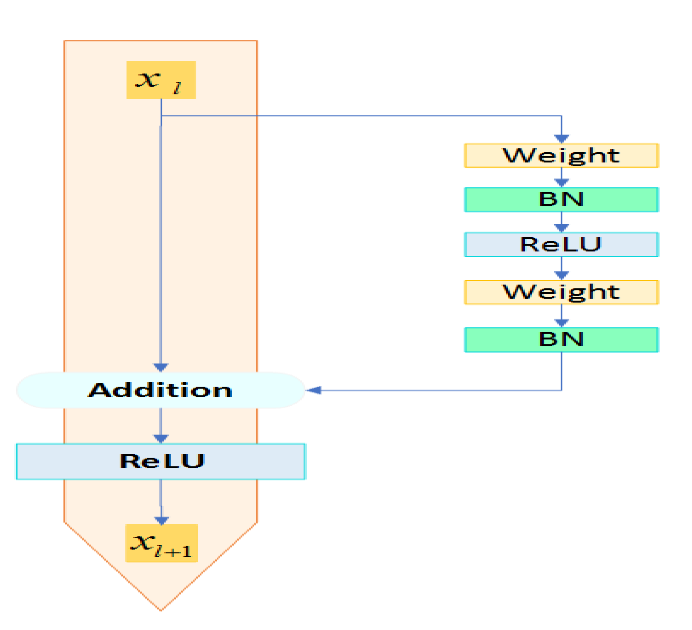
3.2.2. ResNet50
3.3. Artificial Hummingbird Algorithm (AHA)
| Algorithm 1 AHA pseudo-code. |
|
3.3.1. Guided Foraging
3.3.2. Territorial Foraging
3.3.3. Migration Foraging
3.4. Opposition-Based Learning (OBL)
3.5. Random Opposition-Based Learning (ROBL)
3.6. AHA-ROBL- and AHA-OBL-Based FS for Waste Classification
- 1.
- Pre-processing data
- 2.
- Deep feature extraction
- 3.
- Initialization
- 4.
- Score evaluation
- 5.
- Updating process
3.7. The Computational Complexity of the Two Proposed Algorithms (the AHA-OBL and AHA-ROBL)
3.7.1. Time Complexity
3.7.2. Space Complexity
4. Experimental Results
4.1. Parameter Settings for the Comparative Algorithms
4.2. Performance Metrics
- Mean accuracy : The metric is calculated as Equation (19):where M represents the number of runs, represents the number of samples in the test dataset, and and represent the classifier output label and the reference label class of sample r, respectively.
- Mean fitness value : The fitness value metric, which evaluates the performance of algorithms, is expressed as in Equation (20):where M is the number of runs and is the best fitness value for the run.
- Average recall : This indicates the percentage of predicted positive patterns that is defined as in Equation (21):The is calculated from the best object using Equation (22):
- Average precision : This indicates the frequency of true expected samples as in Equation (23):The mean precision () can be calculated by using Equation (24):
- Mean F-score : This metric is already in use for balanced data, which can be calculated using Equation (25):The mean F-score can be calculated using Equation (26):
- Mean features selection size : This indicates the average size of the selected attributes and is expressed as in Equation (27):
4.3. Results and Discussion
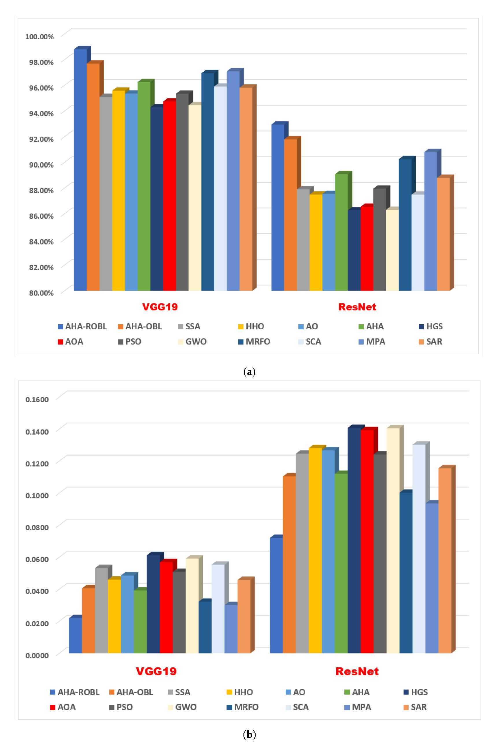
- Fitness: Table 2 displays the results of comparing the two proposed models (the AHA-ROBL and AHA-OBL) and competing algorithms. Based on the obtained results, it is evident that our AHA-ROBL model provides superior results, followed by the AHA-OBL. Two pre-trained CNN models (VGG19 and ResNet20) and the TrashNet dataset were chosen. The deep analysis of the dataset that was used revealed that the quantitative results obtained by using the proposed AHA-ROBL approach performed better with the two pre-trained CNN models (VGG19 and ResNet20) than the optimization algorithms, namely the basic AHA, HHO, SSA, AO, HGS, PSO, GWO, AOA, MRFO, SCA, MPA, and SAR. The results of the proposed VGG19 method are significantly superior to those of ResNet20. The AHA-OBL followed this with the lowest fitness value. The standard deviation was computed to evaluate the stability of the fitness value for each FS method. According to the standard deviation results, the traditional AHA-ROBL, AHA, and PSO approaches are more stable than other algorithms. HGS is the worst possible algorithm. It is important to note that the AHA-OBL obtained the second-best position using VGG19. In addition, for the ResNet20 deep features, the AHA-OBL was ranked second compared to the remaining 12 algorithms.
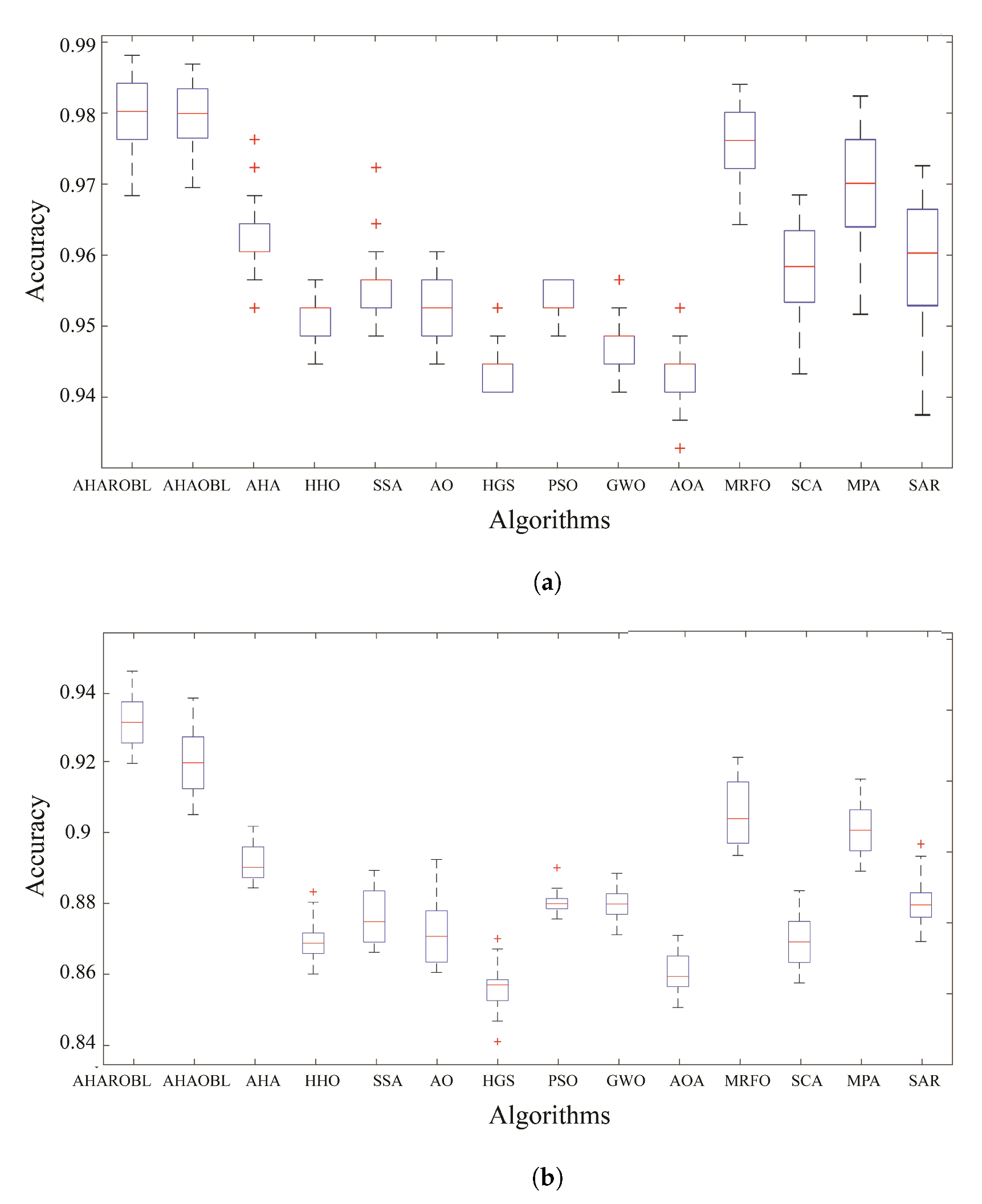
- Accuracy: The following observations can be drawn from the data presented in Table 3. First, the results demonstrated that the two proposed approaches (the AHA-ROBL and AHA-OBL) outperformed the optimization algorithms, namely the basic AHA, HHO, SSA, AO, HGS, PSO, GWO, AOA, MRFO, SCA, MPA, and SAR, in terms of quantitative results using the two pre-trained CNN models (VGG19 and ResNet20). The results of the proposed VGG19 method were significantly superior to those of ResNet. Compared to the 12 optimization algorithms, the MPA achieved the highest accuracy value.
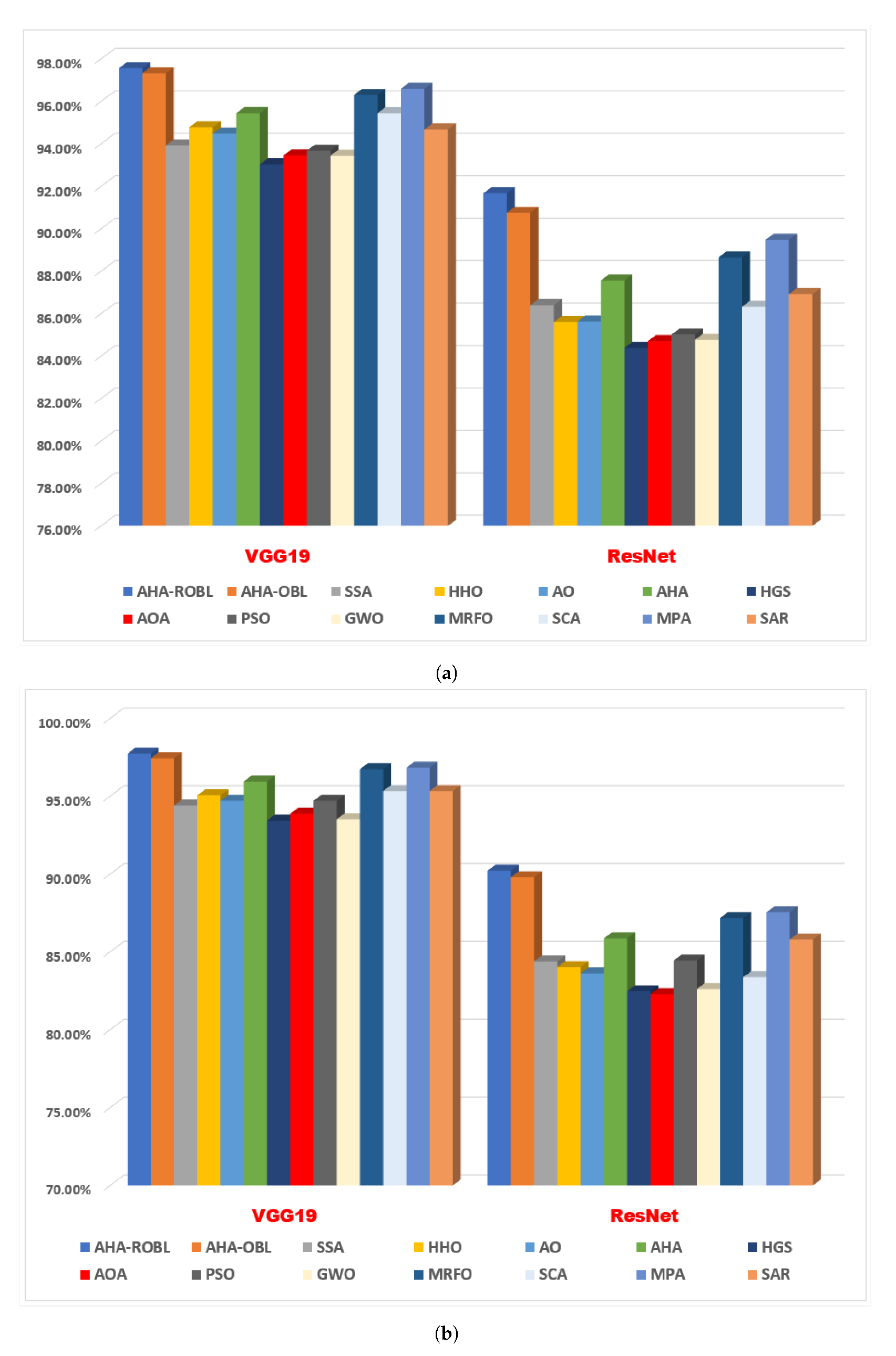
- Recall and precision: Table 4 and Table 5 list the recall and precision of the two proposed methods (the AHA-ROBL and AHA-OBL) with the 12 wrapper FS algorithms employing the two deep descriptors (VGG19 and ResNet20). By examining the average recall and precision values for the TrashNet dataset, it is evident that the AHA-ROBL outperformed all advanced competitor algorithms based on both deep features (VGG19 and ResNet20). Moreover, the average recall and precision obtained by using the AHA-ROBL based on VGG19 were superior to those obtained by the AHA-ROBL based on ResNet20. It can be seen that the AHA-ROBL based on deep descriptors has a strong stability for the TrashNet dataset due to the lower values of the standard deviation in terms of the precision and recall metrics. In addition, the AHA-OBL based on the deep VGG19 descriptor ranked in the second position in terms of average recall and precision for the TrashNet dataset. In addition, the MPA based on the deep VGG19 descriptor ranked in the third position in terms of average recall and precision for the TrashNet dataset. It can be seen that the AHA-ROBL based on the deep descriptors has a strong stability for the TrashNet dataset due to the lower values of the standard deviation in terms of the precision and recall metrics.
- Sensitivity and specificity: Table 6 and Table 7 list the sensitivity and specificity of the two proposed methods (the AHA-ROBL and AHA-OBL) with the 12 wrapper FS algorithms employing the two deep descriptors (VGG19 and ResNet20). By examining the average sensitivity and specificity values for the TrashNet dataset, it is evident that the AHA-ROBL outperformed all advanced competitor algorithms based on both deep features (VGG19 and ResNet20). Moreover, the average sensitivity and precision obtained by using the AHA-ROBL based on VGG19 are superior to those obtained by using the AHA-ROBL based on ResNet20. It can be seen that the AHA-ROBL based on the deep descriptors has a strong stability for the TrashNet dataset due to the lower values of the standard deviation in terms of the sensitivity and specificity metrics. In addition, the AHA-OBL based on the deep VGG19 descriptor ranked in the second position in terms of the average sensitivity and specificity for the TrashNet dataset. Moreover, the AHA based on the deep VGG19 descriptor ranked in the second position in terms of the average sensitivity and specificity for the TrashNet dataset. It can be seen that the AHA-ROBL based on the deep descriptors has a strong stability for the TrashNet dataset due to the lower values of the standard deviation in terms of the sensitivity and specificity metrics.
- F-score: In terms of the F-score, Table 8 reveals that the two proposed methods (the AHA-ROBL and AHA-OBL) were based on the pre-trained CNNs (VGG19 and ResNet20) and outperformed all the other competitors. In addition, fierce competition existed between the MPAs based on ResNet20 and VGG19 for the third position. Moreover, the GWO based on the deep features achieved lower F-score values.
- Selection ratio: According to the results of Table 9, which depict the mean rate of the selection ratio and its standard deviation, the AHA-ROBL exhibited excellent performance in selecting relevant deep features from the TrashNet dataset. In addition, we can observe that the proposed AHA-ROBL method provided an excellent behavior for selecting the optimal set of relevant deep features. The deep analysis of the dataset that was used revealed that the quantitative results obtained by using the proposed AHA-ROBL approach performed better with the two pre-trained CNN models (VGG19 and ResNet20) than the optimization algorithms, namely the basic AHA, HHO, SSA, AO, HGS, PSO, GWO, and AOA. Clearly, the proposed VGG19 approach produces significantly superior results to ResNet20. It is important to mention that the second-best place was obtained by the AHA using VGG19.
- Average execution time: Table 10 reveals that the two proposed methods (the AHA-ROBL and AHA-OBL) based on the pre-trained CNNs (VGG19 and ResNet20) outperformed 75% of the other competitors. In addition, the AHA outperformed most of the other competitors.
4.4. The Wilcoxon Test
4.5. Graphical Analysis
5. Comparative Study with the Existing Works
6. Conclusions and Future Work
Author Contributions
Funding
Institutional Review Board Statement
Informed Consent Statement
Data Availability Statement
Conflicts of Interest
References
- Geyer, R.; Jambeck, J.; Law, K. Producción, uso y destino de todos los plásticos jamás fabricados. Sci. Adv. 2017, 3, 1207–1221. [Google Scholar]
- Kumar, S.; Smith, S.; Fowler, G.; Velis, C.; Rena; Kumar, R.; Cheeseman, C. Challenges and opportunities associated with waste management in India. R. Soc. Open Sci. 2017, 4, 160764. [Google Scholar] [CrossRef] [PubMed]
- Bircanoğlu, C.; Atay, M.; Beşer, F.; Genç, Ö.; Kızrak, M.A. RecycleNet: Intelligent waste sorting using deep neural networks. In Proceedings of the 2018 Innovations in Intelligent Systems and Applications (INISTA), Thessaloniki, Greece, 3–5 July 2018; pp. 1–7. [Google Scholar]
- Borowski, P.F. Environmental pollution as a threats to the ecology and development in Guinea Conakry. Environ. Prot. Nat. Resour. Środowiska I Zasobów Nat. 2017, 28, 27–32. [Google Scholar] [CrossRef]
- Zelazinski, T.; Ekielski, A.; Tulska, E.; Vladut, V.; Durczak, K. Wood dust application for improvment of selected properties of thermoplastic starch. Inmateh. Agric. Eng 2019, 58, 37–44. [Google Scholar]
- Tiyajamorn, P.; Lorprasertkul, P.; Assabumrungrat, R.; Poomarin, W.; Chancharoen, R. Automatic Trash Classification using Convolutional Neural Network Machine Learning. In Proceedings of the 2019 IEEE International Conference on Cybernetics and Intelligent Systems (CIS) and IEEE Conference on Robotics, Automation and Mechatronics (RAM), Bangkok, Thailand, 18–20 November 2019; pp. 71–76. [Google Scholar]
- Yu, Y. A Computer Vision Based Detection System for Trash Bins Identification during Trash Classification. In Proceedings of the Journal of Physics: Conference Series, 2nd International Conference on Electronic Engineering and Informatics, Lanzhou, China, 17–19 July 2020; IOP Publishing: Bristol, UK, 2020; Volume 1617, p. 012015. [Google Scholar]
- Ruiz, V.; Sánchez, Á.; Vélez, J.F.; Raducanu, B. Automatic image-based waste classification. In Proceedings of the International Work-Conference on the Interplay Between Natural and Artificial Computation, Almería, Spain, 3–7 June 2019; Springer: Berlin/Heidelberg, Germany, 2019; pp. 422–431. [Google Scholar]
- Singh, A.; Rai, N.; Sharma, P.; Nagrath, P.; Jain, R. Age, Gender Prediction and Emotion recognition using Convolutional Neural Network. In Proceedings of the International Conference on Innovative Computing & Communication (ICICC), New Delhi, India, 20–21 February 2021. [Google Scholar]
- Mohmmadzadeh, H.; Gharehchopogh, F.S. An efficient binary chaotic symbiotic organisms search algorithm approaches for feature selection problems. J. Supercomput. 2021, 77, 9102–9144. [Google Scholar] [CrossRef]
- Naseri, T.S.; Gharehchopogh, F.S. A Feature Selection Based on the Farmland Fertility Algorithm for Improved Intrusion Detection Systems. J. Netw. Syst. Manag. 2022, 30, 1–27. [Google Scholar] [CrossRef]
- Abd Elminaam, D.S.; Nabil, A.; Ibraheem, S.A.; Houssein, E.H. An efficient marine predators algorithm for feature selection. IEEE Access 2021, 9, 60136–60153. [Google Scholar] [CrossRef]
- Faramarzi, A.; Heidarinejad, M.; Stephens, B.; Mirjalili, S. Equilibrium optimizer: A novel optimization algorithm. Knowl.-Based Syst. 2020, 191, 105190. [Google Scholar] [CrossRef]
- Elgamal, Z.M.; Yasin, N.M.; Sabri, A.Q.M.; Sihwail, R.; Tubishat, M.; Jarrah, H. Improved equilibrium optimization algorithm using elite opposition-based learning and new local search strategy for feature selection in medical datasets. Computation 2021, 9, 68. [Google Scholar] [CrossRef]
- AbdElminaam, D.S.; Neggaz, N.; Gomaa, I.A.E.; Ismail, F.H.; Elsawy, A. AOM-MPA: Arabic Opinion Mining using Marine Predators Algorithm based Feature Selection. In Proceedings of the 2021 International Mobile, Intelligent and Ubiquitous Computing Conference (MIUCC), Cairo, Egypt, 26—27 May 2021; pp. 395–402. [Google Scholar]
- Abd Elminaam, D.S.; Neggaz, N.; Ahmed, I.A.; Abouelyazed, A.E.S. Swarming behavior of Harris hawks optimizer for Arabic opinion mining. Comput. Mater. Contin. 2021, 69, 4129–4149. [Google Scholar] [CrossRef]
- Shaban, H.; Houssein, E.H.; Pérez-Cisneros, M.; Oliva, D.; Hassan, A.Y.; Ismaeel, A.A.; AbdElminaam, D.S.; Deb, S.; Said, M. Identification of Parameters in Photovoltaic Models through a Runge Kutta Optimizer. Mathematics 2021, 9, 2313. [Google Scholar] [CrossRef]
- Abdelminaam, D.S.; Said, M.; Houssein, E.H. Turbulent flow of water-based optimization using new objective function for parameter extraction of six photovoltaic models. IEEE Access 2021, 9, 35382–35398. [Google Scholar] [CrossRef]
- Deb, S.; Abdelminaam, D.S.; Said, M.; Houssein, E.H. Recent Methodology-Based Gradient-Based Optimizer for Economic Load Dispatch Problem. IEEE Access 2021, 9, 44322–44338. [Google Scholar] [CrossRef]
- Deb, S.; Houssein, E.H.; Said, M.; AbdElminaam, D.S. Performance of Turbulent Flow of Water Optimization on Economic Load Dispatch Problem. IEEE Access 2021, 9, 77882–77893. [Google Scholar] [CrossRef]
- El-Ashmawi, W.H.; Abd Elminaam, D.S. A modified squirrel search algorithm based on improved best fit heuristic and operator strategy for bin packing problem. Appl. Soft Comput. 2019, 82, 105565. [Google Scholar] [CrossRef]
- Abdul-Minaam, D.S.; Al-Mutairi, W.M.E.S.; Awad, M.A.; El-Ashmawi, W.H. An adaptive fitness-dependent optimizer for the one-dimensional bin packing problem. IEEE Access 2020, 8, 97959–97974. [Google Scholar] [CrossRef]
- Dizaji, Z.A.; Gharehchopogh, F.S. A hybrid of ant colony optimization and chaos optimization algorithms approach for software cost estimation. Indian J. Sci. Technol. 2015, 8, 128. [Google Scholar] [CrossRef]
- Gharehchopogh, F.S.; Abdollahzadeh, B. An efficient harris hawk optimization algorithm for solving the travelling salesman problem. Clust. Comput. 2022, 25, 1981–2005. [Google Scholar] [CrossRef]
- Gharehchopogh, F.S.; Farnad, B.; Alizadeh, A. A modified farmland fertility algorithm for solving constrained engineering problems. Concurr. Comput. Pract. Exp. 2021, 33, e6310. [Google Scholar] [CrossRef]
- Zaman, H.R.R.; Gharehchopogh, F.S. An improved particle swarm optimization with backtracking search optimization algorithm for solving continuous optimization problems. Eng. Comput. 2021, 2021, 1–35. [Google Scholar] [CrossRef]
- Goldanloo, M.J.; Gharehchopogh, F.S. A hybrid OBL-based firefly algorithm with symbiotic organisms search algorithm for solving continuous optimization problems. J. Supercomput. 2022, 78, 3998–4031. [Google Scholar] [CrossRef]
- Lan, P.; Xia, K.; Pan, Y.; Fan, S. An improved equilibrium optimizer algorithm and its application in LSTM neural network. Symmetry 2021, 13, 1706. [Google Scholar] [CrossRef]
- Ma, H.; Simon, D.; Siarry, P.; Yang, Z.; Fei, M. Biogeography-based optimization: A 10-year review. IEEE Trans. Emerg. Top. Comput. Intell. 2017, 1, 391–407. [Google Scholar] [CrossRef]
- Niccolai, A.; Bettini, L.; Zich, R. Optimization of electric vehicles charging station deployment by means of evolutionary algorithms. Int. J. Intell. Syst. 2021, 36, 5359–5383. [Google Scholar] [CrossRef]
- Das, S.; Mullick, S.S.; Suganthan, P.N. Recent advances in differential evolution–an updated survey. Swarm Evol. Comput. 2016, 27, 1–30. [Google Scholar] [CrossRef]
- Saidala, R.K.; Devarakonda, N. Multi-swarm whale optimization algorithm for data clustering problems using multiple cooperative strategies. Int. J. Intell. Syst. Appl. 2018, 11, 36. [Google Scholar] [CrossRef]
- Mirjalili, S. Genetic algorithm. In Evolutionary Algorithms and Neural Networks; Springer: Berlin/Heidelberg, Germany, 2019; pp. 43–55. [Google Scholar]
- Elsisi, M. Optimal design of nonlinear model predictive controller based on new modified multitracker optimization algorithm. Int. J. Intell. Syst. 2020, 35, 1857–1878. [Google Scholar] [CrossRef]
- Massobrio, R.; Toutouh, J.; Nesmachnow, S.; Alba, E. Infrastructure deployment in vehicular communication networks using a parallel multiobjective evolutionary algorithm. Int. J. Intell. Syst. 2017, 32, 801–829. [Google Scholar] [CrossRef]
- Simon, D. Evolutionary Optimization Algorithms; John Wiley & Sons: Hoboken, NJ, USA, 2013. [Google Scholar]
- Garg, H. Multi-objective optimization problem of system reliability under intuitionistic fuzzy set environment using Cuckoo Search algorithm. J. Intell. Fuzzy Syst. 2015, 29, 1653–1669. [Google Scholar] [CrossRef]
- Bolaji, A.L.; Al-Betar, M.A.; Awadallah, M.A.; Khader, A.T.; Abualigah, L.M. A comprehensive review: Krill Herd algorithm (KH) and its applications. Appl. Soft Comput. 2016, 49, 437–446. [Google Scholar] [CrossRef]
- Garg, H. A hybrid PSO-GA algorithm for constrained optimization problems. Appl. Math. Comput. 2016, 274, 292–305. [Google Scholar] [CrossRef]
- Eusuff, M.M.; Lansey, K.E. Water distribution network design using the shuffled frog leaping algorithm. In Proceedings of the Bridging the Gap: Meeting the World’s Water and Environmental Resources Challenges, Orlando, FL, USA, 20–24 May 2001; pp. 1–8. [Google Scholar]
- Ma, H.; Ye, S.; Simon, D.; Fei, M. Conceptual and numerical comparisons of swarm intelligence optimization algorithms. Soft Comput. 2017, 21, 3081–3100. [Google Scholar] [CrossRef]
- Garg, V.; Deep, K. Performance of Laplacian Biogeography-Based Optimization Algorithm on CEC 2014 continuous optimization benchmarks and camera calibration problem. Swarm Evol. Comput. 2016, 27, 132–144. [Google Scholar] [CrossRef]
- Yang, G.P.; Liu, S.Y.; Zhang, J.K.; Feng, Q.X. Control and synchronization of chaotic systems by an improved biogeography-based optimization algorithm. Appl. Intell. 2013, 39, 132–143. [Google Scholar] [CrossRef]
- García-Torres, J.M.; Damas, S.; Cordón, O.; Santamaría, J. A case study of innovative population-based algorithms in 3D modeling: Artificial bee colony, biogeography-based optimization, harmony search. Expert Syst. Appl. 2014, 41, 1750–1762. [Google Scholar] [CrossRef]
- Ma, H. An analysis of the equilibrium of migration models for biogeography-based optimization. Inf. Sci. 2010, 180, 3444–3464. [Google Scholar] [CrossRef]
- Ma, H.; Ni, S.; Sun, M. Equilibrium species counts and migration model tradeoffs for biogeography-based optimization. In Proceedings of the 48h IEEE Conference on Decision and Control (CDC) Held Jointly with 2009 28th Chinese Control Conference, Shanghai, China, 15–18 December 2009; pp. 3306–3310. [Google Scholar]
- Ma, H.; Fei, M.; Ding, Z.; Jin, J. Biogeography-based optimization with ensemble of migration models for global numerical optimization. In Proceedings of the 2012 IEEE Congress on Evolutionary Computation, Brisbane, Australia, 10–15 June 2012; pp. 1–8. [Google Scholar]
- Gong, W.; Cai, Z.; Ling, C.X.; Li, H. A real-coded biogeography-based optimization with mutation. Appl. Math. Comput. 2010, 216, 2749–2758. [Google Scholar] [CrossRef]
- Niu, Q.; Zhang, L.; Li, K. A biogeography-based optimization algorithm with mutation strategies for model parameter estimation of solar and fuel cells. Energy Convers. Manag. 2014, 86, 1173–1185. [Google Scholar] [CrossRef]
- Roy, P.; Mandal, D. Quasi-oppositional biogeography-based optimization for multi-objective optimal power flow. Electr. Power Components Syst. 2011, 40, 236–256. [Google Scholar] [CrossRef]
- Kim, S.S.; Byeon, J.H.; Lee, S.; Liu, H. A grouping biogeography-based optimization for location area planning. Neural Comput. Appl. 2015, 26, 2001–2012. [Google Scholar] [CrossRef]
- Feng, Q.; Liu, S.; Wu, Q.; Tang, G.; Zhang, H.; Chen, H. Modified biogeography-based optimization with local search mechanism. J. Appl. Math. 2013, 2013, 960524. [Google Scholar] [CrossRef]
- Lim, W.L.; Wibowo, A.; Desa, M.I.; Haron, H. A biogeography-based optimization algorithm hybridized with tabu search for the quadratic assignment problem. Comput. Intell. Neurosci. 2016, 2016, 27. [Google Scholar] [CrossRef]
- Yang, Y. A modified biogeography-based optimization for the flexible job shop scheduling problem. Math. Probl. Eng. 2015, 2015, 184643. [Google Scholar] [CrossRef]
- Li, X.; Yin, M. Hybrid differential evolution with biogeography-based optimization for design of a reconfigurable antenna array with discrete phase shifters. Int. J. Antennas Propag. 2011, 2011, 685629. [Google Scholar] [CrossRef]
- Sinha, S.; Bhola, A.; Panchal, V.; Singhal, S.; Abraham, A. Resolving mixed pixels by hybridization of biogeography based optimization and ant colony optimization. In Proceedings of the 2012 IEEE Congress on Evolutionary Computation, Brisbane, Australia, 10–15 June 2012; pp. 1–6. [Google Scholar]
- Wang, G.G.; Gandomi, A.H.; Alavi, A.H. An effective krill herd algorithm with migration operator in biogeography-based optimization. Appl. Math. Model. 2014, 38, 2454–2462. [Google Scholar] [CrossRef]
- Heidari, A.A.; Abbaspour, R.A.; Jordehi, A.R. An efficient chaotic water cycle algorithm for optimization tasks. Neural Comput. Appl. 2017, 28, 57–85. [Google Scholar] [CrossRef]
- Krithiga, R.; Ilavarasan, E. A Novel Hybrid Algorithm to Classify Spam Profiles in Twitter. Webology 2020, 17, 260–279. [Google Scholar]
- Sawhney, R.; Mathur, P.; Shankar, R. A firefly algorithm based wrapper-penalty feature selection method for cancer diagnosis. In Proceedings of the International Conference on Computational Science and Its Applications, Melbourne, Australia, 2–5 July 2018; Springer: Berlin/Heidelberg, Germany, 2018; pp. 438–449. [Google Scholar]
- Mirjalili, S.; Gandomi, A.H.; Mirjalili, S.Z.; Saremi, S.; Faris, H.; Mirjalili, S.M. Salp Swarm Algorithm: A bio-inspired optimizer for engineering design problems. Adv. Eng. Softw. 2017, 114, 163–191. [Google Scholar] [CrossRef]
- Faris, H.; Mafarja, M.M.; Heidari, A.A.; Aljarah, I.; Ala’M, A.Z.; Mirjalili, S.; Fujita, H. An efficient binary salp swarm algorithm with crossover scheme for feature selection problems. Knowl.-Based Syst. 2018, 154, 43–67. [Google Scholar] [CrossRef]
- Sayed, G.I.; Khoriba, G.; Haggag, M.H. A novel chaotic salp swarm algorithm for global optimization and feature selection. Appl. Intell. 2018, 48, 3462–3481. [Google Scholar] [CrossRef]
- Harifi, S.; Khalilian, M.; Mohammadzadeh, J.; Ebrahimnejad, S. Emperor Penguins Colony: A new metaheuristic algorithm for optimization. Evol. Intell. 2019, 12, 211–226. [Google Scholar] [CrossRef]
- Zheng, T.; Luo, W. An improved squirrel search algorithm for optimization. Complexity 2019, 2019, 6291968. [Google Scholar] [CrossRef]
- Wang, Y.; Du, T. An improved squirrel search algorithm for global function optimization. Algorithms 2019, 12, 80. [Google Scholar] [CrossRef]
- Li, S.; Chen, H.; Wang, M.; Heidari, A.A.; Mirjalili, S. Slime mould algorithm: A new method for stochastic optimization. Future Gener. Comput. Syst. 2020, 111, 300–323. [Google Scholar] [CrossRef]
- Faramarzi, A.; Heidarinejad, M.; Mirjalili, S.; Gandomi, A.H. Marine predators algorithm: A nature-inspired Metaheuristic. Expert Syst. Appl. 2020, 152, 113377. [Google Scholar] [CrossRef]
- Houssein, E.H.; Abdelminaam, D.S.; Hassan, H.N.; Al-Sayed, M.M.; Nabil, E. A Hybrid Barnacles Mating Optimizer Algorithm With Support Vector Machines for Gene Selection of Microarray Cancer Classification. IEEE Access 2021, 9, 64895–64905. [Google Scholar] [CrossRef]
- Zhao, W.; Wang, L.; Mirjalili, S. Artificial hummingbird algorithm: A new bio-inspired optimizer with its engineering applications. Comput. Methods Appl. Mech. Eng. 2022, 388, 114194. [Google Scholar] [CrossRef]
- Halim, A.H.; Ismail, I.; Das, S. Performance assessment of the metaheuristic optimization algorithms: An exhaustive review. Artif. Intell. Rev. 2021, 54, 2323–2409. [Google Scholar] [CrossRef]
- Liu, M.; Li, Y.; Huo, Q.; Li, A.; Zhu, M.; Qu, N.; Chen, L.; Xia, M. A two-way parallel slime mold algorithm by flow and distance for the travelling salesman problem. Appl. Sci. 2020, 10, 6180. [Google Scholar] [CrossRef]
- Premkumar, M.; Jangir, P.; Sowmya, R.; Alhelou, H.H.; Heidari, A.A.; Chen, H. MOSMA: Multi-objective slime mould algorithm based on elitist non-dominated sorting. IEEE Access 2020, 9, 3229–3248. [Google Scholar] [CrossRef]
- İzci, D.; Ekinci, S.; Ekinci, S. Comparative performance analysis of slime mould algorithm for efficient design of proportional–integral–derivative controller. Electrica 2021, 21, 151–159. [Google Scholar] [CrossRef]
- Kumari, S.; Chugh, R. A novel four-step feedback procedure for rapid control of chaotic behavior of the logistic map and unstable traffic on the road. Chaos Interdiscip. J. Nonlinear Sci. 2020, 30, 123115. [Google Scholar] [CrossRef] [PubMed]
- Mirjalili, S. SCA: A sine cosine algorithm for solving optimization problems. Knowl.-Based Syst. 2016, 96, 120–133. [Google Scholar] [CrossRef]
- Mirjalili, S.; Mirjalili, S.M.; Hatamlou, A. Multi-verse optimizer: A nature-inspired algorithm for global optimization. Neural Comput. Appl. 2016, 27, 495–513. [Google Scholar] [CrossRef]
- Kennedy, J.; Eberhart, R. Particle swarm optimization. In Proceedings of the ICNN’95-International Conference on Neural Networks, Perth, Australia, 27 November 27–1 December 1995; Volume 4, pp. 1942–1948. [Google Scholar]
- Liu, Y.; Gong, D.; Sun, J.; Jin, Y. A many-objective evolutionary algorithm using a one-by-one selection strategy. IEEE Trans. Cybern. 2017, 47, 2689–2702. [Google Scholar] [CrossRef]
- El-Sehiemy, R.; Abou El Ela, A.A.; Shaheen, A. A multi-objective fuzzy-based procedure for reactive power-based preventive emergency strategy. In International Journal of Engineering Research in Africa; Trans Tech Publications Ltd.: Bäch, Switzerland, 2015; Volume 13, pp. 91–102. [Google Scholar]
- Shaheen, A.M.; El-Sehiemy, R.A. Application of multi-verse optimizer for transmission network expansion planning in power systems. In Proceedings of the 2019 International Conference on Innovative Trends in Computer Engineering (ITCE), Aswan, Egypt, 2–4 February 2019; pp. 371–376. [Google Scholar]
- Shaheen, A.M.; El-Sehiemy, R.A.; Elattar, E.E.; Abd-Elrazek, A.S. A modified crow search optimizer for solving non-linear OPF problem with emissions. IEEE Access 2021, 9, 43107–43120. [Google Scholar] [CrossRef]
- Jeddi, B.; Einaddin, A.H.; Kazemzadeh, R. A novel multi-objective approach based on improved electromagnetism-like algorithm to solve optimal power flow problem considering the detailed model of thermal generators. Int. Trans. Electr. Energy Syst. 2017, 27, e2293. [Google Scholar] [CrossRef]
- Yu, W.; Zhang, J. Multi-population differential evolution with adaptive parameter control for global optimization. In Proceedings of the 13th Annual Conference on Genetic and Evolutionary Computation, Dublin, Ireland, 12–16 July 2011; pp. 1093–1098. [Google Scholar]
- Pedrosa Silva, R.C.; Lopes, R.A.; Guimarães, F.G. Self-adaptive mutation in the differential evolution. In Proceedings of the 13th Annual Conference on Genetic and Evolutionary Computation, Dublin, Ireland, 12–16 July 2011; pp. 1939–1946. [Google Scholar]
- Gao, X.Z.; Wang, X.; Ovaska, S.J.; Zenger, K. A hybrid optimization method based on differential evolution and harmony search. Int. J. Comput. Intell. Appl. 2014, 13, 1450001. [Google Scholar] [CrossRef]
- Islam, S.M.; Das, S.; Ghosh, S.; Roy, S.; Suganthan, P.N. An adaptive differential evolution algorithm with novel mutation and crossover strategies for global numerical optimization. IEEE Trans. Syst. Man Cybern. Part B Cybern. 2011, 42, 482–500. [Google Scholar] [CrossRef]
- Biswas, S.; Kundu, S.; Das, S.; Vasilakos, A.V. Teaching and learning best differential evoltuion with self adaptation for real parameter optimization. In Proceedings of the 2013 IEEE Congress on Evolutionary Computation, Cancun, Mexico, 20–23 June 2013; pp. 1115–1122. [Google Scholar]
- Zou, D.; Wu, J.; Gao, L.; Li, S. A modified differential evolution algorithm for unconstrained optimization problems. Neurocomputing 2013, 120, 469–481. [Google Scholar] [CrossRef]
- Bujok, P.; Tvrdík, J.; Poláková, R. Differential evolution with rotation-invariant mutation and competing-strategies adaptation. In Proceedings of the 2014 IEEE Congress on Evolutionary Computation (CEC), Beijing, China, 6–11 July 2014; pp. 2253–2258. [Google Scholar]
- Gong, W.; Cai, Z.; Wang, Y. Repairing the crossover rate in adaptive differential evolution. Appl. Soft Comput. 2014, 15, 149–168. [Google Scholar] [CrossRef]
- Tran, D.H.; Cheng, M.Y.; Cao, M.T. Hybrid multiple objective artificial bee colony with differential evolution for the time–cost–quality tradeoff problem. Knowl.-Based Syst. 2015, 74, 176–186. [Google Scholar] [CrossRef]
- Chang, L.; Liao, C.; Lin, W.; Chen, L.L.; Zheng, X. A hybrid method based on differential evolution and continuous ant colony optimization and its application on wideband antenna design. Prog. Electromagn. Res. 2012, 122, 105–118. [Google Scholar] [CrossRef]
- Biswal, B.; Behera, H.S.; Bisoi, R.; Dash, P.K. Classification of power quality data using decision tree and chemotactic differential evolution based fuzzy clustering. Swarm Evol. Comput. 2012, 4, 12–24. [Google Scholar] [CrossRef]
- Chakraborti, T.; Chatterjee, A.; Halder, A.; Konar, A. Automated emotion recognition employing a novel modified binary quantum-behaved gravitational search algorithm with differential mutation. Expert Syst. 2015, 32, 522–530. [Google Scholar] [CrossRef]
- Basak, A.; Maity, D.; Das, S. A differential invasive weed optimization algorithm for improved global numerical optimization. Appl. Math. Comput. 2013, 219, 6645–6668. [Google Scholar] [CrossRef]
- Abdullah, A.; Deris, S.; Anwar, S.; Arjunan, S.N. An evolutionary firefly algorithm for the estimation of nonlinear biological model parameters. PLoS ONE 2013, 8, e56310. [Google Scholar] [CrossRef]
- Zheng, Y.J.; Xu, X.L.; Ling, H.F.; Chen, S.Y. A hybrid fireworks optimization method with differential evolution operators. Neurocomputing 2015, 148, 75–82. [Google Scholar] [CrossRef]
- Sharma, M.; Kaur, P. A Comprehensive Analysis of Nature-Inspired Meta-Heuristic Techniques for Feature Selection Problem. Arch. Comput. Methods Eng. 2021, 28, 1103–1127. [Google Scholar] [CrossRef]
- Xue, Y.; Xue, B.; Zl, M. Self-Adaptive particle swarm optimization for large-scale feature selection in classification. ACM Trans. Knowl. Discov. Data 2019, 13, 1–27. [Google Scholar] [CrossRef]
- Zhang, K.; Lan, L.; Wang, Z.; Moerchen, F. Scaling up kernel svm on limited resources: A low-rank linearization approach. In Proceedings of the Artificial Intelligence and Statistics, PMLR, La Palma, Spain, 21–23 April 2012; pp. 1425–1434. [Google Scholar]
- Costa, B.S.; Bernardes, A.C.; Pereira, J.V.; Zampa, V.H.; Pereira, V.A.; Matos, G.F.; Soares, E.A.; Soares, C.L.; Silva, A.F. Artificial intelligence in automated sorting in trash recycling. In Proceedings of the Anais do XV Encontro Nacional de Inteligência Artificial e Computacional, Sao Paulo, Brazil, 22–25 October 2018; pp. 198–205. [Google Scholar]
- Satvilkar, M. Image Based Trash Classification Using Machine Learning Algorithms for Recyclability Status. Ph.D. Thesis, National College of Ireland, Dublin, Ireland, 2018. [Google Scholar]
- Sousa, J.; Rebelo, A.; Cardoso, J.S. Automation of waste sorting with deep learning. In Proceedings of the 2019 XV Workshop de Visão Computacional (WVC), Sao Paulo, Brazil, 9–11 September 2019; pp. 43–48. [Google Scholar]
- Zhu, S.; Chen, H.; Wang, M.; Guo, X.; Lei, Y.; Jin, G. Plastic solid waste identification system based on near infrared spectroscopy in combination with support vector machine. Adv. Ind. Eng. Polym. Res. 2019, 2, 77–81. [Google Scholar] [CrossRef]
- Özkan, K.; Ergin, S.; Işık, Ş.; Işıklı, İ. A new classification scheme of plastic wastes based upon recycling labels. Waste Manag. 2015, 35, 29–35. [Google Scholar] [CrossRef] [PubMed]
- Aral, R.A.; Keskin, Ş.R.; Kaya, M.; Hacıömeroğlu, M. Classification of trashnet dataset based on deep learning models. In Proceedings of the 2018 IEEE International Conference on Big Data (Big Data), Seattle, WA, USA, 10–13 December 2018; pp. 2058–2062. [Google Scholar]
- Xie, S.; Girshick, R.; Dollár, P.; Tu, Z.; He, K. Aggregated residual transformations for deep neural networks. In Proceedings of the IEEE Conference on Computer Vision and Pattern Recognition, Honolulu, HI, USA, 21–26 July 2017; pp. 1492–1500. [Google Scholar]
- Krizhevsky, A.; Sutskever, I.; Hinton, G.E. Imagenet classification with deep convolutional neural networks. Adv. Neural Inf. Process. Syst. 2012, 25. [Google Scholar] [CrossRef]
- Simonyan, K.; Zisserman, A. Very deep convolutional networks for large-scale image recognition. arXiv 2014, arXiv:1409.1556. [Google Scholar]
- He, K.; Zhang, X.; Ren, S.; Sun, J. Deep residual learning for image recognition. In Proceedings of the IEEE Conference on Computer Vision and Pattern Recognition, Las Vegas, NV, USA, 27–30 June 2016; pp. 770–778. [Google Scholar]
- Huang, G.; Liu, Z.; Van Der Maaten, L.; Weinberger, K.Q. Densely connected convolutional networks. In Proceedings of the IEEE Conference on Computer Vision and Pattern Recognition, Honolulu, HI, USA, 21–26 July 2017; pp. 4700–4708. [Google Scholar]
- Hamida, M.A.; El-Sehiemy, R.A.; Ginidi, A.R.; Elattar, E.; Shaheen, A.M. Parameter identification and state of charge estimation of Li-Ion batteries used in electric vehicles using artificial hummingbird optimizer. J. Energy Storage 2022, 51, 104535. [Google Scholar] [CrossRef]
- Abid, M.S.; Apon, H.J.; Morshed, K.A.; Ahmed, A. Optimal Planning of Multiple Renewable Energy-Integrated Distribution System with Uncertainties Using Artificial Hummingbird Algorithm. IEEE Access 2022, 10, 40716–40730. [Google Scholar] [CrossRef]
- Ramadan, A.; Kamel, S.; Hassan, M.H.; Ahmed, E.M.; Hasanien, H.M. Accurate Photovoltaic Models Based on an Adaptive Opposition Artificial Hummingbird Algorithm. Electronics 2022, 11, 318. [Google Scholar] [CrossRef]
- Sadoun, A.M.; Najjar, I.R.; Alsoruji, G.S.; Abd-Elwahed, M.; Elaziz, M.A.; Fathy, A. Utilization of improved machine learning method based on artificial hummingbird algorithm to predict the tribological behavior of Cu-Al2O3 nanocomposites synthesized by in situ method. Mathematics 2022, 10, 1266. [Google Scholar] [CrossRef]
- Yang, M.; Thung, G. Classification of trash for recyclability status. CS229 Proj. Rep. 2016, 2016, 3. [Google Scholar]
- Zheng, Y.; Yang, C.; Merkulov, A. Breast cancer screening using convolutional neural network and follow-up digital mammography. In Computational Imaging III; International Society for Optics and Photonics: Bellingham, WA, USA, 2018; Volume 10669, p. 1066905. [Google Scholar]
- He, K.; Zhang, X.; Ren, S.; Sun, J. Identity mappings in deep residual networks. In Proceedings of the European Conference on Computer Vision, Amsterdam, The Netherlands, 11–14 October 2016; Springer: Berlin/Heidelberg, Germany, 2016; pp. 630–645. [Google Scholar]
- Zayed, M.E.; Zhao, J.; Li, W.; Elsheikh, A.H.; Abd Elaziz, M. A hybrid adaptive neuro-fuzzy inference system integrated with equilibrium optimizer algorithm for predicting the energetic performance of solar dish collector. Energy 2021, 235, 121289. [Google Scholar] [CrossRef]
- Aarts, E.; Aarts, E.H.; Lenstra, J.K. Local Search in Combinatorial Optimization; Princeton University Press: Princeton, NJ, USA, 2003. [Google Scholar]
- Tizhoosh, H.R. Opposition-based learning: A new scheme for machine intelligence. In Proceedings of the International Conference on Computational Intelligence for Modelling, Control and Automation and International Conference on Intelligent Agents, Web Technologies and Internet Commerce (CIMCA-IAWTIC’06), Sydney, Australia, 28 November–1 December 2005; Volume 1, pp. 695–701. [Google Scholar]
- Long, W.; Jiao, J.; Liang, X.; Cai, S.; Xu, M. A random opposition-based learning grey wolf optimizer. IEEE Access 2019, 7, 113810–113825. [Google Scholar] [CrossRef]
- Heidari, A.A.; Mirjalili, S.; Faris, H.; Aljarah, I.; Mafarja, M.; Chen, H. Harris hawks optimization: Algorithm and applications. Future Gener. Comput. Syst. 2019, 97, 849–872. [Google Scholar] [CrossRef]
- Abualigah, L.; Yousri, D.; Abd Elaziz, M.; Ewees, A.A.; Al-Qaness, M.A.; Gandomi, A.H. Aquila optimizer: A novel meta-heuristic optimization algorithm. Comput. Ind. Eng. 2021, 157, 107250. [Google Scholar] [CrossRef]
- Hashim, F.A.; Houssein, E.H.; Mabrouk, M.S.; Al-Atabany, W.; Mirjalili, S. Henry gas solubility optimization: A novel physics-based algorithm. Future Gener. Comput. Syst. 2019, 101, 646–667. [Google Scholar] [CrossRef]
- Poli, R.; Kennedy, J.; Blackwell, T. Particle swarm optimization. Swarm Intell. 2007, 1, 33–57. [Google Scholar] [CrossRef]
- Mirjalili, S.; Mirjalili, S.M.; Lewis, A. Grey wolf optimizer. Adv. Eng. Softw. 2014, 69, 46–61. [Google Scholar] [CrossRef]
- Hashim, F.A.; Hussain, K.; Houssein, E.H.; Mabrouk, M.S.; Al-Atabany, W. Archimedes optimization algorithm: A new metaheuristic algorithm for solving optimization problems. Appl. Intell. 2021, 51, 1531–1551. [Google Scholar] [CrossRef]
- Zhao, W.; Zhang, Z.; Wang, L. Manta ray foraging optimization: An effective bio-inspired optimizer for engineering applications. Eng. Appl. Artif. Intell. 2020, 87, 103300. [Google Scholar] [CrossRef]
- Shabani, A.; Asgarian, B.; Salido, M.; Gharebaghi, S.A. Search and rescue optimization algorithm: A new optimization method for solving constrained engineering optimization problems. Expert Syst. Appl. 2020, 161, 113698. [Google Scholar] [CrossRef]
- Rabano, S.L.; Cabatuan, M.K.; Sybingco, E.; Dadios, E.P.; Calilung, E.J. Common garbage classification using mobilenet. In Proceedings of the 2018 IEEE 10th International Conference on Humanoid, Nanotechnology, Information Technology, Communication and Control, Environment and Management (HNICEM), Baguio City, Philippines,, 29 November–2 December 2018; pp. 1–4. [Google Scholar]
- Kennedy, T. OscarNet: Using transfer learning to classify disposable waste. CS230 Report: Deep Learning; Stanford University: Stanford, CA, USA, 2018. [Google Scholar]
- Zhang, Q.; Zhang, X.; Mu, X.; Wang, Z.; Tian, R.; Wang, X.; Liu, X. Recyclable waste image recognition based on deep learning. Resour. Conserv. Recycl. 2021, 171, 105636. [Google Scholar] [CrossRef]
- Yang, Z.; Li, D. WasNet: A Neural Network-Based Garbage Collection Management System. IEEE Access 2020, 8, 103984–103993. [Google Scholar] [CrossRef]
- Shi, C.; Xia, R.; Wang, L. A Novel Multi-Branch Channel Expansion Network for Garbage Image Classification. IEEE Access 2020, 8, 154436–154452. [Google Scholar] [CrossRef]
- Szegedy, C.; Ioffe, S.; Vanhoucke, V.; Alemi, A.A. Inception-v4, inception-resnet and the impact of residual connections on learning. In Proceedings of the Thirty-First AAAI Conference on Artificial Intelligence, San Francisco, CA, USA, 4–9 February 2017. [Google Scholar]


| Algorithm | Parameter Settings |
|---|---|
| Common Settings | |
| Max no. of iterations: () | |
| Number of runs: 30 | |
| Size of population: | |
| Problem dimensions: Dim = 3 and | |
| Social effect parameter: | |
| Maximal limit: Fixed to 1 | |
| Minimal limit: Fixed to 0 | |
| AHA [70] | , r range , |
| migration coefficient = | |
| HHO [124] | = 1.5 (default) |
| SSA [61] | , , and |
| AO [125] | |
| ; and | |
| HGSO [126] | Clusters number = 2, |
| , , , , | |
| PSO [127] | , , |
| , and | |
| GWO [128] | a ∈ |
| AOA [129] | , , |
| , and = 0.1 | |
| MRFO [130] | b = 1 and a decreases linearly from −1 to −2 (default) |
| Maximum count of iterations: 100 | |
| SCA [76] | |
| MPA [129] | FADs = 0.2 and |
| P = 0.5 | |
| SAR [131] | = 2 × D for infeasible solutions |
| and = 30 × D for feasible solutions |
| Fitness | VGG19 | ResNet | ||||
|---|---|---|---|---|---|---|
| Algorithm | Best | Mean | STD | Best | Mean | STD |
| AHA-ROBL | 0.0129 | 0.0219 | 0.0045 | 0.0533 | 0.0720 | 0.0085 |
| AHA-OBL | 0.0148 | 0.0257 | 0.007707 | 0.0643 | 0.0842 | 0.01407 |
| AHA | 0.0250 | 0.0391 | 0.0053 | 0.0972 | 0.1120 | 0.0072 |
| HHO | 0.0291 | 0.0459 | 0.0051 | 0.1089 | 0.1280 | 0.0065 |
| SSA | 0.0475 | 0.0532 | 0.0033 | 0.1067 | 0.1246 | 0.0090 |
| AO | 0.0401 | 0.0485 | 0.0053 | 0.0968 | 0.1267 | 0.0109 |
| HGS | 0.0517 | 0.0612 | 0.0045 | 0.1222 | 0.1407 | 0.0080 |
| PSO | 0.0476 | 0.0508 | 0.0020 | 0.1104 | 0.1241 | 0.0043 |
| GWO | 0.0522 | 0.0590 | 0.0031 | 0.1288 | 0.1404 | 0.0065 |
| AOA | 0.0478 | 0.0568 | 0.0041 | 0.1264 | 0.1393 | 0.0070 |
| MRFO | 0.04079 | 0.0322 | 0.0047 | 0.1142 | 0.1002 | 0.0088 |
| SCA | 0.00195 | 0.0553 | 0.0475 | 0.0043 | 0.1302 | 0.1103 |
| MPA | 0.0378 | 0.0300 | 0.0049 | 0.1051 | 0.0935 | 0.0082 |
| SAR | 0.0513 | 0.0457 | 0.0025 | 0.1220 | 0.1155 | 0.0040 |
| Accuracy | VGG19 | ResNet | ||||
|---|---|---|---|---|---|---|
| Algorithm | Best | Mean | STD | Best | Mean | STD |
| AHA-ROBL | 0.9881 | 0.9791 | 0.0045 | 0.9486 | 0.9295 | 0.0085 |
| AHA-OBL | 0.9860 | 0.9770 | 0.0007 | 0.9369 | 0.9180 | 0.0133 |
| AHA | 0.9763 | 0.9626 | 0.0052 | 0.9051 | 0.8909 | 0.0070 |
| HHO | 0.9723 | 0.9559 | 0.0049 | 0.8933 | 0.8750 | 0.0064 |
| SSA | 0.9565 | 0.9510 | 0.0034 | 0.8972 | 0.8791 | 0.0091 |
| AO | 0.9605 | 0.9536 | 0.0050 | 0.9051 | 0.8755 | 0.0109 |
| HGS | 0.9526 | 0.9430 | 0.0045 | 0.8814 | 0.8627 | 0.0080 |
| PSO | 0.9565 | 0.9535 | 0.0020 | 0.8933 | 0.8796 | 0.0044 |
| GWO | 0.9526 | 0.9445 | 0.0035 | 0.8775 | 0.8631 | 0.0072 |
| AOA | 0.9565 | 0.9474 | 0.0042 | 0.8775 | 0.8655 | 0.0064 |
| MRFO | 0.9762 | 0.9695 | 0.0047 | 0.9288 | 0.9025 | 0.0087 |
| SCA | 0.9684 | 0.9591 | 0.0045 | 0.8932 | 0.8749 | 0.0078 |
| MPA | 0.9802 | 0.9710 | 0.0049 | 0.9288 | 0.9080 | 0.0079 |
| SAR | 0.9644 | 0.9582 | 0.0026 | 0.8972 | 0.8880 | 0.0041 |
| Recall | VGG19 | ResNet | ||||
|---|---|---|---|---|---|---|
| Algorithm | Best | Mean | STD | Best | Mean | STD |
| AHA-ROBL | 0.9861 | 0.9774 | 0.0048 | 0.9418 | 0.9022 | 0.0172 |
| AHA-OBL | 0.9853 | 0.9744 | 0.0077 | 0.9365 | 0.8980 | 0.0272 |
| AHA | 0.9740 | 0.9595 | 0.0068 | 0.8866 | 0.8588 | 0.0128 |
| HHO | 0.9703 | 0.9506 | 0.0081 | 0.8774 | 0.8402 | 0.0150 |
| SSA | 0.9546 | 0.9440 | 0.0062 | 0.8682 | 0.8440 | 0.0140 |
| AO | 0.9613 | 0.9471 | 0.0080 | 0.8623 | 0.8362 | 0.0161 |
| HGS | 0.9469 | 0.9344 | 0.0061 | 0.8528 | 0.8247 | 0.0142 |
| PSO | 0.9548 | 0.9470 | 0.0039 | 0.8716 | 0.8444 | 0.0126 |
| GWO | 0.9447 | 0.9352 | 0.0061 | 0.8622 | 0.8261 | 0.0163 |
| AOA | 0.9564 | 0.9388 | 0.0065 | 0.8471 | 0.8228 | 0.0132 |
| MRFO | 0.9771 | 0.9674 | 0.0069 | 0.9229 | 0.8717 | 0.0171 |
| SCA | 0.9650 | 0.9533 | 0.0075 | 0.8609 | 0.8338 | 0.0136 |
| MPA | 0.9809 | 0.9683 | 0.0068 | 0.9226 | 0.8755 | 0.0194 |
| SAR | 0.9615 | 0.9533 | 0.0044 | 0.8797 | 0.8580 | 0.0125 |
| Precision | VGG19 | ResNet | ||||
|---|---|---|---|---|---|---|
| Algorithm | Best | Mean | STD | Best | Mean | STD |
| AHA-ROBL | 0.9909 | 0.9756 | 0.0080 | 0.9520 | 0.9167 | 0.0155 |
| AHA-OBL | 0.9875 | 0.9732 | 0.0101 | 0.9430 | 0.9075 | 0.0251 |
| AHA | 0.9752 | 0.9544 | 0.0086 | 0.9008 | 0.8757 | 0.0125 |
| HHO | 0.9663 | 0.9478 | 0.0076 | 0.8733 | 0.8560 | 0.0087 |
| SSA | 0.9499 | 0.9393 | 0.0047 | 0.8970 | 0.8640 | 0.0147 |
| AO | 0.9591 | 0.9449 | 0.0070 | 0.8902 | 0.8563 | 0.0170 |
| HGS | 0.9453 | 0.9303 | 0.0061 | 0.8657 | 0.8439 | 0.0103 |
| PSO | 0.9476 | 0.9368 | 0.0052 | 0.8747 | 0.8502 | 0.0116 |
| GWO | 0.9445 | 0.9344 | 0.0041 | 0.8642 | 0.8476 | 0.0115 |
| AOA | 0.9458 | 0.9346 | 0.0054 | 0.8776 | 0.8471 | 0.0128 |
| MRFO | 0.9789 | 0.9630 | 0.0073 | 0.9195 | 0.8865 | 0.0156 |
| SCA | 0.9699 | 0.9544 | 0.0082 | 0.9045 | 0.8632 | 0.0168 |
| MPA | 0.9827 | 0.9660 | 0.0071 | 0.9219 | 0.8948 | 0.0140 |
| SAR | 0.9554 | 0.9468 | 0.0045 | 0.8876 | 0.8692 | 0.0096 |
| Sensitivity | VGG19 | ResNet | ||||
|---|---|---|---|---|---|---|
| Algorithm | Best | Mean | STD | Best | Mean | STD |
| AHA-ROBL | 0.9922 | 0.9879 | 0.0030 | 0.8874 | 0.8836 | 0.0026 |
| AHA-OBL | 0.9885 | 0.9869 | 0.0011 | 0.8980 | 0.8876 | 0.0073 |
| AHA | 0.9740 | 0.9595 | 0.0068 | 0.8866 | 0.8588 | 0.01285 |
| HHO | 0.9703 | 0.9506 | 0.0081 | 0.8774 | 0.8402 | 0.0150 |
| SSA | 0.9546 | 0.9440 | 0.0062 | 0.8682 | 0.8440 | 0.0140 |
| AO | 0.9613 | 0.9471 | 0.0080 | 0.8623 | 0.8362 | 0.01612 |
| HGS | 0.9469 | 0.9344 | 0.0061 | 0.8528 | 0.8247 | 0.0142 |
| PSO | 0.9548 | 0.9470 | 0.0039 | 0.8716 | 0.8444 | 0.01262 |
| GWO | 0.9445 | 0.9352 | 0.00612 | 0.8622 | 0.8261 | 0.0163 |
| AOA | 0.9564 | 0.9388 | 0.0065 | 0.8471 | 0.8228 | 0.0132 |
| MRFO | 0.9772 | 0.9675 | 0.0069 | 0.9230 | 0.8718 | 0.0171 |
| SCA | 0.9650 | 0.9534 | 0.0075 | 0.86093 | 0.8338 | 0.01365 |
| MPA | 0.9809 | 0.9684 | 0.0068 | 0.9226 | 0.8755 | 0.0195 |
| SAR | 0.9616 | 0.9533 | 0.0045 | 0.8797 | 0.8581 | 0.0126 |
| Specificity | VGG19 | ResNet | ||||
|---|---|---|---|---|---|---|
| Algorithm | Best | Mean | STD | Best | Mean | STD |
| AHA-ROBL | 0.9980 | 0.9971 | 0.0006 | 0.9934 | 0.9922 | 0.0008 |
| AHA-OBL | 0.9967 | 0.9963 | 0.0002 | 0.9882 | 0.9873 | 0.0006 |
| AHA | 0.9951 | 0.9925 | 0.0010 | 0.9805 | 0.9775 | 0.0015 |
| HHO | 0.9945 | 0.9912 | 0.0010 | 0.9782 | 0.9742 | 0.0014 |
| SSA | 0.9914 | 0.9903 | 0.0007 | 0.9788 | 0.9750 | 0.0019 |
| AO | 0.9922 | 0.9907 | 0.0010 | 0.9805 | 0.9744 | 0.0022 |
| HGS | 0.9907 | 0.9887 | 0.0009 | 0.9756 | 0.9717 | 0.0017 |
| PSO | 0.9915 | 0.9908 | 0.0004 | 0.9780 | 0.9752 | 0.0009 |
| GWO | 0.9906 | 0.9906 | 0.0008 | 0.9748 | 0.9717 | 0.0015 |
| AOA | 0.9915 | 0.9896 | 0.0008 | 0.9749 | 0.9722 | 0.0013 |
| MRFO | 0.9953 | 0.9939 | 0.00095 | 0.9854 | 0.9799 | 0.0018 |
| SCA | 0.9939 | 0.9917 | 0.0009 | 0.9780 | 0.9742 | 0.0016 |
| MPA | 0.9959 | 0.9942 | 0.0010 | 0.9854 | 0.98105 | 0.00166 |
| SAR | 0.9929 | 0.9917 | 0.0005 | 0.9788 | 0.9770 | 0.0009 |
| F-score | VGG19 | ResNet | ||||
|---|---|---|---|---|---|---|
| Algorithm | Best | Mean | STD | Best | Mean | STD |
| AHA-ROBL | 0.9883 | 0.9759 | 0.0063 | 0.9418 | 0.9076 | 0.0153 |
| AHA-OBL | 0.9860 | 0.9720 | 0.0098 | 0.9375 | 0.8995 | 0.0268 |
| AHA | 0.9736 | 0.9555 | 0.0072 | 0.8846 | 0.8648 | 0.0118 |
| HHO | 0.9660 | 0.9477 | 0.0075 | 0.8708 | 0.8448 | 0.0110 |
| SSA | 0.9503 | 0.9397 | 0.0052 | 0.8756 | 0.8507 | 0.0130 |
| AO | 0.9582 | 0.9445 | 0.0069 | 0.8723 | 0.8426 | 0.0154 |
| HGS | 0.9451 | 0.9304 | 0.0059 | 0.8486 | 0.8306 | 0.0114 |
| PSO | 0.9481 | 0.9429 | 0.0029 | 0.8680 | 0.8495 | 0.0097 |
| GWO | 0.9426 | 0.9329 | 0.0044 | 0.8569 | 0.8330 | 0.0128 |
| AOA | 0.9474 | 0.9346 | 0.0055 | 0.8508 | 0.8310 | 0.0118 |
| MRFO | 0.9768 | 0.9642 | 0.0068 | 0.9193 | 0.8765 | 0.0150 |
| SCA | 0.9625 | 0.9526 | 0.0065 | 0.8619 | 0.8435 | 0.0125 |
| MPA | 0.9814 | 0.9662 | 0.0065 | 0.9192 | 0.8822 | 0.0158 |
| SAR | 0.9572 | 0.9484 | 0.0041 | 0.8771 | 0.8609 | 0.0097 |
| Number of Selected Features | VGG19 | ResNet | ||||
|---|---|---|---|---|---|---|
| Algorithm | Best | Mean | STD | Best | Mean | STD |
| AHA-ROBL | 94.0000 | 117.9000 | 18.7458 | 138.0000 | 224.9000 | 40.8034 |
| AHA-OBL | 73.0000 | 237.9000 | 90.5882 | 218.0000 | 385.5667 | 79.8156 |
| AHA | 80.0000 | 210.8333 | 70.7487 | 294.0000 | 404.1333 | 61.8952 |
| HHO | 99.0000 | 223.3667 | 70.9844 | 193.0000 | 425.5667 | 126.6580 |
| SSA | 439.0000 | 464.2000 | 18.2575 | 449.0000 | 482.7667 | 14.1998 |
| AO | 98.0000 | 260.5333 | 98.0597 | 232.0000 | 339.4667 | 59.3498 |
| HGS | 422.0000 | 469.4333 | 21.9430 | 437.0000 | 475.6000 | 19.5141 |
| PSO | 445.0000 | 471.6333 | 16.5143 | 455.0000 | 488.9000 | 16.1295 |
| GWO | 222.0000 | 413.6667 | 121.3977 | 273.0000 | 491.7333 | 119.3106 |
| AOA | 442.0000 | 477.2333 | 18.8634 | 463.0000 | 609.7333 | 128.2274 |
| MRFO | 89.0000 | 210.2333 | 61.4142 | 250.0000 | 376.8333 | 71.0110 |
| SCA | 36 | 69.6 | 27.80 | 86 | 135.3 | 46.81 |
| MPA | 78.0000 | 135.7000 | 41.3139 | 105.0000 | 251.0333 | 95.6839 |
| SAR | 411.0000 | 437.2000 | 16.0675 | 440.0000 | 469.2667 | 18.1278 |
| Time | VGG19 | ResNet | ||||
|---|---|---|---|---|---|---|
| Algorithm | Best | Mean | STD | Best | Mean | STD |
| AHA-ROBL | 235.5352 | 342.9767 | 66.5081 | 364.7488 | 475.6399 | 58.0576 |
| AHA-OBL | 179.1031 | 335.8094 | 75.5996 | 297.8248 | 428.1630 | 59.2680 |
| AHA | 175.2588 | 313.5663 | 55.8632 | 342.3833 | 434.8414447 | 47.3143 |
| HHO | 339.1078 | 536.8270 | 121.4785 | 477.5016 | 902.9543 | 242.9377 |
| SSA | 465.2132 | 487.6391 | 16.6067 | 474.1626 | 500.4554 | 12.7761 |
| AO | 518.7569 | 601.9692 | 39.6790 | 531.2182 | 588.2628 | 30.3227 |
| HGS | 5.4335 | 12.7695 | 4.9629 | 5.4464 | 13.0864 | 6.9104 |
| PSO | 488.9208 | 499.3343 | 5.5008 | 492.8176 | 506.3241 | 5.2705 |
| GWO | 401.2708 | 579.5520 | 90.2559 | 429.0840 | 640.4219 | 100.0631 |
| AOA | 855.3195 | 915.3140 | 27.9433 | 906.2781 | 955.8382 | 25.4345 |
| MRFO | 519.2461 | 687.2089 | 70.7906 | 669.6235 | 842.0057 | 70.53934 |
| SCA | 70.3634 | 100.0193 | 29.2336 | 103.6779 | 153.3768 | 38.5945 |
| MPA | 303.4597 | 372.0496 | 52.9391 | 395.3910 | 564.2305 | 100.2369 |
| SAR | 463.6103 | 478.8563 | 6.7850 | 482.5578 | 499.3555 | 7.5595 |
| AHA-ROBL | TrashNet Dataset | |
|---|---|---|
| vs. | VGG19 | ResNet |
| AHA | 7.44 | 2.65 |
| HHO | 2.44 | 2.39 |
| SSA | 1.76 | 2.63 |
| AO | 2.12 | 2.64 |
| HGS | 2.04 | 2.60 |
| PSO | 8.45 | 2.21 |
| GWO | 1.75 | 2.60 |
| AOA | 2.02 | 2.60 |
| MRFO | 3.04 | 3.720 |
| SCA | 3.852 | 3.942 |
| MPA | 2.52 | 2.73 |
| SAR | 2.08 | 2.70 |
| Article | Methodology | Accuracy |
|---|---|---|
| [134] | Self-monitoring ResNet module | 95.80% |
| [135] | WasNet | 96% |
| [136] | Mb Xception | 94.34% |
| [8] | Inception ResNet | 88.60% |
| [107] | Fined-tuned DenseNet121 | 95% |
| [107] | DenseNet121 | 89% |
| [107] | Inception-ResNet V2 | 89% |
| [102] | Fine-tuned VGG16 | 93% |
| [102] | Fine-tuned AlexNet | 91% |
| [102] | ResNet | 88.66% |
| [137] | Inception-ResNet | 88.34% |
| [8] | Inception | 87.71% |
| [133] | Fine-tuned OscarNet | 88.42% |
| [102] | Modified kNN | 88% |
| [132] | Fine-tuned MobileNet | 87.20% |
| [103] | Modified XGB | 70.10% |
| [103] | Modified RF | 62% |
| [117] | Modified SVM | 63% |
| Our Proposed Model | AHA-ROBL(VGG19 and ResNet) | 98.81% |
| AHA-OBL (VGG19 and ResNet) | 98.60% |
Publisher’s Note: MDPI stays neutral with regard to jurisdictional claims in published maps and institutional affiliations. |
© 2022 by the authors. Licensee MDPI, Basel, Switzerland. This article is an open access article distributed under the terms and conditions of the Creative Commons Attribution (CC BY) license (https://creativecommons.org/licenses/by/4.0/).
Share and Cite
Ali, M.A.S.; P. P., F.R.; Salama Abd Elminaam, D. A Feature Selection Based on Improved Artificial Hummingbird Algorithm Using Random Opposition-Based Learning for Solving Waste Classification Problem. Mathematics 2022, 10, 2675. https://doi.org/10.3390/math10152675
Ali MAS, P. P. FR, Salama Abd Elminaam D. A Feature Selection Based on Improved Artificial Hummingbird Algorithm Using Random Opposition-Based Learning for Solving Waste Classification Problem. Mathematics. 2022; 10(15):2675. https://doi.org/10.3390/math10152675
Chicago/Turabian StyleAli, Mona A. S., Fathimathul Rajeena P. P., and Diaa Salama Abd Elminaam. 2022. "A Feature Selection Based on Improved Artificial Hummingbird Algorithm Using Random Opposition-Based Learning for Solving Waste Classification Problem" Mathematics 10, no. 15: 2675. https://doi.org/10.3390/math10152675
APA StyleAli, M. A. S., P. P., F. R., & Salama Abd Elminaam, D. (2022). A Feature Selection Based on Improved Artificial Hummingbird Algorithm Using Random Opposition-Based Learning for Solving Waste Classification Problem. Mathematics, 10(15), 2675. https://doi.org/10.3390/math10152675