Abstract
In this paper, we study collisions of two telegraph particles on a line that are described by telegraph processes between collisions. We obtain an asymptotic estimation of the number of collisions under Kac’s condition for the cases where the direction-switching processes have the same parameters and different parameters. We also consider the application of these results to evaluate Margrabe’s spread option for two assets of spot prices modeled by two telegraph processes.
Keywords:
telegraph process; Markov stochastic evolution; collision number; Kac’s condition; Laplace transform MSC:
60K15; 90C40
1. Introduction
In physics, there is a huge literature regarding the motion and collision of particles in classical mechanics, quantum mechanics, the kinetic theory of gases, relativistic motion, deterministic trajectories, random trajectories, interaction under electromagnetic forces, gravitational forces, different kinds of fluids, and so on. However, the topic of two particles colliding on the same real line having stochastic paths is not so broad. A typical assumption is to consider elastic collisions where the momentum and energy of the system are conserved. In 1965, Harris [1] published an interesting work dealing with this problem where it was assumed that each particle moves independently of the other according to the Wiener process. The initial position of such particles obeys a Poisson process on the line, and they found conditions for the convergence to a diffusion process with an asymptotic Gaussian distribution for the position with zero mean and standard deviation . Some generalizations of Harris’ ideas to collisions of multiple particles on the line were made by Spitzer (1969) [2] and Major and Szasz (1980) [3], among other researchers. In this paper, we develop similar ideas for two-particle collision, but considering telegraph processes for the motion of them. We found that this basic mathematical setting can be applied to some financial problems as well.
A spread option is a type of option where the payoff is based on the difference in price between two underlying assets. As an example, the two assets could be crude oil and heating oil. Spread options are generally traded over the counter, rather than on exchange.
The payoff for a spread call can be written as , where and are the prices of the two assets and K is a constant called the strike price. For a spread put, it is . When K equals zero, a spread option is the same as an option to exchange one asset for another. An explicit solution is available in this case, or Margrabe’s formula, and this type of option is also known as a Margrabe option or an outperformance option. In 1995, Kirk’s approximation was published [4], which is a formula valid when K is small, but non-zero. Kirk’s approximation can also be derived explicitly from Margrabe’s formula. Etesami (2020) [5] provides an explicit derivation of Kirk’s approximation from Margrabe’s exchange option formula. Furthermore, a simple derivation of Kirk’s approximation for spread options may be found in Chi-Fai Lo (2013) [6]. Pearson (1999) [7] published an algorithm requiring a one-dimensional numerical integration to compute the option value. Choi (2018) [8] showed that the numerical integral can be performed very efficiently by using an appropriate rotation of the domain and Gauss–Hermite quadrature. Li, Deng, and Zhou (2006) [9] published accurate approximation formulas for both spread option prices and their Greeks. Pricing and hedging spread options in energy markets may be found in Carmona and Durrleman (2003) [10].
Section 2 is devoted to finding an integral equation for the position of a particle moving on the real line according to a telegraph process. This integral equation is related to the random evolution in a Markov environment. Section 3 deals with modeling the first collision of two telegraph particles on the real line. For such a purpose, the Laplace transform of the renewal function is found, and numerical and asymptotic techniques are applied to obtain the corresponding inverse Laplace transforms. The application of these ideas to finance is elaborated in Section 4 for Margrabe’s spread option valuation, where the two interacting telegraph processes are identified as two assets for spot prices under the risk-neutral measure. Many numerical results are presented to assess the behavior of these models. Finally, in Section 5, conclusions and some ideas for further work are discussed.
2. Integral Equation of the Telegraph Type for the Distribution Density of Random Motion
Suppose that a particle moves in a line as follows: At any time , it has one of velocities or . Starting from a point , the particle continues to move with speed during random time , where is an exponentially distributed random variable with parameter , then the particle moves with speed during random time , where is also an exponentially distributed random variable with parameter , then the particle moves with speed , and so on.
Thus, in this case, after an even renewal epoch, the particle has velocity v, and after an odd renewal epoch, it has velocity .
The motion of such particles can be represented by a random evolution: Denote by an alternating Markov process in phase space , with the sojourn time in a state , and the matrix of transition probabilities of the embedded Markov chain:
Denote by the position of a particle at time t, which started from y.
Consider a function C on :
Let us introduce a random evolution in the Markov environment as follows:
We can assume that and such a particle will be called a telegraph particle.
3. The Laplace Transform for the Distribution of the First Collision of Two Telegraph Particles
Let us consider a system of two telegraph processes , of the following form:
where is an alternating Markov process on the phase space and the sojourn time in state , where is an exponentially distributed random variable with parameter .
Let , be the position of a particle at time t, which started from . We assume that at any time t, the process coincides with the order statistics of processes , , that is
This nature of particles’ motion corresponds to the fact that each particle of the system moves according to the respective telegraph process until a hard collision with another particle. A hard collision of two particles means a collision in which the particles change their direction of motion to the opposite, that is they exchange impulses. In terms of processes, particles exchange telegraph processes that describe their motion.
Suppose that , and consider . Let us introduce the bivariate process . Assume and
Let us consider the Laplace transform of the random variables , .
Theorem 1 .
, we have
Proof.
By using the ideas of renewal theory, we can write the following system of integral equations for the Laplace transforms:
Hence,
It is well known that the functions and satisfy the following equation [11,12], where is the unknown
By calculating this determinant, we obtain
Therefore,
Given the fact that and for all , we obtain that , , that is
□
In order to simplify the analysis, we set
and . Thus, we obtain
Denote by the number of collisions of particles , during the time , assuming that . It is easily verified that is the number of intersections in telegraph processes and assuming that .
Let us consider the following renewal function . By taking into account the Laplace transform for the general renewal function [13], it follows from Equation (9) that the Laplace transform of the function with respect to t for is given by
Now, let us introduce the so-called Kac condition (hydrodynamic limit): For this, we denote , as , that is and such that .
It is well known [14] that under the Kac condition, the telegraph process weakly converges to the Wiener process ; see also [15]. It is easy to see that under the same conditions, that is, where , as , the process weakly converges to the Wiener process .
Taking into account and assuming that , we have
It is easy to verify that the inverse Laplace transform with respect to s is
In Figure 1, we plot the numerical inverse transform of , including the asymptotic result that behaves as a linear function of t.
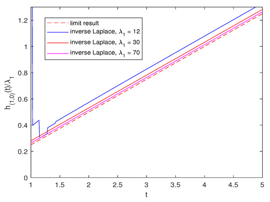
Thus, for , the number of collisions can be estimated as follows:
as
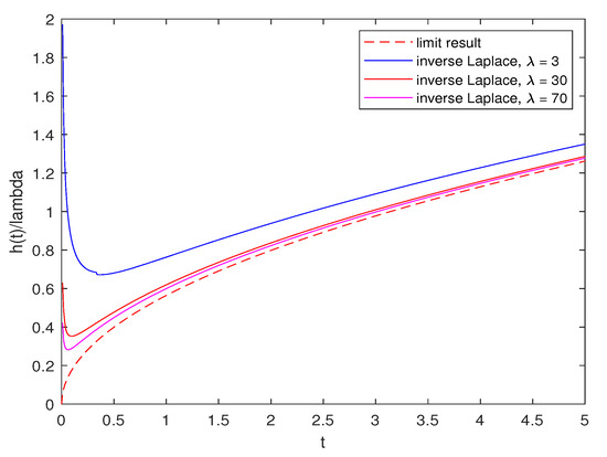
Now, if , that is , we have [16]
and
In this case, we have
The inverse Laplace transform with respect to s is
In Figure 2, we plot the numerical inverse transform of , including the asymptotic result that behaves as a function of .
4. Margrabe’s Spread Options Valuations with Two Telegraph Processes
There are many kinds of spread options. For instance, in the foreign exchange market (spread involves rates in different countries); in the fixed income market (spread between different maturities, e.g., in United States of America, it is Notes-Bonds (NOB) spread); there is also spread between quality levels, e.g., Treasury Bills-EuroDollars (TED spread); in the agricultural futures markets (e.g., soybean complex spread and corn spread); in the energy markets, there are crack spread options (e.g., gasoline crack spread, heating oil crack spread) or spark spread-converting a specific fuel (e.g., natural gas) into electricity. We can find this primary cross-commodity transaction in electric energy markets. For more details, see Carmona and Durrleman (2003) [10].
4.1. Recap: Margrabe’s Spread Options Valuations
Margrabe’s approach to spread option valuation is to price [17]
where and are two assets for spot prices under the risk-neutral measure, and they are modeled by two geometric Brownian motions (GBMs):
We denote by r the interest rate and T a maturity, and the correlation between the two Brownian motions and is a constant The change of numeraire is the most efficient method to solve this problem. Let us take as the numeraire. Then, in the Y measure, all assets discounted by Y must be martingales. Let be the value of the option at time Since V must be an martingale, we have:
from which we derive
We note that
We also note that the variance for the exponent in (20) is:
Since is log-normal distributed with variance we have:
where K is a strike price, and
For notational convenience, we denote for the “plus” sign, and for the “minus” sign.
We observe that there is no discounting because funding is embedded in the asset
Remark 1.
If we compare our result with the Black–Scholes formula, the value of the option of a call in Equation (23) is similar to BS as if we used BS with X as the underlying asset and as the strike price, with volatility We note that is the variance of
4.2. Two Telegraph Processes’ Dynamics
Let us have two telegraph processes on the real line with initial positions and
where is a velocity and are two independent Poisson processes with intensities and We can think about as the coordinates of two different particles on the real line at time
Each of the equations in (25) can be presented in the following equivalent form:
and
where are the sequences of Poisson times corresponding to each Poisson process and thus, or respectively.
We note that under different conditions for and , we will have different types of convergence for and :
Condition 1. Suppose that where is a constant.
According to the previous results, if and in such a manner that then converges weakly to the Wiener process ) with variance and converges weakly to the Wiener process with variance
when and and are two independent Wiener processes.
Condition 2. Suppose that and Condition 1 is not satisfied. Thus, we need once more Kac condition, besides for the weak convergence of namely we suppose that when and We note that, if this is the case, then:
and we assume that the two Wiener processes in (29) may be correlated with correlation
Remark 2.
Recent investigations of telegraph processes and their transformations were studied in [16,18,19].
4.3. Margrabe’s Spread Option Valuations with Two Telegraph Processes
In this subsection, we will evaluate spread option for two assets of spot prices modeled by two telegraph processes. We follow the approach presented in Section 4.1 above.
We use the following two GBM models for two assets:
We consider two cases below: (1) the dynamics for two assets in Equation (30) with Condition 1 and (2) the dynamics for two assets in (30) with Condition 2.
We used the geometric Brownian motion model or exponential model in (30) for a stock price to make the price positive.
4.4. Margrabe’s Valuations with Two Telegraph Processes under Condition 1
Suppose that Condition 1 in Section 4.2 is satisfied, i.e., where is a constant, and if and in such a manner that Thus, we approximate our volatilities in Equation (30) by and Therefore, the dynamics for two assets in (30) becomes:
Now, applying the method presented in Section 4.1, we have that the value of the spread option at time is given by:
where
4.5. Margrabe’s Valuations with Two Telegraph Processes under Condition 2
Suppose that Condition 2 in Section 4.2 is satisfied, i.e., and and when and
Now, we approximate our volatilities in (30) by and Therefore, the dynamics for two assets in (30) becomes:
where two Wiener processes in Equation (34) are correlated with correlation
Using the method presented in Section 4.1, the value of the spread option at time in this case is:
where
We note that Formulas (35) and (36) are more general than (32) and (33). For instance, if we take in (35) and (36), then we obtain exactly (32) and (33).
Remark 3.
Combining the two cases with Conditions 1 and 2 with correlated Wiener processes and , then we can obtain one more case, namely
where
Remark 4.
We should note that European call and put option pricing for stocks prices based on one telegraph process were studied in [16,18,19].
Remark 5.
In terms of market trading patterns, we can say that if the waiting time in each state for the process increases, then it will represent a low liquidity market, and vice versa, if the waiting time in each state decreases, then it will represent a high liquidity market. Furthermore, in a high-frequency and algorithmic trading market structure, our model for a stock price with telegraph process is more descriptive than the Black–Scholes model.
4.6. Numerical Results for Margrabe Valuations
In this section, we show some numerical examples of the behavior of for different three situations in Formulas (32), (35) and (37). We assume some typical data for etc. For instance, we present two plots of Equation (32) in Figure 3 by varying maturity T and two plots in Figure 4 by varying velocity v:
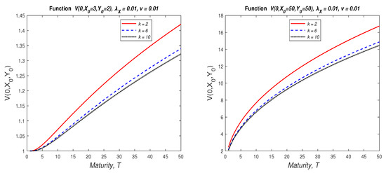
Figure 3.
Dependence of value of the option according to Equation (32) on maturity T for (left) and (right).
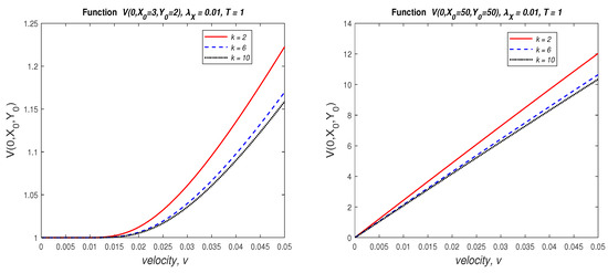
Figure 4.
Dependence of value of the option according to Equation (32) on velocity v for (left) and (right).
In Figure 5, we present two plots of Equation (35) by varying maturity T and two plots in Figure 6 by varying velocity v. In these plots, we also show variations of the correlation coefficient .
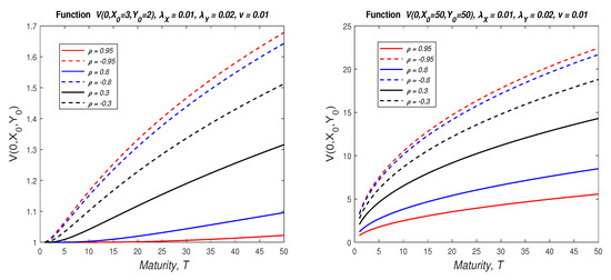
Figure 5.
Dependence of the value of the option according to Equation (35) on maturity T for (left) and (right).
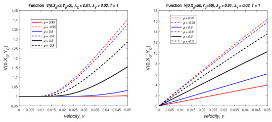
Figure 6.
Dependence of value of the option according to Equation (35) on velocity v for (left) and (right).
In Figure 7, we present two plots of Equation (37) by varying maturity T and correlation coefficient and two plots in Figure 8 by varying velocity v. In these plots, we also show variations of the correlation coefficient .
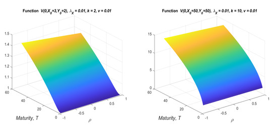
Figure 7.
Dependence of value of the option according to Equation (37) on maturity T and for and (left) and and (right).
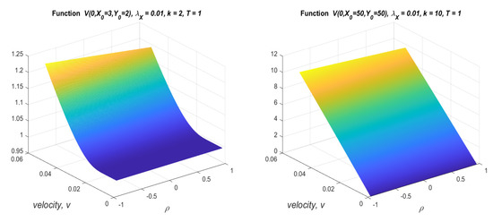
Figure 8.
Dependence of value of the option according to Equation (37) on velocity v and for and (left) and and (right).
5. Conclusions and Further Work
In this paper, we studied elastic collisions of two particles with independent random motion according to telegraph stochastic processes on the real line. We obtained an asymptotic estimation of the number of collisions under Kac’s condition for the cases where the direction-switching processes have the same parameters (symmetric) and different parameters (asymmetric). We applied numerical techniques for obtaining the inverse Laplace transform for the mean number of collisions of the two particles, and we found that such numerical results are consistent with the asymptotic result. As a continuation of this analysis, we may model collisions of multiple particles moving on the real line where each of them moves according to an independent telegraph process.
We also considered the financial application of these mathematical results to evaluate Margrabe’s spread option for two assets of spot prices.
Of course, our models for spread options valuation have some limitations associated with specific definitions of volatilities for both telegraph processes. Thus, our future work will be related to the comparative analysis of our model with other already existing models, such as Black–Scholes, jump-diffusion, etc. Another direction for our future work will be using real data to calibrate the parameters of the model, such as v, , and .
Author Contributions
Conceptualization, A.A.P., A.S. and R.M.R.-D.; Formal analysis, A.A.P., A.S. and R.M.R.-D.; Investigation, A.A.P., A.S. and R.M.R.-D.; Software, R.M.R.-D.; Writing—original draft, A.A.P.; Writing—review & editing, A.A.P., A.S. and R.M.R.-D. All authors have read and agreed to the published version of the manuscript.
Funding
This research was partiallt supported by NSERC (NSERC RT732266 project).
Institutional Review Board Statement
Not applicable.
Informed Consent Statement
Not applicable.
Data Availability Statement
Not applicable.
Acknowledgments
The second author thanks NSERC for the continuous support.
Conflicts of Interest
The authors declare no conflict of interest.
References
- Harris, T.E. Diffusion with “Collisions” between Particles. J. Appl. Probab. 1965, 2, 323–338. [Google Scholar] [CrossRef]
- Frank, S. Uniform Motion with Elastic Collision of an Infinite Particle System. J. Math. Mech. 1969, 18, 973–989. [Google Scholar]
- Peter, M.; Domokos, S. On the Effect of Collisions on the Motion of an Atom in R1. Ann. Probab. 1980, 8, 1068–1078. [Google Scholar]
- Kirk, E. Correlation in the Energy Markets. In Managing Energy Price Risk; Risk Publications and Enron: London, UK, 1995; pp. 71–78. [Google Scholar]
- Etesami, S.R. Spread Options: From Margrabe to Kirk. 2020. Available online: https://ssrn.com/abstract=3665654 (accessed on 31 May 2022). [CrossRef]
- Lo, C.-F. A Simple Derivation of Kirk’s Approximation for Spread Options. Appl. Math. Lett. 2013, 26, 904–907. [Google Scholar] [CrossRef]
- Neil, D. An Efficient Approach for Pricing Spread Options. 1999. Available online: https://ssrn.com/abstract=7010 (accessed on 31 May 2022).
- Choi, J. Sum of all Black–Scholes–Merton models: An efficient pricing method for spread, basket, and Asian options. J. Futur. Mark. 2018, 38, 627–644. [Google Scholar] [CrossRef]
- Li, M.; Deng, S.-J.; Zhou, J. Closed-Form Approximations for Spread Option Prices and Greeks. J. Deriv. Spring 2008, 15, 58–80. [Google Scholar] [CrossRef]
- Carmona, R.; Durrleman, V. Pricing and Hedging Spread Options; Working Paper; Princeton University: Princeton, NJ, USA, 2003. [Google Scholar]
- Pogorui, A.A.; Rodríguez-Dagnino, R.M. One-dimensional semi-Markov evolutions with general Erlang sojourn times. Random Oper. Stoch. Equ. 2005, 13, 399–405. [Google Scholar] [CrossRef][Green Version]
- Kolomiiets, T.; Pogorui, A.; Rodríguez-Dagnino, R.M. Solution of Systems of Partial Differential Equations by Using Properties of Monogenic Functions on Commutative Algebras. J. Math. Sci. 2019, 239, 43–50. [Google Scholar] [CrossRef]
- Cox, D.R. Renewal Theory, Published by Methuen; John Wiley & Sons: London, UK; New York, NY, USA, 1962. [Google Scholar]
- Korolyuk, V.S.; Limnios, N. Average and diffusion approximation for evolutionary systems in an asymptotic split phase space. Ann. Appl. Probab. 2004, 14, 489–516. [Google Scholar] [CrossRef]
- Kolesnik, A.D.; Ratanov, N. Telegraph Processes and Option Pricing; Springer: Heidelberg, Germany, 2013; Volume 204, p. 36. [Google Scholar]
- Pogorui, A.; Swishchuk, A.; Rodríguez-Dagnino, R.M. Random Motion in Markov and Semi-Markov Random Environment 1: Homogeneous and Inhomogeneous Random Motions; ISTE Ltd. & Wiley: London, UK, 2021; Volume 1. [Google Scholar]
- Margrabe, W. The value to exchange one asset for another. J. Financ. 1978, 33, 177–186. [Google Scholar] [CrossRef]
- Pogorui, A.; Swishchuk, A.; Rodríguez-Dagnino, R.M. Random Motion in Markov and Semi-Markov Random Environment 2: High-Dimensional Random Motions and Financial Applications; ISTE Ltd. & Wiley: London, UK, 2021; Volume 2. [Google Scholar]
- Pogorui, A.; Swishchuk, A.; Rodríguez-Dagnino, R.M. Transformations of Telegraph Processes and Their Financial Applications. Risks 2021, 9, 147. [Google Scholar] [CrossRef]


Publisher’s Note: MDPI stays neutral with regard to jurisdictional claims in published maps and institutional affiliations. |
© 2022 by the authors. Licensee MDPI, Basel, Switzerland. This article is an open access article distributed under the terms and conditions of the Creative Commons Attribution (CC BY) license (https://creativecommons.org/licenses/by/4.0/).