
Temperature Trend Analysis and Investigation on a Case of Variability Climate


Abstract
1. Introduction
2. Materials and Methods
2.1. Study Areas and Data Collection
2.2. Homogenization of Temperature Data
2.3. Trend Analysis Methods
3. Results
Clusters Descriptions
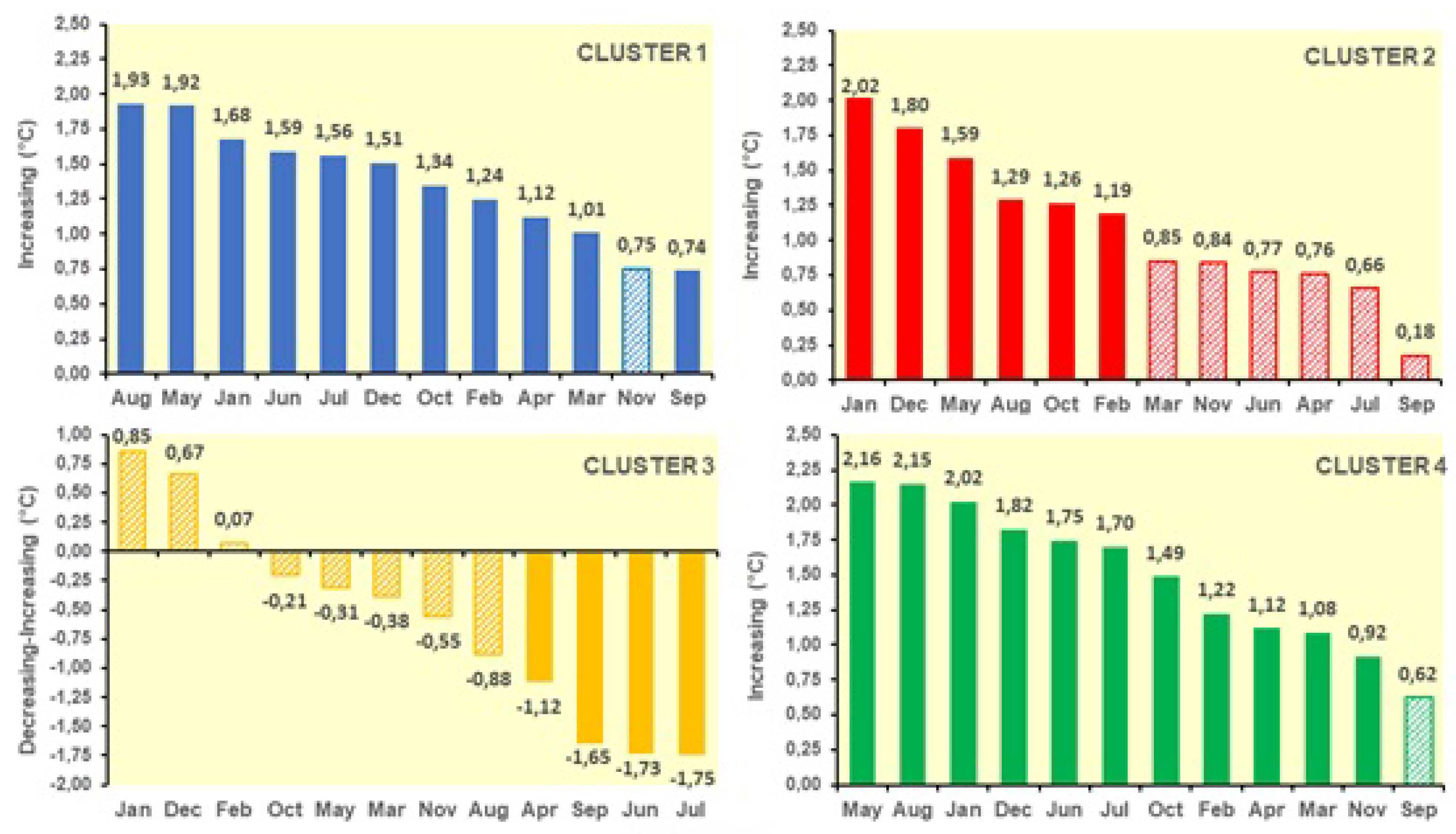
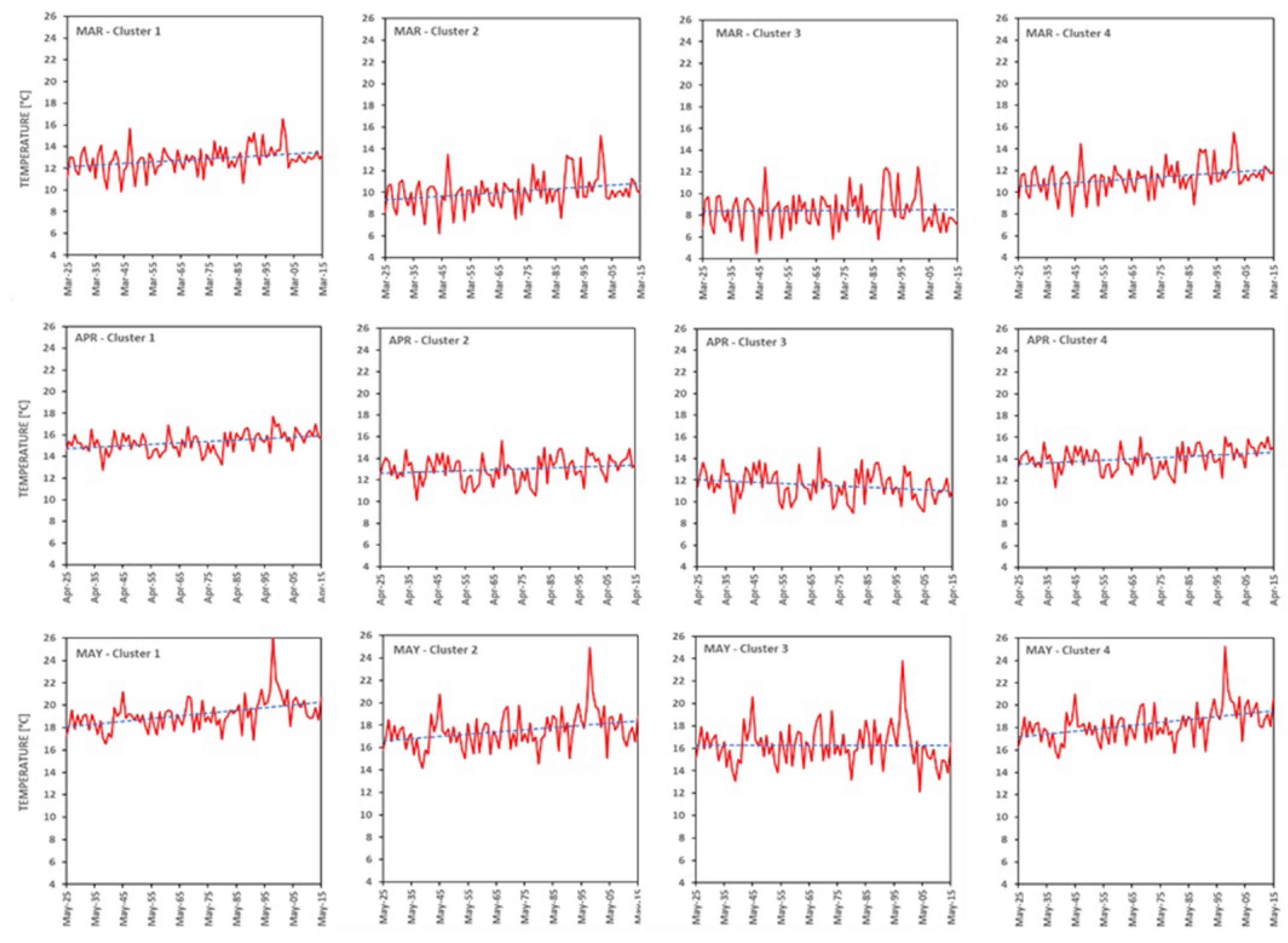
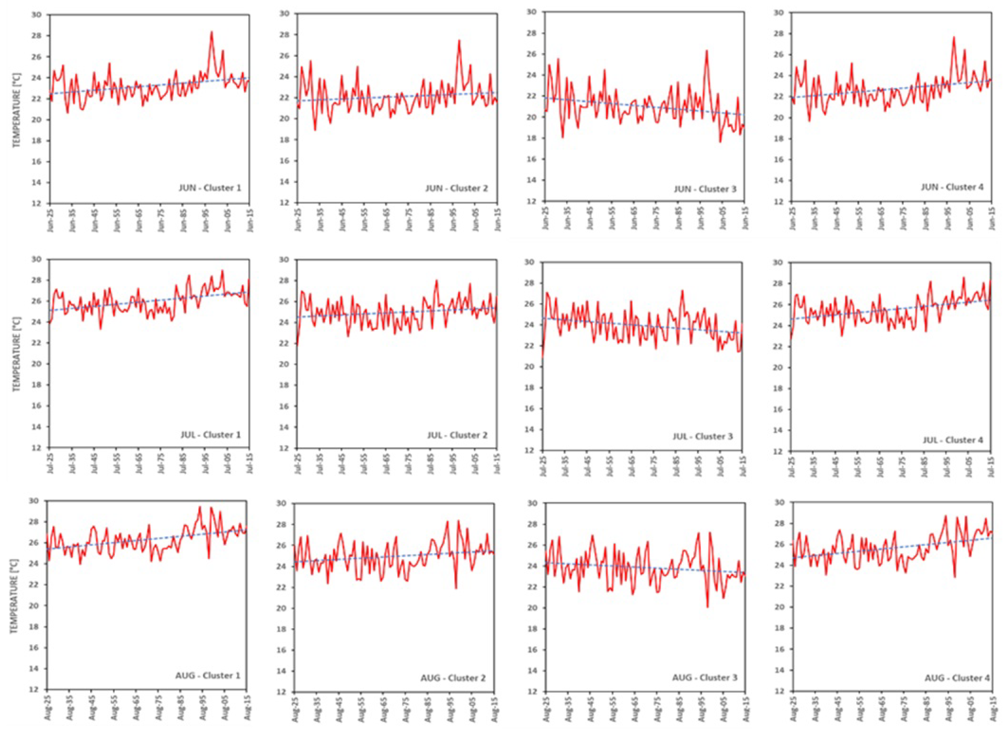
- Cluster 1: The results of the MKT highlight the significant presence of growing trends, regardless of the months of the year, with the exception of November. The null hypothesis is rejected, which means accepting the alternative hypothesis HA, or that there is a significant trend in the analyzed series. The sign of indicates an increasing trend. From Sen’s slope, it is possible to identify the months that experienced the highest rate of temperature increase. August and May are those that undergo the highest increase, exceeding 1.9 °C. Significant is the month of January where the increase approaches 1.7 °C. The months of June and July show an increase close to 1.6 °C. Another significant month with an increase of 1.5 °C is December. The increases for the months of October, February, April and March instead oscillate between 1.3 °C and 1.0 °C. The months of November, in which no trend was identified; vice versa, September underwent the lowest increase, about 0.7 °C.
- Cluster 2: A double behavior is evident, six months show increasing trends while during the other six months no significant trend has been observed, having accepted the null hypothesis . From the Sen’s slope it is clear that the months of January and December are those that have undergone the greatest increase in temperature, respectively 2.0 °C and 1.8 °C. The month of May shows an increase of 1.6 °C, while the increase in August, October, February oscillates between 1.3 °C and 1.2 °C. The remaining six months show no obvious trends; their increase does not exceed 0.8 °C.
- Cluster 3: Based on the results of MKT and in accordance with the sign of , there are decreasing trends in temperatures in the months of April, September, June and July; for the remaining months no trend was observed as the null hypothesis is accepted. The Sen slope shows a significant decrease in temperature in the months of June and July with −1.7 °C. September follows with −1.6 °C and April with −1.1 °C. In the remaining months, although there are no significant trends, there was a decrease between −0.2 °C and −0.9 °C, while in the months of January and December there were increases of +0.8 °C and +0.7 °C, respectively.
- Cluster 4: Growing trends are well highlighted by the results of the MKT and in accordance with the sign of , regardless of the months of the year, with the exception of September in which the null hypothesis is accepted. From the Sen’s slope the highest temperature increase is found in the months of May and August, respectively 2.2 °C and 2.1 °C. Particularly significant is the increase in the months of January and December, 2.0 °C and 1.8 °C respectively. In the months of June and July there is an increase of 1.7 °C. As for the months of February, March, April, October, the increase oscillates between 1.0 °C and 1.5 °C. The month of November, followed by the month of September in which no significant trend is observed, shows increases of 0.9 °C and 0.6 °C, respectively.
4. Discussion
5. Conclusions
Author Contributions
Funding
Institutional Review Board Statement
Informed Consent Statement
Data Availability Statement
Acknowledgments
Conflicts of Interest
References
- Vicente-Serrano, S.M.; Lopez-Moreno, J.I.; Beguería, S.; Lorenzo-Lacruz, J.; Sanchez-Lorenzo, A.; García-Ruiz, J.M.; Azorin-Molina, C.; Morán-Tejeda, E.; Revuelto, J.; Trigo, R.; et al. Evidence of increasing drought severity caused by temperature rise in southernEurope. Environ. Res. Lett. 2014, 9, 044001. [Google Scholar] [CrossRef]
- Lionello, P.; Scarascia, L. The relation between climate change in the Mediterranean region and global warming. Reg. Environ. Chang. 2018, 18, 1481–1493. [Google Scholar] [CrossRef]
- Lionello, P.; Abrantes, F.; Gacic, M.; Planton, S.; Trigo, R.; Ulbrich, U. The climate of the Mediterranean region: Research progress and climate change impacts. Reg. Environ. Chang. 2014, 14, 1679–1684. [Google Scholar] [CrossRef]
- Monforte, P.; Ragusa, M.A. Evaluation of the air pollution in a Mediterranean region by the air quality index. Environ. Monit. Assess. 2018, 190, 625. [Google Scholar] [CrossRef]
- Linares, C.; Díaz, J.; Negev, M.; Martínez, G.S.; Debono, R.; Paz, S. Impacts of climate change on the public health of the Mediterranean Basin population-current situation, projections, preparedness and adaptation. Environ. Res. 2020, 182, 109107. [Google Scholar] [CrossRef] [PubMed]
- Hochman, A.; Alpert, P.; Baldi, M.; Bucchignani, E.; Coppola, E.; Dahdal, Y.; Davidovitch, N.; Georgiades, P.; Helgert, S.; Khreis, H.; et al. Interdisciplinary Regional Collaboration for Public Health Adaptation to Climate Change in the Eastern Mediterranean. Bull. Am. Meteorol. Soc. 2020, 101, E1685–E1689. [Google Scholar] [CrossRef]
- Klausmeyer, K.R.; Shaw, M.R. Climate change, habitat loss, protected areas and the climate adaptation potential of species in Mediterranean ecosystems worldwide. PLoS ONE 2009, 4, e6392. [Google Scholar] [CrossRef]
- Iglesias, A.; Mougou, R.; Moneo, M.; Quiroga, S. Towards adaptation of agriculture to climate change in the Mediterranean. Reg. Environ. Chang. 2011, 11, 159–166. [Google Scholar] [CrossRef]
- Evans, A.; Perschel, R. A review of forestry mitigation and adaptation strategies in the Northeast U.S. Clim. Chang. 2009, 96, 167–183. [Google Scholar] [CrossRef]
- Huppmann, D.; Rogelj, J.; Kriegler, E.; Krey, V.; Riahi, K. A new scenario resource for integrated 1.5 C research. Nat. Clim. Chang. 2018, 8, 1027–1030. [Google Scholar] [CrossRef]
- IPCC-Report. 2018. Available online: http://www.ipcc-data.org/guidelines/pages/definitions.html (accessed on 1 March 2022).
- European Commission. Communication from the Commission: A Clean Planet for All. A European Strategic Long-Term Vision for a Prosperous, Modern, Competitive and Climate Neutral Economy; COM(2018) 773 Final; European Commission: Brussels, Belgium, 2018. [Google Scholar]
- Caloiero, T.; Coscarelli, R.; Ferrari, E.; Sirangelo, B. Trend analysis of monthly mean values and extreme indices of daily temperature in a region of southern Italy. Int. J. Climatol. 2017, 37, 284–297. [Google Scholar] [CrossRef]
- Cheshmehzangi, A. The analysis of global warming patterns from 1970s to 2010s. Atmos. Clim. Sci. 2020, 10, 392–404. [Google Scholar] [CrossRef]
- Zahradníček, P.; Brázdil, R.; Štěpánek, P.; Trnka, M. Reflections of global warming in trends of temperature characteristics in the Czech Republic, 1961–2019. Int. J. Climatol. 2021, 41, 1211–1229. [Google Scholar] [CrossRef]
- Trbic, G.; Popov, T.; Gnjato, S. Analysis of air temperature trends in Bosnia and Herzegovina. Geogr. Pannonica 2017, 21, 68–84. [Google Scholar] [CrossRef]
- Ukey, R.; Rai, A.C. Impact of global warming on heating and cooling degree days in major Indian cities. Energy Build. 2021, 244, 111050. [Google Scholar] [CrossRef]
- Lanzafame, R.; Monforte, P.; Scandura, P.F. Comparative analyses of urban air quality monitoring systems: Passive sampling and continuous monitoring stations. Energy Procedia 2016, 101, 321–328. [Google Scholar]
- Ward, J.H., Jr. Hierarchical Grouping to Optimize an Objective Function. J. Am. Stat. Assoc. 1963, 58, 236–244. [Google Scholar] [CrossRef]
- Gavioli, A.; de Souza, E.G.; Bazzi, C.L.; Schenatto, K.; Betzek, N.M. Identification of management zones in precision agriculture: An evaluation of alternative cluster analysis methods. Biosyst. Eng. 2019, 181, 86–102. [Google Scholar] [CrossRef]
- Brusca, S.; Famoso, F.; Lanzafame, R.; Messina, M.; Monforte, P. Placement optimization of biodiesel production plant by means of centroid mathematical method. Energy Procedia 2017, 126, 353–360. [Google Scholar] [CrossRef]
- Dell’Aquila, A.; Calmanti, S. Evaluation of Climate Patterns in a Regional Climate Model over Italy Using Long-Term Records from SYNOP Weather Stations and Cluster Analysis. Clim. Res. 2015, 62, 173–188. [Google Scholar]
- Munoz-Diaz, D.; Rodrigo, F.S. Spatio-Temporal Patterns of Seasonal Rainfall in Spain (1912–2000) Using Cluster and Principal Component Analysis: Comparison. In Annales Geophysicae; Copernicus GmbH: Göttingen, Germany, 2004; Volume 22. [Google Scholar]
- Pérez-Zanón, N.; Sigró, J.; Domonkos, P.; Ashcroft, L. Comparison of HOMER and ACMANT homogenization methods using a central Pyrenees temperature dataset. Adv. Sci. Res. 2015, 12, 111–119. [Google Scholar] [CrossRef]
- Unal, Y.; Tayfun, K.; Mehmet, K. Redefining the climate zones of Turkey using cluster analysis. Int. J. Climatol. A J. R. Meteorol. Soc. 2003, 23, 1045–1055. [Google Scholar] [CrossRef]
- Mann, H.B. Nonparametric tests against trend. Econom. J. Econom. Soc. 1945, 13, 245–259. [Google Scholar] [CrossRef]
- Kendall, M.G. Rank Correlation Methods; Griffin, American Psicological Association: Washington, DC, USA, 1948. [Google Scholar]
- Yusuf, A.S.; Edet, C.O.; Oche, C.O.; Agbo, E.P. Trend analysis of temperature in Gombe state using Mann Kendall trend test. J. Sci. Res. Rep. 2018, 20, 1–9. [Google Scholar]
- Yadav, R.; Tripathi, S.K.; Pranuthi, G.; Dubey, S.K. Trend analysis by Mann-Kendall test for precipitation and temperature for thirteen districts of Uttarakhand. J. Agrometeorol. 2014, 16, 164. [Google Scholar] [CrossRef]
- Yue, S.; Pilon, P.; Phinney, B.; Cavadias, G. The influence of autocorrelation on the ability to detect trend in hydrological series. Hydrol. Process. 2002, 16, 1807–1829. [Google Scholar] [CrossRef]
- Robaa, E.-S.M.; Al-Barazanji, Z. Mann-Kendall trend analysis of surface air temperatures and rainfall in Iraq. Q. J. Hung. Meteorol. Serv. 2015, 119, 493–514. [Google Scholar]
- Modarres, R.; da Silva, V.P.R. Rainfall trends in arid and semi-arid regions of Iran. J. Arid Environ. 2007, 70, 344–355. [Google Scholar] [CrossRef]
- Partal, T.; Kahya, E. Trend analysis in Turkish precipitation data. Hydrol. Process. Int. J. 2006, 20, 2011–2026. [Google Scholar] [CrossRef]
- Famoso, F.; Lanzafame, R.; Monforte, P.; Oliveri, C.; Scandura, P.F. Air quality data for Catania: Analysis and investigation case study 2012–2013. Energy Procedia 2015, 81, 644–654. [Google Scholar] [CrossRef][Green Version]
- Sen, P.K. Estimates of the regression coefficient based on Kendall’s tau. J. Am. Stat. Assoc. 1968, 63, 1379–1389. [Google Scholar] [CrossRef]
- Lettenmaier, D.P.; Wood, E.F.; Wallis, J.R. Hydro-climatological trends in the continental United States, 1948–1988. J. Clim. 1994, 7, 586–607. [Google Scholar] [CrossRef]
- Yue, S.; Hashino, M. Temperature trends in Japan: 1900–1996. Theor. Appl. Climatol. 2003, 75, 15–27. [Google Scholar] [CrossRef]
- He, Y.; Yiping, Z. Climate change from 1960 to 2000 in the Lancang River Valley, China. Mt. Res. Dev. 2005, 25, 341–348. [Google Scholar]
- El-Nesr, M.N.; Majed, M.A.-Z.; Alazba, A.A. Temperature trends and distribution in the Arabian Peninsula. Am. J. Environ. Sci. 2010, 6, 191–203. [Google Scholar] [CrossRef]
- Viola, F.; Liuzzo, L.; Noto, L.V.; Lo Conti, F.; La Loggia, G. Spatial distribution of temperature trends in Sicily. Int. J. Climatol. 2014, 34, 1–17. [Google Scholar] [CrossRef]
- Brusca, S.; Famoso, F.; Lanzafame, R.; Garrano, A.M.C.; Monforte, P. Experimental analysis of a plume dispersion around obstacles. Energy Procedia 2015, 82, 695–701. [Google Scholar] [CrossRef]
- Fratianni, S.; Acquaotta, F. The climate of Italy. In Landscapes and Landforms of Italy; Springer: Cham, Switzerland, 2017; pp. 29–38. [Google Scholar]
- Pinna, M. Contributi di Climatologia; Memorie della Sociéta Geografica Italiana: Roma, Italy, 1985; Volume 39. [Google Scholar]
- Sugar, C.A.; Gareth, M.J. Finding the number of clusters in a dataset: An information-theoretic approach. J. Am. Stat. Assoc. 2003, 98, 750–763. [Google Scholar] [CrossRef]
- Hipel, K.W.; McLeod, A.I. Time Series Modelling of Water Resources and Environmental Systems; Elsevier: Amsterdam, The Netherlands, 1994. [Google Scholar]
- Duro, A.; Piccione, V.; Ragusa, M.A.; Rapicavoli, V.; Veneziano, V. Enviromentally sensitive patch index of desertification risk applied to the main habitats of Sicily. In AIP Conference Proceedings; American Institute of Physics: College Park, MD, USA, 2017; Volume 1863. [Google Scholar]
- Duro, A.; Piccione, V.; Ragusa, M.A.; Veneziano, V. New enviromentally sensitive patch index-ESPI-for MEDALUS protocol. In AIP Conference Proceedings; American Institute of Physics: College Park, MD, USA, 2014; Volume 1637. [Google Scholar]
- Duro, A.; Piccione, V.; Ragusa, M.A.; Rapicavoli, V.; Veneziano, V. The environmentally sensitive index patch applied to MEDALUS climate quality index. In AIP Conference Proceedings; American Institute of Physics: College Park, MD, USA, 2016; Volume 1738. [Google Scholar]
- Tabari, H.; Marofi, S.; Aeini, A.; Talaee, P.H.; Mohammadi, K. Trend analysis of reference evapotranspiration in the western half of Iran. Agric. For. Meteorol. 2011, 151, 128–136. [Google Scholar] [CrossRef]
- Shadmani, S.S.; Marofi, S.; Roknian, M. Trend analysis in reference evapotranspiration using Mann-Kendall and Spearman’s Rho tests in arid regions of Iran. Water Resour. Manag. 2012, 26, 211–224. [Google Scholar] [CrossRef]
- Tabari, H.; Talaee, P.H. Analysis of trends in temperature data in arid and semi-arid regions of Iran. Glob. Planet. Chang. 2011, 79, 1–10. [Google Scholar] [CrossRef]
- Arnone, E.; Cucchi, M.; Gesso, S.D.; Petitta, M.; Calmanti, S. Droughts prediction: A methodology based on climate seasonal forecasts. Water Resour. Manag. 2020, 34, 4313–4328. [Google Scholar] [CrossRef]
- Bordi, I.; Sutera, A. An analysis of drought in Italy in the last fifty years. Il Nuovo Cimento C 2002, 25, 185–206. [Google Scholar]


| Month | Number Obs. | Min | Max | Mean | Std. Dev. | Statistic (Zs) | p-Value | Sen’s Slope | Test Interpretation ( = 0.05) | Trend | |
|---|---|---|---|---|---|---|---|---|---|---|---|
| CLUSTER 1 | Jan | 90 | 7812 | 13,615 | 11,052 | 1152 | +4273 | <0.0001 | 0.019 | Reject H0 | Increasing |
| Feb | 90 | 8055 | 14,167 | 11,249 | 1313 | +2412 | 0.0159 | 0.014 | Reject H0 | Increasing | |
| Mar | 90 | 9831 | 16,558 | 12,852 | 1168 | +2774 | 0.0055 | 0.011 | Reject H0 | Increasing | |
| Apr | 90 | 12,724 | 17,701 | 15,321 | 0936 | +3248 | 0.0012 | 0.012 | Reject H0 | Increasing | |
| May | 90 | 16,558 | 25,997 | 19,200 | 1394 | +4461 | < 0.0001 | 0.021 | Reject H0 | Increasing | |
| Jun | 90 | 20,645 | 28,420 | 23,249 | 1288 | +3304 | 0.0010 | 0.018 | Reject H0 | Increasing | |
| Jul | 90 | 23,295 | 28,966 | 26,022 | 1099 | +3869 | 0.0001 | 0.017 | Reject H0 | Increasing | |
| Aug | 90 | 23,954 | 29,451 | 26,302 | 1172 | +4583 | < 0.0001 | 0.021 | Reject H0 | Increasing | |
| Sep | 90 | 20,783 | 26,464 | 23,545 | 1015 | +2140 | 0.0324 | 0.008 | Reject H0 | Increasing | |
| Oct | 90 | 15,297 | 22,897 | 19,758 | 1360 | +2593 | 0.0095 | 0.015 | Reject H0 | Increasing | |
| Nov | 90 | 12,215 | 18,213 | 15,762 | 1062 | +1791 | 0.0732 | 0.008 | Acept H0 | No Trend | |
| Dec | 90 | 9203 | 19,672 | 12,683 | 1653 | +3534 | 0.0004 | 0.017 | Reject H0 | Increasing | |
| CLUSTER 2 | Jan | 90 | 4096 | 10,516 | 7768 | 1351 | +4308 | < 0.0001 | 0.022 | Reject H0 | Increasing |
| Feb | 90 | 4045 | 12,407 | 8108 | 1622 | +1969 | 0.0489 | 0.013 | Reject H0 | Increasing | |
| Mar | 90 | 6174 | 15,248 | 10,100 | 1503 | +1805 | 0.0710 | 0.009 | Acept H0 | No Trend | |
| Apr | 90 | 10,134 | 15,633 | 12,999 | 1191 | +1757 | 0.0790 | 0.008 | Acept H0 | No Trend | |
| May | 90 | 14,170 | 24,923 | 17,516 | 1646 | +2997 | 0.0027 | 0.018 | Reject H0 | Increasing | |
| Jun | 90 | 18,908 | 27,480 | 22,107 | 1448 | +1534 | 0.1252 | 0.009 | Acept H0 | No Trend | |
| Jul | 90 | 22,653 | 28,072 | 24,990 | 1203 | +1342 | 0.1797 | 0.007 | Acept H0 | No Trend | |
| Aug | 90 | 21,867 | 28,377 | 24,944 | 1384 | +2475 | 0.0133 | 0.014 | Reject H0 | Increasing | |
| Sep | 90 | 18,168 | 25,063 | 21,397 | 1257 | +0397 | 0.6911 | 0.002 | Acept H0 | No Trend | |
| Oct | 90 | 11,994 | 21,236 | 17,003 | 1602 | +2112 | 0.0347 | 0.014 | Reject H0 | Increasing | |
| Nov | 90 | 8426 | 16,191 | 12,629 | 1249 | +1624 | 0.1043 | 0.009 | Acept H0 | No Trend | |
| Dec | 90 | 5130 | 17,319 | 9434 | 1834 | +3966 | < 0.0001 | 0.020 | Reject H0 | Increasing | |
| CLUSTER 3 | Jan | 90 | 2334 | 8863 | 5937 | 1411 | +1603 | 0.1089 | 0.009 | Acept H0 | No Trend |
| Feb | 90 | 1772 | 11,534 | 6348 | 1873 | +0091 | 0.9278 | 0.001 | Acept H0 | No Trend | |
| Mar | 90 | 4469 | 12,494 | 8477 | 1628 | −0760 | 0.4474 | −0.004 | Acept H0 | No Trend | |
| Apr | 90 | 8941 | 15,000 | 11,523 | 1351 | −2164 | 0.0304 | −0.012 | Reject H0 | Decreasing | |
| May | 90 | 12,150 | 23,806 | 16,286 | 1789 | −0488 | 0.6256 | −0.003 | Acept H0 | No Trend | |
| Jun | 90 | 17,600 | 26,366 | 21,043 | 1680 | −2792 | 0.0052 | −0.019 | Reject H0 | Decreasing | |
| Jul | 90 | 21,438 | 27,319 | 23,977 | 1414 | −3109 | 0.0019 | −0.019 | Reject H0 | Decreasing | |
| Aug | 90 | 20,041 | 27,225 | 23,831 | 1536 | −1446 | 0.1481 | −0.010 | Acept H0 | No Trend | |
| Sep | 90 | 16,359 | 24,116 | 20,002 | 1549 | −2684 | 0.0073 | −0.018 | Reject H0 | Decreasing | |
| Oct | 90 | 9984 | 19,688 | 15,367 | 1676 | −0272 | 0.7857 | −0.002 | Acept H0 | No Trend | |
| Nov | 90 | 6209 | 15,256 | 10,856 | 1323 | −1046 | 0.2958 | −0.006 | Acept H0 | No Trend | |
| Dec | 90 | 3278 | 15,797 | 7606 | 1954 | +1209 | 0.2265 | 0.007 | Acept H0 | No Trend | |
| CLUSTER 4 | Jan | 90 | 5711 | 11,658 | 9245 | 1241 | +4635 | < 0.0001 | 0.022 | Reject H0 | Increasing |
| Feb | 90 | 5819 | 13,209 | 9529 | 1458 | +2171 | 0.0299 | 0.014 | Reject H0 | Increasing | |
| Mar | 90 | 7775 | 15,515 | 11,356 | 1328 | +2872 | 0.0041 | 0.012 | Reject H0 | Increasing | |
| Apr | 90 | 11,349 | 16,062 | 14,071 | 1080 | +2708 | 0.0068 | 0.012 | Reject H0 | Increasing | |
| May | 90 | 15,240 | 25,240 | 18,347 | 1532 | +4259 | < 0.0001 | 0.024 | Reject H0 | Increasing | |
| Jun | 90 | 19,636 | 27,694 | 22,721 | 1404 | +3416 | 0.0006 | 0.019 | Reject H0 | Increasing | |
| Jul | 90 | 22,979 | 28,604 | 25,561 | 1217 | +3478 | 0.0005 | 0.019 | Reject H0 | Increasing | |
| Aug | 90 | 22,832 | 28,762 | 25,649 | 1351 | +4085 | < 0.0001 | 0.024 | Reject H0 | Increasing | |
| Sep | 90 | 19,138 | 25,513 | 22,406 | 1163 | +1499 | 0.1340 | 0.007 | Acept H0 | No Trend | |
| Oct | 90 | 13,213 | 21,604 | 18,263 | 1509 | +2642 | 0.0082 | 0.017 | Reject H0 | Increasing | |
| Nov | 90 | 9809 | 17,026 | 14,039 | 1181 | +1973 | 0.0485 | 0.010 | Reject H0 | Increasing | |
| Dec | 90 | 6962 | 18,294 | 10,895 | 1724 | +4133 | < 0.0001 | 0.020 | Reject H0 | Increasing |
| Month | Cluster 1 | Cluster 2 | Cluster 3 | Cluster 4 |
|---|---|---|---|---|
| Jan | +1.68 | +2.02 | +0.85 | +2.02 |
| Feb | +1.24 | +1.19 | +0.07 | +1.22 |
| Mar | +1.01 | +0.85 | −0.38 | +1.08 |
| Apr | +1.12 | +0.76 | −1.12 | +1.12 |
| May | +1.92 | +1.59 | −0.31 | +2.16 |
| Jun | +1.59 | +0.77 | −1.73 | +1.75 |
| Jul | +1.56 | +0.66 | −1.75 | +1.70 |
| Aug | +1.93 | +1.29 | −0.88 | +2.15 |
| Sep | +0.74 | +0.18 | −1.65 | +0.62 |
| Oct | +1.34 | +1.26 | −0.21 | +1.49 |
| Nov | +0.75 | +0.84 | −0.55 | +0.92 |
| Dec | +1.51 | +1.80 | +0.67 | +1.82 |
Publisher’s Note: MDPI stays neutral with regard to jurisdictional claims in published maps and institutional affiliations. |
© 2022 by the authors. Licensee MDPI, Basel, Switzerland. This article is an open access article distributed under the terms and conditions of the Creative Commons Attribution (CC BY) license (https://creativecommons.org/licenses/by/4.0/).
Share and Cite
Monforte, P.; Ragusa, M.A. Temperature Trend Analysis and Investigation on a Case of Variability Climate. Mathematics 2022, 10, 2202. https://doi.org/10.3390/math10132202
Monforte P, Ragusa MA. Temperature Trend Analysis and Investigation on a Case of Variability Climate. Mathematics. 2022; 10(13):2202. https://doi.org/10.3390/math10132202
Chicago/Turabian StyleMonforte, Pietro, and Maria Alessandra Ragusa. 2022. "Temperature Trend Analysis and Investigation on a Case of Variability Climate" Mathematics 10, no. 13: 2202. https://doi.org/10.3390/math10132202
APA StyleMonforte, P., & Ragusa, M. A. (2022). Temperature Trend Analysis and Investigation on a Case of Variability Climate. Mathematics, 10(13), 2202. https://doi.org/10.3390/math10132202