Hybrid LSTM-ARMA Demand-Forecasting Model Based on Error Compensation for Integrated Circuit Tray Manufacturing

Abstract

Demand forecasting plays a crucial role in a company’s operating costs. Excessive inventory can increase costs and unnecessary waste can be reduced if managers plan for uncertain future demand and determine the most favorable decisions. Managers are demanding increasing accuracy in forecasting as technology advances. Most of the literature discusses forecasting results’ inaccuracy by suspending the model and reloading the data for model retraining and correction, which is extensively employed but causes a bottleneck in practice since users do not have the sufficient ability to correct the model. This study proposes an error compensation mechanism and uses the individuals and moving-range (I-MR) control chart to evaluate the requirement for compensation to solve the current bottleneck using forecasting models. The approach is validated using the case companies’ historical data, and the model is developed using a rolling long short-term memory (LSTM) to output the predicted values; then, five indicators are proposed for screening to determine the prediction statistics to be subsequently employed. Root mean squared error (RMSE), mean absolute percentage error (MAPE), and mean absolute error (MAE) compare the LSTM, rolling LSTM combined index, and LSTM-autoregressive moving average (ARMA) models. The results demonstrate that the RMSE, MAPE, and MAE of LSTM-ARMA are smaller than those of the other two models, indicating that the error compensation mechanism that is proposed in this study can enhance the prediction’s accuracy.

1. Introduction

Companies are finding it difficult to accurately forecast customer demand using traditional demand-forecasting approaches, preferring to employ data science approaches for demand-forecasting modeling due to the explosion of competition and information technology in the market [1,2]. Companies can use predictive analytics to respond to changes in future market trends to enhance their competitive advantage. Predictive analytics is a critical tool for understanding future needs. Since customer demand is the basis for all activity planning, it is time-varying. Thus, accurate demand forecasting will prevent stock-outs and increase customer satisfaction [3].

In lean manufacturing, inventory is one of the significant wastes. Inventory is a major bottleneck in a company’s operating costs. Demand forecasting can reduce inventory, so establishing an accurate demand-forecasting system is a primary objective for enhancing competitiveness. Demand forecasting has been used in various fields, such as electricity demand forecasting [4], tourism demand forecasting [5,6], restaurant demand forecasting [7], oil production forecasting [8], and stock market forecasting [9]. Most of them can initially attain the expected accuracy using statistical approaches or machine learning models, but after some time, they fail to generate the expected answers due to over-reliance on time. The most crucial aspect of forecasting is to respond effectively to trends, and managers focus on continually reducing the error between forecast and actual values. To enhance forecast accuracy, the development of models overtime is necessary. Thus, rolling forecasts are crucial steps to facilitate model correction. The error in the rolling prediction increases with the number of prediction steps due to white noise in the time series, causing the prediction to deteriorate with the number of steps. The error compensation approach employs historical forecast error to correct the future forecast values based on multi-step forecasting to compensate for each forecasted error value [10]. Furthermore, the air quality index (AQI) indicator only provides current forecasts and cannot provide valid values for those who will be outdoors in the next few hours. Liang et al. proposed a rolling AQI prediction model for the next 6 h for seven air quality regions in Taiwan using characteristic curves [11]. The mean absolute normalized coarse-error margins for rolling forecasts are all below 9%. The results demonstrate that a rolling forecast model that is built using the monthly characteristic curve can produce highly accurate forecasts.

The COVID-19 pandemic has triggered a global public health crisis, forcing many to work from home [12]. In this globally connected world, every country will be affected by the disruption that has been caused by the pandemic. This has led to total lockdowns in many countries around the world. In this case, all business activities in all industries have come to a complete halt. With social restrictions and closing city gates to prevent the epidemic spread of the virus, companies have launched strategies such as remote office working and video conferencing [13]. Therefore, the demand for notebook computers and tablet computers has also increased.

Integrated circuit (IC) trays have a protective effect on electronic products’ packaging. During packaging and testing, the IC components are placed in trays and then placed into test machines for testing. IC trays are one of the indispensable materials for precision parts IC components packaging tools, as well as a necessity for packaging and testing. The demand for plastic IC trays has grown with the electronics industry’s development [14]. In addition to supply and demand factors, the price of plastic raw materials is closely related to oil. COVID-19, supply–demand imbalances, and volatility in international financial markets are all associated with global oil demand, as is the collapse in the industrial feedstock oil’s price. However, price fluctuations can offer some gains or risks to the economies in the relevant chain. The related relevant chain includes raw material for IC trays (modified polyphenylene oxide), as well as packaging and testing manufacturers. Therefore, the Organization of Petroleum Exporting Countries member countries and allies have met to negotiate production cuts to save oil prices. However, the breakdown of negotiations between Saudi Arabia and Russia increased oil volumes instead of decreasing them, causing an oil price war that brought oil prices to a new low, affecting the prices of plasticized products [15]. If we can predict IC tray demand, we can purchase raw materials at low prices to reduce costs and increase profits, which becomes an advantage of low-price inventory and can react rapidly to market changes.

The demand for IC trays has been increasing due to various strategies adopted by various countries to combat the epidemic. The price of raw materials for producing IC trays has changed because of the unstable international situation arising from different external factors. Thus, if we know the demand for IC trays in advance, we can purchase the number of raw materials that are required to produce them in advance, in order to rapidly respond to the changes in market demand and maintain the competitiveness of our company. Manufacturers’ requirements for the accuracy of forecast results are increasing as information technology improves. Companies can reduce costs, increase profits, and enhance customer satisfaction by improving demand-forecasting accuracy. Thus, this study proposes an error compensation mechanism that captures nonlinear data with a rolling long short-term memory (LSTM) and then compensates for the residuals with the rolling autoregressive moving average (ARMA) model, which can only reduce the forecasting model’s maintenance cost and reduce the time for model correction and training.

2. Materials and Methods

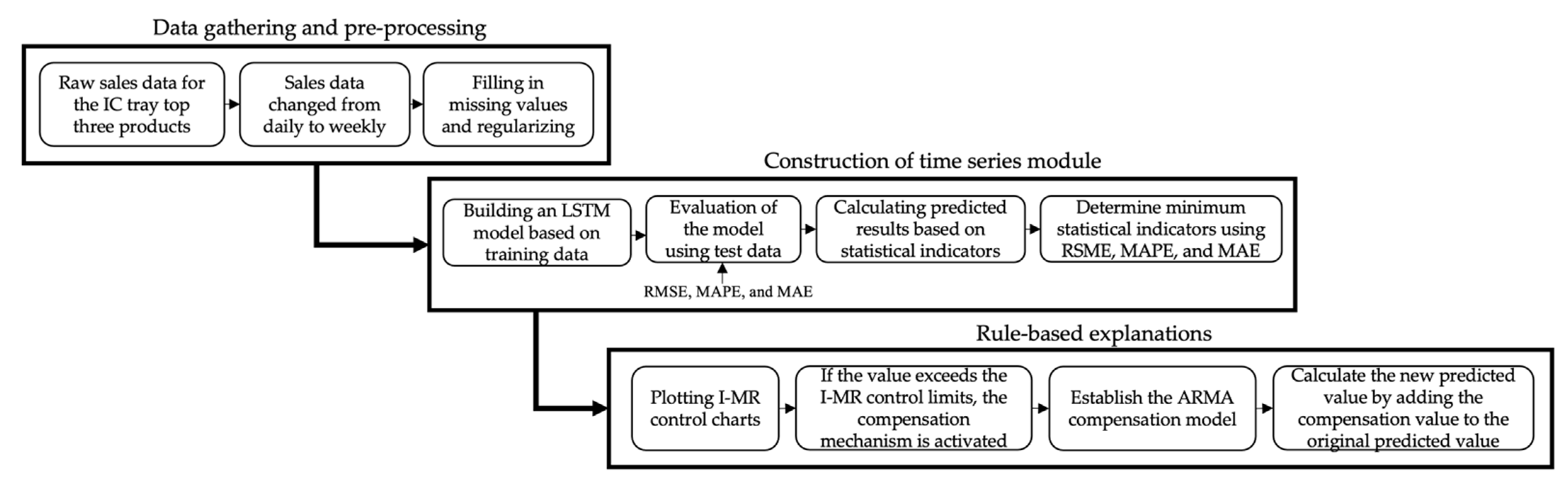
In this study, we propose a solution for an IC tray manufacturer’s data characteristics in Taiwan using industry–academia cooperation as an example, and verify the method’s feasibility. Recently, manufacturers of IC trays have been moving toward a less sample, more volume model, as customers’ requirements for IC shapes and sizes frequently change due to product diversification. The IC tray industry’s service characteristics emphasize order acceptance and speed of delivery, resulting in shorter production times. To reduce demand uncertainty’s impact and risk caused by market fluctuations, a systematic and highly accurate demand-forecasting model to assist in decision-making is urgently needed. The flowchart shown in Figure 1 was designed to include data gathering and pre-processing, the construction of a time series module, and rule-based explanations.

Figure 1. The analysis framework flowchart.

2.1. Data Collection and Preprocessing

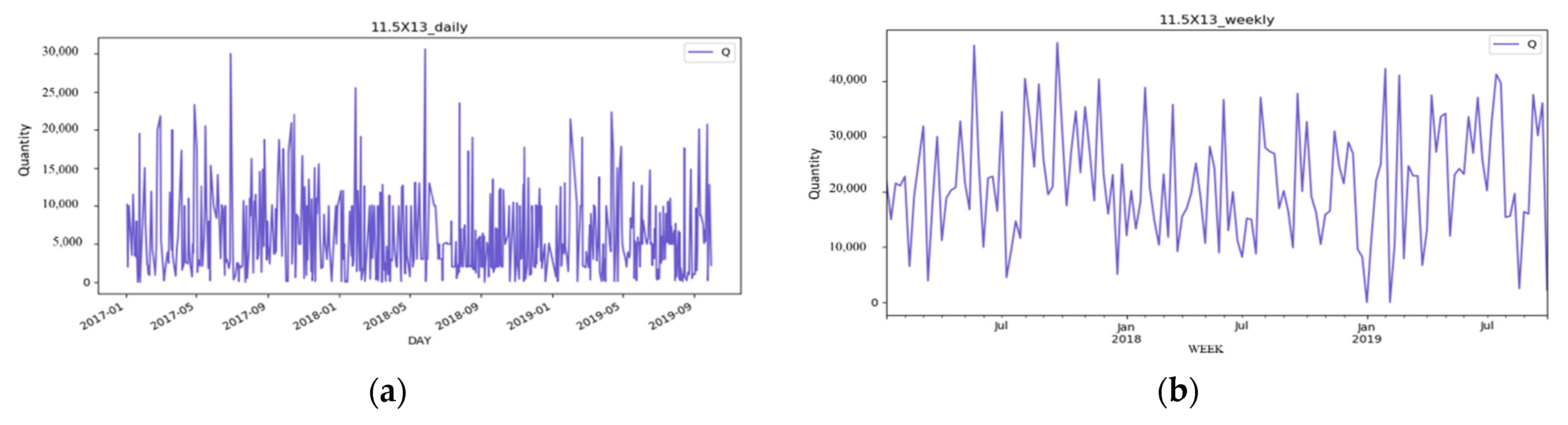
Based on the top three products offered by Industry–Academy Cooperation from 1 January 2017 to 29 September 2019, the proposed approach was validated. Time series are continuous data, and the approach of adding zeros is employed to deal with missing values in this study. The main reason is that, from a practical perspective, missing values show that no products were sold on that day, and the system does not record what caused the missing values. Since the case company calculates sales data every day, IC trays calculate material purchases every week. This study converts data measurement frequency from daily to weekly to forecast raw material demand. Figure 2 shows the BGA 11.5X13 product converted from daily to weekly units.

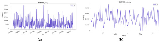
Figure 2. Timeline conversion of the difference graph. (a) BGA 11.5X13 timeline is daily; (b) BGA 11.5X13 timeline is one week.

2.2. Long Short-Term Memory Rolling Algorithm

Rolling forecasts are a type of dynamic forecasting. The main idea of this method is to add new data and delete old data simultaneously in a rolling manner while maintaining the length of the data. Forecasting results become more accurate through continuous learning, correction, and adjustment. The forecasting capability of an enterprise is thus enhanced so that it can respond promptly to customer needs [16]. Figure 3 illustrates a rolling forecasting process.

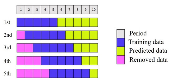
Figure 3. Rolling forecast schematic.

In 1997, Hochreiter proposed LSTM, a neural network model that solves the vanishing gradient problem for time series data [17]. LSTM regulates information flow, passes relevant information, and forecasts outcomes based on the incoming information. The previous hidden state is passed on to the next unit through the tanh activation function during the operation. A neural network’s hidden state acts as its memory, storing data it has seen in the past. A gate (forgetting, input, and output gates) allows the unit to decide whether to retain or delete information before passing it on to the next unit. Figure 4 shows the LSTM structure. The LSTM’s core, including input, output, and forgetting gates, is described below [18].

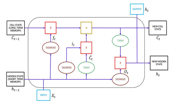
Figure 4. LSTM operational architecture.

• Forgetting gate: Based on the weights and the current input, the sigmoid function calculates a value $f_t$ between 0 and 1, determining which data will be retained and forgotten. Forgetting the data implies that they have been permanently removed from long-term memory. The forgetting gate’s equation is as follows:

  $$f_t=\sigma \left(W_f·\left[h_{t-1},X_t\right]+b_f\right)$$

  (1)

  where σ is the sigmoid function, ∙ is the dot product, $\left[h_{t-1},X_t\right]$ is a vector of input data, $W_f$ is the forgetting-gate weight, and $b_f$ is the forgetting-gate bias vector.
• Input gate: Given the weight, hidden state, and current input, the sigmoid function calculates $i_t$, a value between 0 and 1. This value is between 0 and 1, multiplied by the tanh activation function to calculate the cell status and determine which messages in long-term memory must be updated, including updated data and data that must be replaced to be employed in the future. The input gate’s equation is as follows

  $$i_t=\sigma \left(W_i·\left[h_{t-1},X_t\right]+b_i\right)$$

  (2)

  where $\sigma$ is the sigmoid function, $·$ is the dot product, $\left[h_{t-1}, X_t\right]$ is a vector of input data, $W_i$ is the input gate weight, and $b_i$ is the input gate bias vector.
  To update the long-term memory from $C_{t-1}$ at $t-1$ to $C_t$ at $t$, tanh computes the following equation, where $W_c$ is the tanh weight and $b_c$ is the tanh bias vector.

  $${\overline{C}}_t=tanh\left(W_c·\left[h_{t-1},X_t\right]+b_c\right)$$

  (3)
  If there are data that the forgetting gate and input gate wish to remove and add, respectively, the formula is as follows. First, to remove the forgetting gate’s data, $f_t\ast C_{t-1}$ is multiplied element by element, then the data that the input gate wishes to add are added element by element to update $I_t \ast {\overline{C}}_t$ to the long-term memory.

  $$C_t=f_t\ast C_{t-1}+I_t\ast {\overline{C}}_t$$

  (4)
• Output gate: According to the weight, hidden state, and current output, the sigmoid function computes $O_t$, which is between 0 and 1, and multiplies that value with the tanh activation function to determine which data should be removed from long-term memory $C_t$ to $t+1$ for further use. The output gate equation is as follows, where $\sigma$ is the sigmoid function, ∙ is the dot product operation, $\left[h_{t-1}, X_t\right]$ vector is the input data, $W_o$ is the output gate weight, and $b_O$ is the output gate bias vector.

  $$O_t=\sigma \left(W_o·\left[h_{t-1},X_t\right]+b_o\right)$$

  (5)
  In Figure 4, at the top right, $h_t$ are the output data sent to the output layer, and at the bottom, $h_t$ are the input data sent to $t+1$. The output data $h_t$ are obtained by multiplying the $C_t$ by the tanh activation function element by element after computing the output data $O_t$.

  $$h_t=O_t\ast \tanh \left(C_t\right)$$

  (6)

2.3. Individuals and Moving-Range (I-MR) Control Chart

Individual and moving-range charts comprise I and MR charts. I control charts are employed to demonstrate the means and variances of individual values, and MR control charts monitor the data’s variation. To effectively monitor all prediction processes, this study employs the I-MR control chart to determine whether error compensation is needed. If a point exceeds the control limits of the I-MR control chart, the error compensation mechanism is activated, and vice versa. The following are the steps to build an I-MR chart [19]:

Step 1.

Calculate the moving range (MR). The MR is calculated by calculating the distance between the 2 adjacent points.

$$M{R}_i=\left|x_i-x_{i-1}\right|$$

(7)

Step 2.

Calculate average $\left(\overline{x}\right)$ and Moving Range average $\left(\overline{MR}\right)$.

$$\overline{x}=\frac{{{\displaystyle \sum }}_{i=1}^k{x}_i}{k} , \overline{MR}=\frac{M{R}_i}{k-1}$$

(8)

where $x_i$ is the observed value of the i-th sample, k is the number of samples to establish the control chart.

Step 3.

Construct the control charts for the Individual and moving range.

$$\mathrm{Individual} \mathrm{control} \mathrm{chart}=\{\begin{array}{c}UCL=\overline{x}+3\frac{\overline{MR}}{d_2}\\ CL=\overline{x}\\ LCL=\overline{x}-3\frac{\overline{MR}}{d_2}\end{array}$$

(9)

$$\mathrm{Moving} \mathrm{range} \mathrm{control} \mathrm{chart}=\{\begin{array}{c}UCL=D_4\overline{MR}\\ CL=\overline{MR}\\ LCL=D_3\overline{MR}\end{array}$$

(10)

where, d₂, D₃, and D₄ are control chart constants [19].

It is important to remember that data that do not follow a normal distribution can affect the results when using I-MR control charts. Before using I-MR control charts, it is essential to check if the data are the normal distribution. It is recommended that the Box-Cox conversion method be used prior to plotting the I-MR chart if the data are not normally distributed.

2.4. Error Compensation Using ARMA Technique

It is difficult to develop an accurate model since the prediction error is uncertain [20]. The prediction results would be improved if an error compensation approach could be developed. More accurate prediction results can be obtained by compensating for the errors that are generated during training and combining them with the original prediction results [21].

Numerous scholars employ the ARMA model, which consists of autoregressive (AR) and moving average (MA), as an approach for error compensation, since it can determine the time series trend and predict future results. To study the evaporation process of alumina, Qian proposed particle-swarm optimization and ARMA error compensation [22]. Furthermore, microelectromechanical system gyroscopes are extensively employed in dynamic measurement devices. However, their measurement accuracy cannot be very accurate due to the external environment’s influence. Chen and Gao used the ARMA model for compensation to enhance the measurement accuracy of microelectromechanical system gyroscopes, which resulted in a 3.75% reduction in the measurement error [23].

In this study, the LSTM model was first developed. Then, the ARMA compensation model was developed by filtering the rolling prediction results by selected indicators (maximum, minimum, median, average, and the recent predicted results) and calculating the error from the actual values. This study employed the ARMA model since it does not need differencing, and the prediction results were corrected using the compensation values that were predicted by the ARMA model. The ARMA formula is as follows.

$$y_t=+{{\displaystyle \sum }}_{i=1}^p{\phi }_i{y}_{t-i}+{\epsilon }_t+{{\displaystyle \sum }}_{i=1}^q{\theta }_i{\epsilon }_{t-i}$$

(11)

where $y_t$ is the time series observation at time t; α is the constant; ${\phi }_i$ is the parameter of $y_{t-i}$ when the lag time is i; ${\epsilon }_t$ is the white noise at time t; p is the maximum lag-time step; ${\epsilon }_{t-i}$ is the white noise when the lag-time step is i; ${\theta }_i$ is the constant of ${\epsilon }_{t-i}$ when the lag-time step is i; q is the maximum lag-time step; and ARMA (p,q) is the ARMA model with the maximum lag-time step of the self-regression term p and the maximum lag-time step of the MA term q.

In constructing an ARMA model, the first step is to visualize the data and determine whether there are missing values. If there are missing values, this study will employ the zero-completion approach. Thereafter, the ARMA model’s parameters (p,q) are estimated, and the combination of parameters is obtained from the autocorrelation and partial autocorrelation functions., Along with the model, this is validated to determine whether the fitted model’s residual series is white noise. In the residual sequence, white noise is checked and the Akaike Information Criterion is employed to compute different levels and select the (p,q) combination with the lowest akaike information criterion (AIC) value. Finally, (p,q) is substituted into the ARMA model for prediction. Based on the error compensation, the prediction steps are as follows:

Step 1.

Calculate the mean absolute percentage error (MAPE), mean absolute error (MAE), and root mean squared error (RMSE) of each indicator, and select the one with the lowest error rate from the LSTM model.

Step 2.

Determine whether compensation is required by calculating the indicators’ errors and plotting the I-MR control chart.

Step 3.

In rolling LSTM, the number of products are predicted and multiple predictions are obtained for the test set.

Step 4.

The prediction result is filtered to $y_i^{\prime }$ based on the index that is selected in Step 1.

Step 5.

If compensation is needed, develop a rolling ARMA compensation model and calculate the compensation value $A_i$.

Step 6.

To obtain the compensation result $y_i^{\prime }$, add the compensation value $A_i$ to the filtered prediction result $y_i^{\prime \prime }$:

$$y_i^{″}=A_i+y_i^{\prime }.$$

(12)

Step 7.

Calculate the error $E_i$ between the actual value $y$ and $y_i^{″}$, i.e., $E_i=y_i^{″}-y$, which are the data for the next compensation model.

2.5. Data Partitioning and Parameter Setting

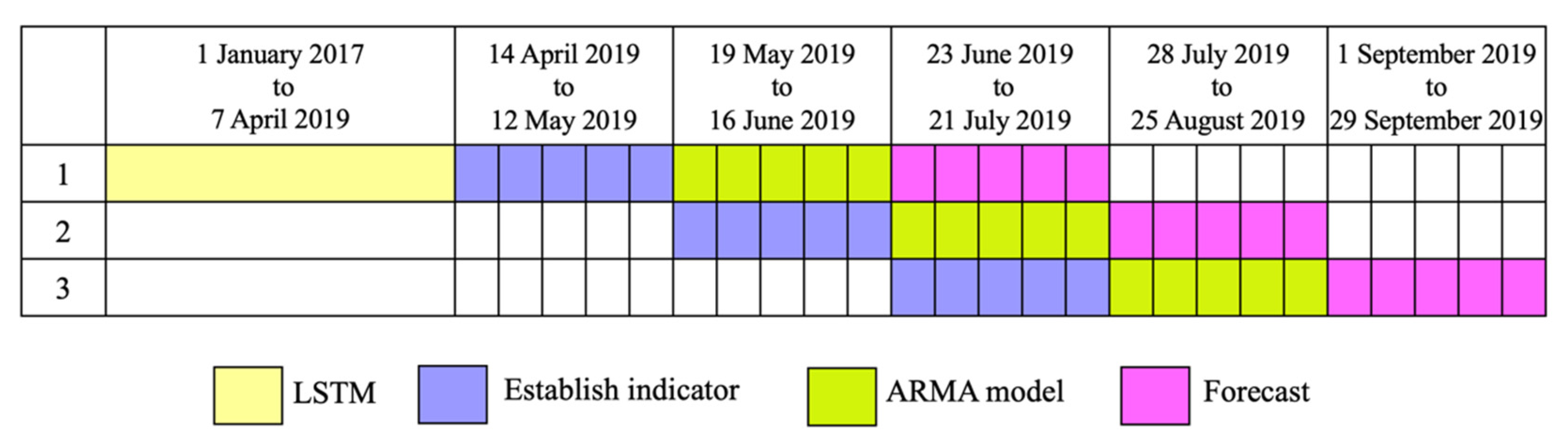
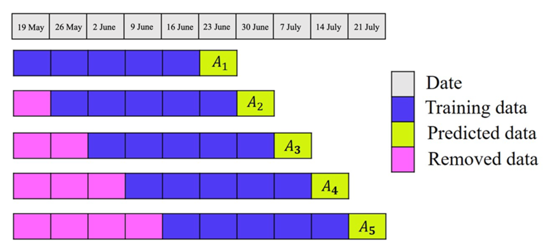
Figure 5 shows the rolling prediction process. As a first rollup, the data were divided into 118 weeks of yellow data from 1 January 2017 to 7 April 2019, five weeks of purple data from 14 April 2019 to 12 May 2019, and five weeks of green data from 19 May 2019 to 16 June 2019 for LSTM model training, indicators establishment, and compensation model building, respectively. Forecasting was based on pink section data from 23 June 2019 to 21 July 2019. The second rollup is based on the first compensation model values (19 May 2019–16 June 2019), a compensation model that was built using the first prediction (23 June 2019–21 July 2019), and a prediction of the last five data (28 July 2019–25 August 2019). This third rollup consists of an indicator that was constructed using the values from the second compensation model 23 June 2019–21 July 2019) and an indicator to the compensation model’s construction using the results from the second prediction (23 June 2019–21 July 2019). The third rollup uses the second compensation model (23 June 2019–21 July 2019), the second forecast (28 July 2019–25 August 2019) and predicts the last five data (1 September 2019–29 September 2019), and so on. In this study, only three cuts and rolls were made to the data to test the proposed approach.

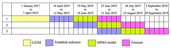
Figure 5. The rolling prediction process.

After the training samples are calculated, Table 1 shows the estimated LSTM rolling pattern parameters.

Table 1. LSTM parameter setting.

Parameter	Setting Values
Time step	1
Batch size	1
Loss function	MSE
Activation function	Sigmoid
Neurons	1
Hidden layers	4
Epochs	100
Optimizer	Adam

2.6. Model Performance Indicator

Different indicators are used to evaluate a model’s predictive power. Leonardo designed a forecasting model for sugarcane yield and compared the root mean squared error, mean absolute error, and mean absolute percentage error as indicators of the model’s predictive ability [24]. To predict the number of COVID-19 confirmations in Iran, Nasrin et al., developed a predictive model and evaluated the model’s performance using RMSE and MAE. The findings show that Iran was probably the most affected and needed more preventative measures [25]. Chang et al., developed a prediction model for air pollution and evaluated the model’s performance using the MAE, RMSE, and MAPE. The findings indicated that the model considerably enhanced the prediction’s accuracy [26]. MAE, RMSE, and MAPE, commonly used evaluation indicators in practice, are employed in this study as the criteria for model evaluation. This formula is defined as follows. When the index calculation result is small, predictability is better.

• MAE: The mean absolute error between the predicted $\widehat{y_t}$ and actual values $y_t$ of each datum is measured using the following formula:

  $$\mathrm{MAE}=\frac{1}{k}{\displaystyle {{\displaystyle \sum }}_{t=1}^k}\left|y_t-\widehat{y_t}\right|$$

  (13)
• RMSE: A measure of prediction error ($y_t-\widehat{y_t}$) standard deviation. The formula is as follows:

  $$\mathrm{RMSE}=\sqrt{\frac{1}{k}{\displaystyle {{\displaystyle \sum }}_{t=1}^k}{\left(y_t-\widehat{y_t}\right)}^2}$$

  (14)
• MAPE: This model overcomes the limitations of both mean absolute deviation (MAD) and RMSE using the relative prediction error of each data, which has overly large calculation results due to the large value of each data.

  $$\mathrm{MAPE}=\frac{1}{k}{\displaystyle {{\displaystyle \sum }}_{t=1}^k}\frac{\left|y_t-\widehat{y_t}\right|}{y_t}\times 100\%$$

  (15)
  $y_t$ is the actual value, $\widehat{y_t}$ is the predicted value, and k is the sample size. Mean square error (MSE) and MAPE are unaffected by unit and value sizes and are evaluated objectively; the larger the sample size, the higher the RMSE.

3. Analysis Results

A validation of the proposed methodology is provided in Section 3.1, Section 3.2 and Section 3.3 by analyzing and discussing the top three sales volumes of the product (BGA 11.5X13, BGA 8X13 and BGA 8X12.5).

3.1. Case Study of BGA 11.5X13

First, we employ rolling training with a fixed prediction window size, followed by initial training after every prediction. The initial training value is deleted upon each prediction and a new piece of data is added to the model. This is repeated until the specified period’s data have been predicted. The LSTM rolling model is employed for the 14 April 2019 to 12 May 2019 results, then the numerical results are computed based on maximum (Max), minimum (Min), median (Med), mean (Mean), and recent results (New), which are more commonly employed in statistics, and the values are filtered, as shown in Table 2.

Table 2. BGA 11.5X13 error calculation results of each indicator.

Date	14 April 2019	21 April 2019	28 April 2019	5 May 2019	12 May 2019
Actual value	37,500	27,200	33,600	34,200	12,000
Forecasting values	37,508	27,294	33,735	34,324	11,725
		27,289	33,681	34,264	11,829
			33,633	34,226	11,758
				34,397	11,791
					11,839
Max	37,508	27,294	33,735	34,397	11,839
Min	37,508	27,289	33,633	34,226	11,725
Med	37,508	27,291	33,681	34,294	11,791
Mean	37,508	27,291	33,683	34,303	11,789
New	37,508	27,289	33,633	34,397	11,839

RMSE, MAPE, and MAE were computed for each indicator, and the lowest error indicator was selected. For inconsistent results, as shown in Table 3, the median was selected as the indicator after RMSE calculation, the minimum after MAPE calculation, and the indicator with the most evaluated indicators was selected as the final decision, thus, the minimum (Min) will be selected as the next screening value.

Table 3. BGA 11.5X13 1st indicator calculation.

Indicator	RMSE	MAPE	MAE
Max	135.2800	1.6083	119
Min	130.7716	0.9780	86
Med	116.0070	1.2183	96
Mean	118.7021	1.2539	99
New	121.2253	1.2856	97

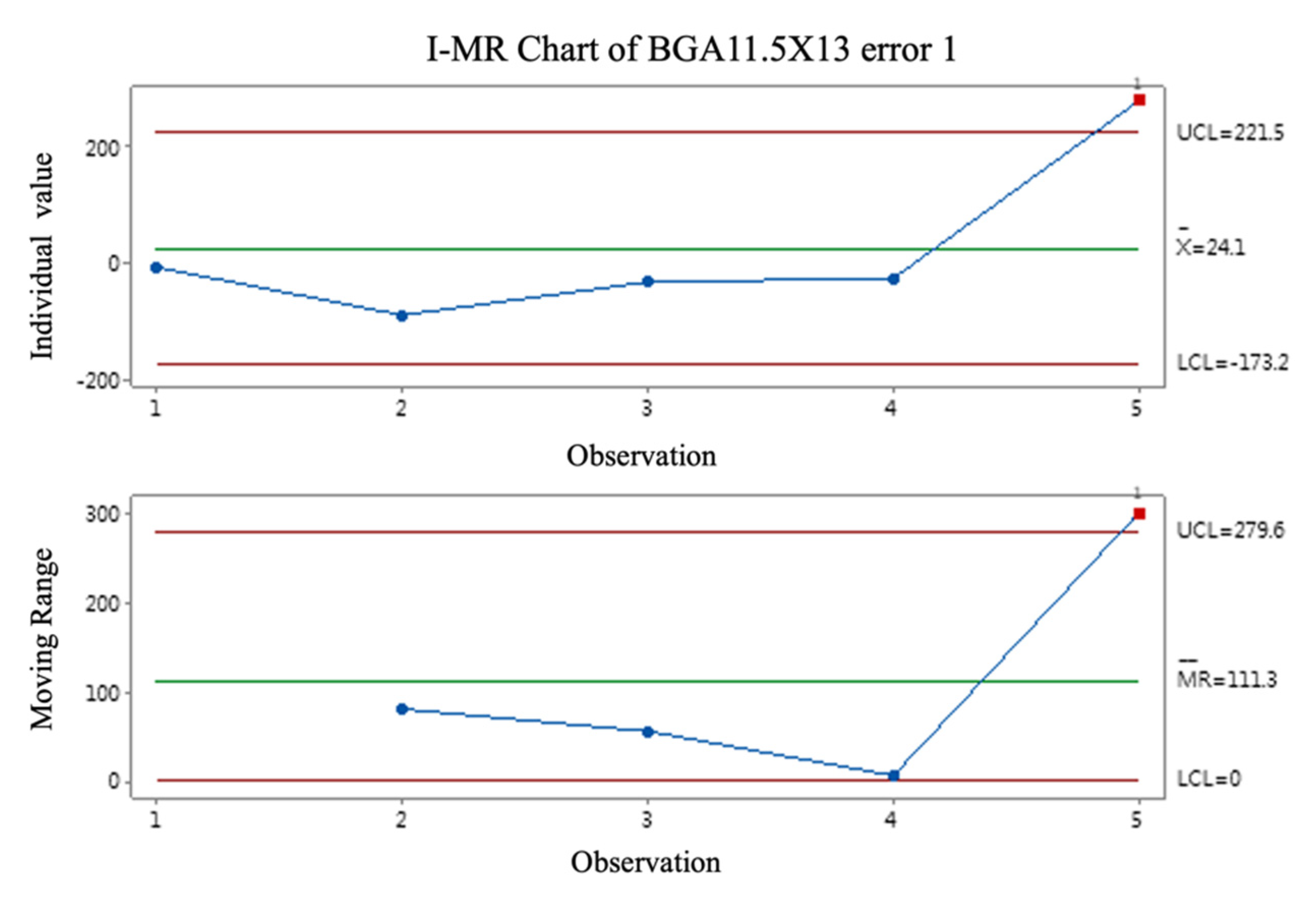
In Figure 6, the five errors in the selected metrics’ minimum values are plotted on the I-MR control chart, and if there are phenomena that exceed the control limits, the subsequent prediction results will be compensated.

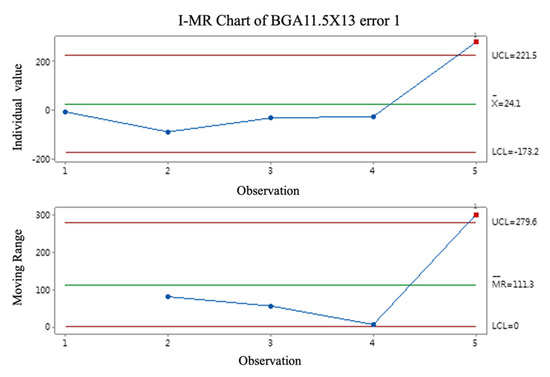
Figure 6. I-MR control chart for BGA 11.5X13 data for the first prediction roll.

As there is a condition of exceeding the control limits, an error compensation is required. Thereafter, the error is substituted into the ARMA model to obtain the compensation value $A_1$. To obtain the compensation result $y_1^{″}$, the compensation value $A_1$ is then summed with the prediction results after 23 June numerical screening. According to a previous rolling concept, the first 19 May error result is deleted, and a new 23 June error result is added. The new error is introduced in the compensation model from the result $y_1^{‴}$ resulting from the 23 June compensation and the actual error $E_1$. Then, the compensation value $A_2$ is compensated to the selected prediction of 30 June at the end of the week from 23 June to 21 July. Figure 7 shows a schematic representation of rolling error compensation.

Figure 7. Schematic representation of rolling error compensation.

A rolling LSTM was used for the prediction’s last five weeks, and the selected indicators’ values filtered the results, and Table 4 shows the calculated compensation values. The ARMA (p,q) value in Table 4 is (0,0) since this series is stationary, and ARMA is the most extensively employed model for fitting stationary series.

Table 4. The result of calculating compensation value at different time points.

Date	ARMA (p,q)	Compensation
23 June 2019	ARMA (0,0)	307
30 June 2019	ARMA (0,0)	203
7 July 2019	ARMA (0,0)	141
14 July 2019	ARMA (0,0)	79
21 July 2019	ARMA (0,0)	40

Table 5 summarizes the three rolling prediction results, in which the errors are computed by subtracting the actual values from the predicted values. In Table 5, the rolling prediction’s error with indicator filtering (LSTM-Min) is smaller than the LSTM prediction. If the previous judgment requires error compensation (LSTM-ARMA), the error remains smaller than in the previous two approaches.

Table 5. BGA 11.5X13 rolling forecast results summary.

1	Date	Actual Value	LSTM	Error	LSTM-Min	Error	LSTM-ARMA	Error
	23 June	37,100	36,894	−206	36,934	−166	37,141	41
	30 June	25,800	25,437	−363	25,567	−233	25,791	−9
	7 July	20,200	19,708	−492	19,999	−201	20,157	−43
	14 July	32,600	32,476	−124	32,523	−77	32,614	14
	21 July	41,300	41,136	−164	41,176	−124	41,227	−73
2	Date	Actual value	LSTM	Error	LSTM-Min	Error	LSTM-ARMA	Error
	28 July	39,700	39,941	241	39,491	−209	39,571	−129
	4 August	15,400	15,492	92	15,325	−75	15,399	−1
	11 August	15,600	15,764	164	15,572	−28	15,616	16
	18 August	19,700	19,760	60	19,648	−52	19,674	−26
	25 August	2500	2661	161	2452	−48	2488	−12
3	Date	Actual value	LSTM	Error	LSTM-Min	Error	LSTM-ARMA	Error
	1 September	16,400	16,352	−48	16,378	−22	16,412	12
	8 September	16,000	16,352	352	16,219	219	16,209	209
	15 September	37,600	37,480	−120	37,706	106	37,653	53
	22 September	30,200	30,037	−163	30346	146	30,300	100
	29 September	36,100	36,309	209	36,246	146	36,199	99

3.2. Case Study of BGA 8X13

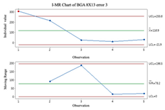
Table 6 summarizes the results of the BGA 8X13’s three rolls, showing that the median was selected as the filtering indicator, and since the I-MR control chart did not exceed the control limits, no error correction was necessary. The mean was selected as the filtering indicator for the second roll, and no error compensation was required since the I-MR control chart did not exceed the control limits. The median was selected as the filtering indicator in the third roll, and since the I-MR control chart did not exceed the control limits, an error compensation was necessary. In the third rollover, the median was selected as the filter and the I-MR control chart exceeded the control limits, so error correction was necessary.

Table 6. BGA 8X13 three rolling results.

	1	2	3
Indicator	Med	Mean	Min
I-MR control chart
Error compensation	Not required	Not required	Required

Table 7 summarizes the three rolling prediction results by subtracting the actual values from the predicted values and by calculating the errors. In Table 7, the rolling prediction’s error combined with the indicator filtering approach is smaller than the general LSTM prediction’s error. If the previous judgment requires error compensation, the error after compensation is smaller than the previous two approaches’ errors.

Table 7. BGA 8X13 rolling forecast results summary.

1	Date	Actual Value	LSTM	Error	LSTM-Med	Error	LSTM-ARMA	Error
	23 June	36,900	36,395	−505	36,595	−305
	30 June	40,700	40,487	−213	40,576	−124
	7 July	50,100	50,074	−26	50,117	17
	14 July	59,000	58,989	−11	58,987	−13
	21 July	49,800	49,770	−30	49,914	114
2	Date	Actual value	LSTM	Error	LSTM-Mean	Error	LSTM-ARMA	Error
	28 July	16,000	15,978	−22	15,988	−12
	4 August	23,400	23,321	−79	23,335	−65
	11 August	69,200	69,024	−176	69,302	102
	18 August	36,700	36,793	93	36,752	52
	25 August	31,900	31,931	31	31,863	−37
3	Date	Actual value	LSTM	Error	LSTM-Min	Error	LSTM-ARMA	Error
	1 September	73,800	73,638	−162	73,758	−42	74,011	211
	8 September	51,200	51,287	87	51,020	−180	51,269	69
	15 September	45,800	46,169	369	45,457	−343	45,602	−198
	22 September	49,600	49,959	359	49,371	−229	49,520	−80
	29 September	29,500	29,476	−24	29,269	−231	29,385	−115

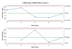
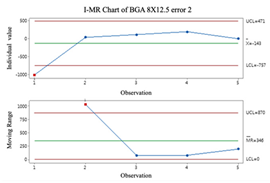
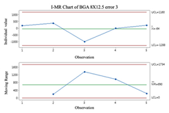
3.3. Case Study of BGA 8X12.5

Table 8 summarizes the three BGA 8X12.5 rollover results. It shows that the first rollover selects the maximum value as the numerical filter, and the I-MR control chart does not exceed the control limits; therefore, no error compensation is necessary. In the second rollover, the median is selected as the numerical filter, and the I-MR control chart does not exceed the control limits, thus, error compensation is necessary. In the third rollover, the nearest result is the numerical filter, and error compensation is not required if the I-MR control chart does not exceed the control limits.

Table 8. BGA 8X12.5 three rolling results.

	1	2	3
Indicator	Max	Med	New
I-MR control chart
Error compensation	Not required	Required	Not required

Table 9 summarizes the results of the three rolling predictions, where the error is calculated by subtracting the actual values from the predicted values. In Table 9, the rolling prediction combined with the indicator filter is more accurate than the general LSTM prediction; if the previous judgment requires error compensation, the error after compensation is smaller than that of the previous two approaches.

Table 9. BGA 8X12.5 rolling forecast results summary.

1	Date	Actual Value	LSTM	Error	LSTM-Max	Error	LSTM-ARMA	Error
	23 June	20,900	20,735	−165	20,935	35
	30 June	22,500	22,334	−166	22,634	134
	7 July	1400	1439	39	1445	45
	14 July	32,400	32,405	5	32,517	117
	21 July	13,600	13,579	−21	13,704	104
2	Date	Actual value	LSTM	Error	LSTM-Med	Error	LSTM-ARMA	Error
	28 July	10,900	11,014	114	11,004	104	10,916	16
	4 August	10,800	10,999	199	10,986	186	10,864	64
	11 August	21,400	21,529	129	21,529	129	21,340	−60
	18 August	11,700	11,663	−37	11,669	−31	11,712	12
	25 August	23,900	23,835	−65	23,858	−42	23,877	−23
3	Date	Actual value	LSTM	Error	LSTM-New	Error	LSTM-ARMA	Error
	1 September	31,400	31,412	12	31,422	22
	8 September	100	366	266	268	168
	15 September	11,300	11,212	−88	11,341	41
	22 September	23,200	22,924	−276	23,310	110

3.4. Model Evaluation

These three cases study are compared for the traditional LSTM approach, the rolling LSTM prediction using the indicator filtering numerical approach, and the LSTM-ARMA compensation approach. Table 10 shows the evaluation results using the RMSE, the MAPE, and the MAE.

Table 10. Comparison of RMSE, MAPE, and MAE results for three different IC trays.

IC Trays Code		RMSE			MAPE			MAE
		LSTM	LSTM-Index	LSTM-ARMA	LSTM	LSTM-Index	LSTM-ARMA	LSTM	LSTM-Index	LSTM-ARMA
BGA 11.5X13	1	302.830	169.336	42.746	1.035	0.576	0.116	269.8	160.2	36.0
	2	156.820	105.092	59.385	1.800	0.676	0.206	143.6	82.4	36.8
	3	205.357	143.006	115.360	0.786	0.535	0.426	178.4	127.8	94.7
BGA 8X13	1	245.801	156.112	NA	0.405	0.283	NA	157.0	114.6	NA
	2	97.274	61.298	NA	0.216	0.151	NA	80.2	53.5	NA
	3	244.717	226.987	147.045	0.400	0.480	0.281	200.2	205.0	134.6
BGA 8X12.5	1	106.553	95.615	NA	0.897	1.021	NA	79.2	87.0	NA
	2	122.337	113.823	41.533	0.816	0.744	0.244	108.8	98.4	35.0
	3	194.636	110.687	NA	53.772	33.907	NA	165.6	95.6	NA

Notes: NA stated that it is not necessary to activate the compensation mechanism.

There is a decreasing trend in terms of the RMSE; however, the rolling LSTM prediction combined with pointer screening offers a better prediction result than LSTM. If error compensation is required, the LSTM-ARMA approach results indicate a significant decrease in RMSE compared with the aforementioned approaches. In terms of MAPE, there is a decreasing trend, however, in most cases, the rolling LSTM prediction combined with the screening of indicators presents a better prediction result than the LSTM, probably because the demand for the case company’s orders is more volatile and the model cannot be more accurate. The MAE trend is declining, but most of the rolling LSTM prediction combined with indicator filtering offers better predictions than the LSTM, perhaps because demands for the company’s orders are more volatile, and the model cannot predict more accurately. If the error compensation is required, the MAE of LSTM-ARMA tends to decrease compared with the aforementioned approaches.

4. Discussion and Conclusions

The prediction model results’ accuracy improved due to the demand of competitors in the market. The forecasting model that is developed in this study is based on actual data from the case companies and is compared with the way that it was previously used. This study had three primary findings. At one time, forecasts were performed for one point at a time, i.e., tomorrow’s results were predicted as they would be. We forecast five points at a time, i.e., tomorrow, the day after tomorrow, the day after tomorrow, the day after tomorrow, etc. In the case of a later forecast, there is not only one forecast, but also the findings from the current period, the previous period, and the previous period before that. Several values are filtered using indicators, instead of using the most recent result as the final forecast. Second, in the past, we would pause the model and reload the data for new model training if we encountered poor prediction results, but this process was tedious and complicated. Finally, in the past, error compensation was activated regardless of the prediction results. The proposed error compensation mechanism is based on the I-MR control chart that is plotted by the difference between the indicators’ filtered and actual values, and the need for error compensation is determined as opposed to simply activating compensation regardless of the prediction results.

LSTM, rolling LSTM combined with an index, and LSTM-ARMA are compared, and the LSTM-ARMA approach proves to be more accurate when the error compensation is required. Furthermore, the rolling LSTM combined with the index offers better predictions than the firm’s rule of thumb and LSTM when no residential error compensation is required. Table 11 shows the evaluation of the ARIMA model, demonstrating that the LSTM-ARMA method is more accurate when error compensation is required.

Table 11. Results of the comparison between traditional ARIMA and our proposed LSTM-ARMA for three IC trays.

IC Trays Code		ARIMA			LSTM-ARMA (In This Paper)
		RMSE	MAPE	MAE	RMSE	MAPE	MAE
BGA 11.5X13	1	3507.883	0.341	301.8	42.746	0.116	36.0
	2	3707.6	0.21	241.5	59.385	0.206	36.8
	3	424.53	0.53	180.4	115.360	0.426	94.7
BGA 8X13	1	9108.204	28.3	160.2	NA	NA	NA
	2	9332.74	26.2	50.2	NA	NA	NA
	3	9441.83	19.8	297.2	147.045	0.281	134.6
BGA 8X12.5	1	1061.469	31.21	470.2	NA	NA	NA
	2	1204.73	32.63	68.8	41.533	0.244	35.0
	3	1509.21	33.97	265.6	NA	NA	NA

Notes: NA stated that it is not necessary to activate the compensation mechanism.

As a contribution to academic work, we have proposed an approach to determine whether an error compensation is necessary using rolling data for forecasting. In cases of model inaccuracy, the original model can be used without model correction. Combining LSTM and ARMA rolling forecasting approaches can generate more accurate forecasting results and eliminate the bottleneck problems that have been experienced in the past. In the past, regarding industry contribution, models were trained and tested before going online, and once they were employed, they gradually became inaccurate and needed to be recorrected, which took a long time. This study develops a model that uses error compensation to reduce the time and cost of pausing the model correction when past forecasts are inaccurate and compares it with empirical rules that are employed by companies to offer more accurate forecasting results.

References

- Guo, D.Y.; Shi, H.Z.; Qian, Y.P.; Lv, M.; Li, P.G.; Su, Y.L.; Tang, W.H. Fabrication of β-Ga2O3/ZnO heterojunction for solar-blind deep ultraviolet photodetection. Semicond. Sci. Technol. 2017, 32, 03LT01. [Google Scholar] [CrossRef]
- Kumar, V.; Dwivedi, S.K. Hexavalent chromium stress response, reduction capability and bioremediation potential of Trichoderma sp. isolated from electroplating wastewater. Ecotoxicol. Environ. Saf. 2019, 185, 109734. [Google Scholar] [CrossRef]
- Wang, C.-C.; Chien, C.-H.; Trappey, A.J.C. On the Application of ARIMA and LSTM to Predict Order Demand Based on Short Lead Time and On-Time Delivery Requirements. Processes 2021, 9, 1157. [Google Scholar] [CrossRef]
- Aparna, S. Long Short-Term Memory and Rolling Window Technique for Modeling Power Demand Prediction. In Proceedings of the International Conference on Intelligent Computing and Control Systems, Madurai, India, 14–15 June 2018; pp. 1675–1678. [Google Scholar]
- Park, S.; Lehto, X.; Lehto, M. Self-service technology kiosk design for restaurants: An QFD application. Int. J. Hosp. Manag. 2020, 92, 102757. [Google Scholar] [CrossRef]
- Bi, J.-W.; Li, H.; Fan, Z.-P. Tourism demand forecasting with time series imaging: A deep learning model. Ann. Tour. Res. 2021, 90, 103255. [Google Scholar] [CrossRef]
- Tanizaki, T.; Hoshino, T.; Shimmura, T.; Takenaka, T. Demand forecasting in restaurants using machine learning and statistical analysis. Procedia CIRP 2019, 79, 679–683. [Google Scholar] [CrossRef]
- Liu, W.; Liu, W.D.; Gu, J. Forecasting oil production using ensemble empirical model decomposition based Long Short-Term Memory neural network. J. Pet. Sci. Eng. 2020, 189, 107013. [Google Scholar] [CrossRef]
- Yu, P.; Yan, X. Stock price prediction based on deep neural networks. Neural Comput. Appl. 2019, 32, 1609–1628. [Google Scholar] [CrossRef]
- Mayr, J.; Blaser, P.; Ryser, A.; Hernández-Becerro, P. An adaptive self-learning compensation approach for thermal errors on 5-axis machine tools handling an arbitrary set of sample rates. CIRP Ann. 2018, 67, 551–554. [Google Scholar] [CrossRef]
- Liang, X.; Zhang, S.; Wu, Y.; Xing, J.; He, X.; Zhang, K.M.; Wang, S.; Hao, J. Air quality and health benefits from fleet electrification in China. Nat. Sustain. 2019, 2, 962–971. [Google Scholar] [CrossRef]
- Ma, J. Telework Triggered by Epidemic: Effective Communication Improvement of Telecommuting in Workgroups during COVID-19. Am. J. Ind. Bus. Manag. 2021, 11, 202. [Google Scholar] [CrossRef]
- Vagal, A.; Reeder, S.B.; Sodickson, D.K.; Goh, V.; Bhujwalla, Z.M.; Krupinski, E.A. The impact of the COVID-19 pandemic on the radiology research enterprise: Radiology scientific expert panel. Radiology 2020, 296, E134–E140. [Google Scholar] [CrossRef] [PubMed] [Green Version]
- Jiang, J.; Marsh, T.L.; Tozer, P.R. Policy induced price volatility transmission: Linking the US crude oil, corn and plastics markets. Energy Econ. 2015, 52, 217–227. [Google Scholar] [CrossRef]
- Hu, C.; Liu, X.; Pan, B.; Chen, B.; Xia, X. Asymmetric impact of oil price shock on stock market in China: A combination analysis based on SVAR model and NARDL model. Emerg. Mark. Financ. Trade 2017, 54, 1693–1705. [Google Scholar] [CrossRef]
- O’Connor, M.; Remus, W.; Griggs, K. Does updating judgmental forecasts improve forecast accuracy? Int. J. Forecast. 2000, 16, 101–109. [Google Scholar] [CrossRef]
- Hochreiter, S.; Schmidhuber, J. Long short-term memory. Neural Comput. 1997, 9, 1735–1780. [Google Scholar] [CrossRef]
- Abbasimehr, H.; Shabani, M.; Yousefi, M. An optimized model using LSTM network for demand forecasting. Comput. Ind. Eng. 2020, 143, 106435. [Google Scholar] [CrossRef]
- Montgomery, D.C. Introduction to Statistical Quality Control; John Wiley & Sons: New York, NY, USA, 2009. [Google Scholar]
- He, X.; Deng, K.; Wang, X.; Li, Y.; Zhang, Y.; Wang, M. Lightgcn: Simplifying and powering graph convolution network for recommendation. In Proceedings of the 43rd International ACM SIGIR conference on research and development in Information Retrieval, Xi’an, China, 25–30 July 2020; pp. 639–648. [Google Scholar]
- Liang, C.-J.; Liang, J.-J.; Jheng, C.-W.; Tsai, M.-C. A rolling forecast approach for next six-hour air quality index track. Ecol. Inform. 2020, 60, 101153. [Google Scholar] [CrossRef]
- Qian, X. Parameter prediction based on Improved Process neural network and ARMA error compensation in Evaporation Process. In IOP Conference Series: Earth and Environmental Science; IOP Publishing: Bristol, UK, 2018; Volume 108, p. 022078. [Google Scholar]
- Chen, M.M.; Gao, G.W. Research on MEMS gyroscope random error compensation algorithm based on ARMA model. Appl. Mech. Mater. 2014, 602, 891–894. [Google Scholar] [CrossRef]
- Maldaner, L.F.; de Paula Corrêdo, L.; Canata, T.F.; Molin, J.P. Predicting the sugarcane yield in real-time by harvester engine parameters and machine learning approaches. Comput. Electron. Agric. 2021, 181, 105945. [Google Scholar] [CrossRef]
- Talkhi, N.; Fatemi, N.A.; Ataei, Z.; Nooghabi, M.J. Modeling and forecasting number of confirmed and death caused COVID-19 in IRAN: A comparison of time series forecasting methods. Biomed. Signal Process. Control 2021, 66, 102494. [Google Scholar] [CrossRef] [PubMed]
- Chang, Y.S.; Chiao, H.T.; Abimannan, S.; Huang, Y.P.; Tsai, Y.T.; Lin, K.M. An LSTM-based aggregated model for air pollution forecasting. Atmos. Pollut. Res. 2020, 11, 1451–1463. [Google Scholar] [CrossRef]
Publisher’s Note: MDPI stays neutral with regard to jurisdictional claims in published maps and institutional affiliations. |
© 2022 by the authors. Licensee MDPI, Basel, Switzerland. This article is an open access article distributed under the terms and conditions of the Creative Commons Attribution (CC BY) license (https://creativecommons.org/licenses/by/4.0/).