Optimal Control with Partially Observed Regime Switching: Discounted and Average Payoffs

Abstract

We consider an optimal control problem with the discounted and average payoff. The reward rate (or cost rate) can be unbounded from above and below, and a Markovian switching stochastic differential equation gives the state variable dynamic. Markovian switching is represented by a hidden continuous-time Markov chain that can only be observed in Gaussian white noise. Our general aim is to give conditions for the existence of optimal Markov stationary controls. This fact generalizes the conditions that ensure the existence of optimal control policies for optimal control problems completely observed. We use standard dynamic programming techniques and the method of hidden Markov model filtering to achieve our goals. As applications of our results, we study the discounted linear quadratic regulator (LQR) problem, the ergodic LQR problem for the modeled quarter-car suspension, the average LQR problem for the modeled quarter-car suspension with damp, and an explicit application for an optimal pollution control.

1. Introduction

In recent years, there has been more attention to a class of optimal control problems where the dynamic systems are governed means switching diffusions in which the switching is modeled by a continuous-time Markov chain ($\psi$) with unobservable hidden states (also known as partially observed optimal control problems). In these problems, an observable process y whose outcomes are “influenced” by the outcomes of $\psi$ in a known way is assumed. Since $\psi$ cannot be observed directly, the goal is to learn about $\psi$ by observing y. Following the last mentioned, this article concerns with an optimal control problem with discounted and ergodic payoff in which the dynamic system $x\left(t\right)$ evolves according to a Markovian regime-switching diffusion $dx\left(t\right)=f\left(x\right(t),\psi (t\left)\right)dt+\sigma \left(x\right(t),\psi (t\left)\right)dW\left(t\right)$ for given continuous functions f and $\sigma$. The reward rate is allowed to be unbounded from above and from below. In this paper, the Wonham filter to estimate the states of the Markov chain from the observable evolution of a given process (y) is used. As a result, the original system $x\left(t\right)$ is converted to a completely observable one $\overline{x}\left(t\right)$.

Our main results extend the dynamic programming technique to this family of stochastic optimal control problems with reward (or cost) rate per unit of time unbounded and Markovian regime-switching diffusions. The regime switching is modeled by a continuous-time Markov chain ($\psi$) with unobservable states. Early works include research on an optimal control problem with an ergodic payoff, considering that the dynamic system evolves according to Markovian switching diffusions. However, this diffusion does not depend on a hidden Markov chain [1]. Research on deriving the dynamic programming principle for a partially observed optimal control problem in which the dynamic system is governed by a discrete-time Markov control process taking values in a finite-dimensional space has also been proposed [2]. Finally, one paper studied the optimal control with Markovian switching that is completely observable and rewards rate unbounded [3]. As an application of our results, we study the discounted linear quadratic regulator (LQR) problem, the ergodic LQR problem for the modeled quarter-car suspension, the average (ergodic) LQR problem for the modeled quarter-car suspension with damp, and an explicit application for an optimal pollution control. Other applications with bounded payoff different from those studied in this work are found in [4,5,6].

The objective of the theory of controlled regime-switching diffusions is to model controlled diffusion systems whose dynamics are affected by discrete phenomena. In these systems, the discrete phenomena are modeled by a Markov chain in continuous time, whose states represent the discrete phenomenon involved. There is an extensive list of references dealing with the case of completely observable stochastic optimal control in which a switching diffusion governs the stochastic systems. A literature review includes the textbooks [7,8] and the papers [9,10,11,12,13,14], with several applications, including optimization portfolios, wireless communication systems, and wind turbines, among others.

Generally, to solve unobserved optimal control problems, where the dynamic systems are governed by a hidden Markovian switching diffusion, it is necessary to transform them into completely observed ones, which in our case is done using a Wonham filter.

This Wonham filter estimates the hidden state of the Markov chain from the observable evolution of the process y. When these estimates are replaced in the original system, this becomes a completely observable system [15,16] and ([17], Section 22.3). The numerical results for Wonham’s filter are given in [18].

The paper is organized as follows: in Section 1, an introduction is given. In Section 2, the main assumptions are given. In this section, the partially observable system is converted into an observable system. The conditions to ensure the existence of optimal solutions for the optimal control problem with discounted payoff are given in Section 3. In Section 4, the conditions to ensure the existence of optimal solutions for the optimal control problem with average payoff are deduced. To illustrate our results, four applications are developed: an application on a linear quadratic regulator (LQR) with discounted payoff (Section 5); the development of a model of a quarter-car suspension LQR with an average payoff (Section 6); the study of an optimal control of a vehicle active suspension system with damp (Section 7); and an explicit application for an optimal pollution control (Section 8).

2. Formulation of the Problem

This work focuses on controlled hybrid stochastic differential Equations (HSDE) under partial observation. To explain this, first, we consider the stochastic differential equations of the form:

$$\mathrm{d}x\left(t\right)=b(x\left(t\right),\psi \left(t\right),u\left(t\right))\mathrm{d}t+\sigma (x\left(t\right),\psi \left(t\right))\mathrm{d}W\left(t\right),x\left(0\right)=x_0,\psi \left(0\right)=i,$$

(1)

where $b:{\mathbb{R}}^n\times E\times \mathcal{U}\to {\mathbb{R}}^n$ and $\sigma :{\mathbb{R}}^n\times E\to {\mathbb{R}}^{n\times d}$ in (1) depend on a finite state and time-continuous irreducible and aperiodic Markov chain $\psi (·)$ taking values in $E=\{1,\dots ,N\}$. For all $i,j\in E$ the transition probabilities are given by:

$$\begin{array}{c}\hfill \mathbb{P}\left(\psi \right(s+t\left)\right)=j\mid \psi \left(s\right)=i=& \left\{\begin{array}{cc}{q}_{ij}t+o\left(t\right),\hfill & \mathrm{if}i\ne j,\hfill \\ 1+q_{ii}t+o\left(t\right),\hfill \end{array}\right.\end{array}$$

where the constants $q_{ij}\ge 0$ are the transition rates from i to j and satisfy that $q_{ii}\left(x\right)=-{\sum }_{i\ne j}{q}_{ij}\left(x\right)$, the transition matrix is denoted by $Q={\left\{q_{ij}\right\}}_{i,j=1,2,\dots ,N}$. The control component is $u\left(t\right)\in \mathcal{U}$ with $\mathcal{U}$ a compact set of ${\mathbb{R}}^m$, and W is a d-dimensional standard Brownian motion independent of $\psi (·)$. Throughout the work, it is considered that both the Markov chain $\psi (·)$ and the Brownian motion W are defined on a complete filtered probability space $(\Omega ,\mathcal{F},\mathbb{P},\left\{{\mathcal{F}}_t\right\})$ that satisfies the usual conditions.

Until now, the switching diffusion (1) seems to be formulated as a classical switching diffusion, as in [11,12,13,14,19], among others. However, we propose that the process $\psi$ is a hidden Markov chain, i.e., at any given instant of time, the exact state of the Markov chain $\psi (·)$ cannot be observed directly. Instead, we can only observe the process y given by:

$$dy\left(t\right)=h\left(\psi \left(t\right)\right)\mathrm{d}t+{\sigma }_0\mathrm{d}B\left(t\right),y\left(0\right)=0,$$

(2)

whose dynamics depends on the value of $\psi (·)$. In Equation (2), $h:E\to \mathbb{R}$ is a bounded function, whereas B is a one-dimensional Brownian motion independent of W and $\psi$, and ${\sigma }_0$ is a positive constant.

Under partial observation, the best way to work is through nonlinear filtering. This technique studies the conditional distribution of $\psi \left(t\right)$ given the observed data accumulated up to time t, namely:

$$\begin{array}{c}\hfill {\Psi }_i\left(t\right)=\mathbb{P}(\psi \left(t\right)=i|{\sigma }_1(y\left(s\right),0\le s\le t)),\forall i\in E,\end{array}$$

(3)

where ${\sigma }_1(y\left(s\right),0\le s\le t))$ is the ${\sigma }_1$-algebra generated by the process $y\left(t\right)$ and ${\sum }_{i=1}^N{\Psi }_i\left(t\right)=1.$ Taking into account the following notation:

$$\begin{array}{cc}\hfill h^T(\Psi )& =\left(h\right(1),h(2),\dots ,h(N\left)\right),\hfill \\ \hfill {\Psi }^T\left(t\right)& =({\Psi }_1\left(t\right),\dots ,{\Psi }_N\left(t\right)),\hfill \\ \hfill \mathrm{diag}\left(h\right)& =\mathrm{diag}\left(h\right(1),\dots ,h(N\left)\right),\hfill \end{array}$$

and using the Wonham filtering techniques, we know that the process $\Psi$ in (3) satisfies the following Equation (see for instance [15] or ([17], Section 22.3)):

$$\begin{array}{cc}\hfill \mathrm{d}\Psi \left(t\right)=& \left[Q\Psi \left(t\right)-{\sigma }_0^{-2}{h}^T(\Psi \left(t\right))\left(\mathrm{diag}\left(h\right)-h^T(\Psi \left(t\right))I_N\right)\Psi \left(t\right)\right]\mathrm{d}t\hfill \\ \hfill +& {\sigma }_0^{-2}\left(\mathrm{diag}\left(h\right)-h^T(\Psi \left(t\right))I_N\right)\Psi \left(t\right)\mathrm{d}y\left(t\right),\hfill \end{array}$$

(4)

where $I_N$ is the $N\times N$ identity matrix. If we introduce the process:

$$\mathrm{d}{w}_0\left(t\right)={\sigma }_0^{-1}(\mathrm{d}y\left(t\right)-h^T(\Psi \left(t\right))dt),$$

then Equation (4) can be rewritten as:

$$\begin{array}{c}\hfill \mathrm{d}\Psi \left(t\right)=Q\Psi \left(t\right)\mathrm{d}t+{\sigma }_0^{-1}\left(\mathrm{diag}\left(h\right)-h^T(\Psi \left(t\right))I_N\right)\Psi \left(t\right)\mathrm{d}{w}_0\left(t\right).\end{array}$$

(5)

Remark 1.

Note that the unique solution of (5) exists up to an explosion time τ (see, for instance [20]). However, $\tau =\infty$ a.s. since ${\Psi }_i\left(t\right)\le 1$ for all $t<\tau$ and $\forall i\in E$.

At this point, we have defined the controlled HSDE with partial observation. To fulfill the objective of this work, that is, to solve an optimal control problem with the discounted and average payoff with partial observation, we will transform this problem into one with complete observation (see for instance [5,6,16]). First, we will establish the following notational convention.

For the coefficients $b:{\mathbb{R}}^n\times E\times \mathcal{U}\to {\mathbb{R}}^n$ and $\sigma :{\mathbb{R}}^n\times E\to {\mathbb{R}}^{n\times d}$

$$\begin{array}{cc}\hfill b\left(x\right(t),\psi (t),u(t\left)\right)& =(b_1(x\left(t\right),\psi \left(t\right),u\left(t\right)),\dots ,b_n(x\left(t\right),\psi \left(t\right),u\left(t\right))),\hfill \\ \hfill \sigma \left(x\right(t),\psi (t\left)\right)& ={\left\{{\sigma }_{kl}(x\left(t\right),\psi \left(t\right))\right\}}_{k=1,\dots ,n;l=1,\dots ,d},\hfill \end{array}$$

we have their filtered estimates:

$$\begin{array}{cc}\hfill {\overline{b}}_k(x\left(t\right),\Psi \left(t\right),u\left(t\right))& =\sum _{i=1}^N{\Psi }_i\left(t\right)b_k(x\left(t\right),i,u\left(t\right)),\hfill \end{array}$$

(6)

$$\begin{array}{cc}\hfill {\overline{\sigma }}_{kl}(x\left(t\right),\Psi \left(t\right))& =\sum _{i=1}^N{\Psi }_i\left(t\right){\sigma }_{kl}(x\left(t\right),i),\hfill \end{array}$$

(7)

and with equalities (6)–(7), we establish the new coefficients:

$$\begin{array}{cc}\hfill \overline{b}(x\left(t\right),\Psi \left(t\right),u\left(t\right))& =({\overline{b}}_1(x\left(t\right),\Psi \left(t\right),u\left(t\right)),\dots ,{\overline{b}}_n(x\left(t\right),\Psi \left(t\right),u\left(t\right))),\hfill \\ \hfill \overline{\sigma }(x\left(t\right),\Psi \left(t\right))& ={\left\{{\overline{\sigma }}_{kl}(x\left(t\right),\Psi \left(t\right))\right\}}_{k=1,\dots ,n;l=1,\dots ,d}\hfill \end{array}$$

With the use of above functions and Equation (1), we introduce the components of a new diffusion process as:

$$\mathrm{d}{x}_k\left(t\right)={\overline{b}}_k(x\left(t\right),\Psi \left(t\right),u\left(t\right))\mathrm{d}t+\sum _{l=1}^d{\overline{\sigma }}_{kl}(x_k\left(t\right),\Psi \left(t\right))\mathrm{d}{W}_l\left(t\right),x\left(0\right)=x_0,$$

(8)

and therefore, we obtain from (5) and (8) the following controlled system with complete observation:

$$\left\{\begin{array}{c}\mathrm{d}x\left(t\right)=\overline{b}(x\left(t\right),\Psi \left(t\right),u\left(t\right))\mathrm{d}t+\overline{\sigma }(x\left(t\right),\Psi \left(t\right))\mathrm{d}W\left(t\right),\hfill \\ \mathrm{d}\Psi \left(t\right)=Q\Psi \left(t\right)\mathrm{d}t+{\sigma }_0^{-1}\left(\mathrm{diag}\left(h\right)-h^T(\Psi \left(t\right))I_N\right)\Psi \left(t\right)\mathrm{d}{w}_0\left(t\right),\hfill \end{array}\right.$$

(9)

where $(x\left(t\right),\Psi \left(t\right))\in {\mathbb{R}}^n\times S_N$ with:

$$S_N=\{\Psi =({\Psi }_1,\dots ,{\Psi }_N)\in {\mathbb{R}}^N|{\Psi }_i\left(t\right)>0,\sum _{i=1}^N{\Psi }_i\left(t\right)=1\}.$$

Throughout this work, we will use the following Assumption 1.

Assumption 1.

 (a)

The control set$\mathcal{U}$is compact.

 (b)

$b:{\mathbb{R}}^n\times E\times \mathcal{U}\to {\mathbb{R}}^n$is a continuous function that satisfies the Lipschitz continuous property on x uniformly in$(i,u)\in E\times \mathcal{U}$, that is, there exists a constant$C_1>0$such that:

$$\underset{(i,u)\in E\times U}{max}\parallel b(x,i,u)-b(y,i,u)\parallel \le C_1\parallel x-y\parallel .$$

 (c)

There exists constants$C_2,C_3>0$such that,$\sigma :{\mathbb{R}}^n\times E\to {\mathbb{R}}^{n\times d}$satisfies:

$$\parallel \sigma (x,i)-\sigma (y,i)\parallel \le C_2\parallel x-y\parallel \mathit{and}{x}^T\sigma (x,i){\sigma }^T(x,i)x\ge C_3{\parallel x\parallel }^2$$

for all$x,y\in {\mathbb{R}}^n$and for all$i\in E$.

 (d)

There exists$C_4,C_5>0$with:

$$\parallel \sigma (x,i)\parallel \le C_4(1+\parallel x\parallel )\mathrm{and}\parallel b(x,i,u)\parallel \le C_5(1+\parallel x\parallel )$$

for$i\in E$and$u\in \mathcal{U}$.

Under Assumption 1 and taking into account Remark 1, we know that the system (9) has a unique solution.

For $x\in {\mathbb{R}}^n$, we denote by $\nabla {\nu }_x$ and ${\mathbb{H}}_x$ the gradient and the Hessian matrix of x, respectively, and $⟨·,·⟩$ the scalar product. For a sufficiently smooth real-valued function $\nu :{\mathbb{R}}^n\times {\mathbb{R}}^N\to \mathbb{R}$. Let:

$$\begin{array}{ccc}\hfill {\mathbb{L}}^{u,\Psi }\nu (x,\Psi )& :=& ⟨\nabla {\nu }_x,\overline{b}(x,\Psi ,u)⟩+\frac{1}{2}Tr\left[\left({\mathbb{H}}_x\nu \right)a(x,\Psi )\right]\hfill \\ & & +⟨\nabla {\nu }_{\Psi },Q\Psi \left(t\right)⟩+\frac{1}{2{\sigma }_0^2}Tr\left[\left({\mathbb{H}}_{\Psi }\nu \left((x,\Psi )\right)\right)A_2(\Psi \left(t\right))\right]\hfill \end{array}$$

with

$$a(x,\Psi )=\overline{\sigma }(x,\Psi )\overline{\sigma }{(x,\Psi )}^T,$$

$$A_2(\Psi \left(t\right))=[\left(\mathrm{diag}\left(h\right)-h^T(\Psi \left(t\right))I_N\right)\Psi \left(t\right)]{[\left(\mathrm{diag}\left(h\right)-h^T(\Psi \left(t\right))I_N\right)\Psi \left(t\right)]}^T,$$

the operator associated with Equation (9). In order to carry out the aim of this work, we define the control policies.

Definition 1.

A function of the form$u\left(t\right):=f(t,x(t),\Psi (t\left)\right)$for some measurable function$f:[0,\infty )\times {\mathbb{R}}^n\times S_N\to \mathcal{U}$, is called a Markov policy, whereas$u\left(t\right):=f\left(x\right(t),\Psi (t\left)\right)$for some measurable function$f:{\mathbb{R}}^n\times S_N\to \mathcal{U}$is said to be a stationary Markov policy. The stationary Markov policies set is denote by$\mathbb{F}$.

The following assumption represents a Lyapunov-like condition.

Assumption 2.

There exists a function$(w\ge 1)\in {\mathrm{C}}^2({\mathbb{R}}^n\times S_N)$, and constants$p\ge q>0$, such that:

 (i)

${lim}_{\left|x\right|\to \infty }w(x,\Psi )=+\infty ,$and

 (ii)

${\mathbb{L}}^{u,\Psi }w(x,\Psi )\le -qw(x,\Psi )+p$for each$u\in \mathcal{U}$and$(x,\Psi )\in {\mathbb{R}}^n\times S_N$.

It is important to point out that since the $\psi (·)$ is irreducible and aperiodic, we can ensure the existence of a unique invariant measure for the Markov–Feller process $(x^f(·),\Psi (·))$ (see [21,22]). Moreover, the Assumption 2 allows us to conclude that the Markov process $(x^f(·),\Psi (·))$, where $f\in \mathbb{F}$ is positive recurrent and there exists a unique invariant probability measure ${\mu }_f(dx,\Psi )$ for which is satisfied:

$${\mu }_f\left(w\right):={\int }_{{\mathbb{R}}^n\times S_N}w(x,\Psi ){\mu }_f(dx,d\Psi )<\infty .$$

(10)

Note that for every $f\in \mathbb{F}$, the measure ${\mu }_f$ belongs to the space defined as follows.

Definition 2.

The w-norm is defined as:

$${\Vert \nu \Vert }_w:=\underset{(x,\Psi )\in {\mathbb{R}}^n\times S_N}{sup}\frac{\mid \nu (x,\Psi )\mid }{w(x,\Psi )},$$

where ν is the real-valued measurable function on${\mathbb{R}}^n\times S_N$and w is the Lyapunov function given in Assumption 2. The normed linear space of real-valued measurable functions ν with finite w-norm is denoted by${\mathcal{B}}_w({\mathbb{R}}^n\times S_N)$. Moreover, the normed linear space of finite signed measures μ on${\mathbb{R}}^n\times S_N$such that:

$${\Vert \mu \Vert }_w:={\int }_{{\mathbb{R}}^n}w(x,\Psi )\mid \mu \mid (dx,d\Psi )<\infty ,$$

where$\mid \mu \mid$is the total variation of μ is denoted by${\mathbb{M}}_w({\mathbb{R}}^n\times S_N)$.

Remark 2.

For each$\nu \in {\mathcal{B}}_w({\mathbb{R}}^n\times S_N)$and$\mu \in {\mathbb{M}}_w({\mathbb{R}}^n\times S_N)$, we get:

$$|\int \nu (x,\Psi )\mu (dx,d\Psi )|\le {\Vert \nu \Vert }_w\int w(x,\Psi )\mid \mu \mid (dx,d\Psi )={\Vert \nu \Vert }_w{\Vert \mu \Vert }_w<\infty ,$$

that is, the integral$\int \nu (x,\Psi )\mu (dx,\Psi )$is finite.

The next result will be useful later.

Lemma 1.

The condition$\left(ii\right)$in Assumption 2 implies that:

 (a)

${\mathbb{E}}^{x,\Psi ,f}\left[w(x\left(t\right),\Psi \left(t\right))\right]\le e^{-qt}w(x,\Psi )+\frac{p}{q}(1-e^{-qt})$;

 (b)

${lim}_{t\to \infty }\frac{1}{t}{\mathbb{E}}^{x,\Psi ,f}\left[w(x\left(t\right),\Psi \left(t\right))\right]=0$for all$f\in \mathbb{F}$,$(x,\Psi )\in {\mathbb{R}}^n\times S_N$, and$t\ge 0$;

 (c)

${\mu }_f\left(w\right)\le \frac{p}{q}$for all$h\in \mathbb{F}$.

 Proof.

(a) After applying Dynkin’s formula to the function $e^{qt}w$, we use case $\left(ii\right)$ of Assumption 2 to get:

$$\begin{array}{ccc}\hfill {\mathbb{E}}^{x,\Psi ,f}[e^{qt}w(x\left(t\right),\Psi \left(t\right)]& =& w(x,{\Psi }_0)+{\mathbb{E}}^{x,\Psi ,f}\left[{\int }_0^t{e}^{qs}[{\mathbb{L}}^{u,\Psi }w(x\left(s\right),\Psi \left(s\right))+qw(x\left(s\right),\Psi \left(s\right))]ds\right]\hfill \\ \hfill & \le & w(x,{\Psi }_0)+{\mathbb{E}}^{x,\Psi ,f}\left[{\int }_0^t{e}^{qs}pds\right]\hfill \\ \hfill & \le & w(x,{\Psi }_0)+\frac{p}{q}(e^{qt}-1).\hfill \end{array}$$

(11)

Finally, if we multiply the inequality (12) by $e^{-qt}$, we obtain the result. To prove $\left(b\right)$, it is enough take the limit from the inequality (12). Integrating both sides of (12) with respect to the invariant probability ${\mu }_f$, we obtain ${\mu }_f\left(w\right)\le e^{-qt}{\mu }_f\left(w\right)+\frac{p}{q}(1-e^{-qt})$, i.e., ${\mu }_f\left(w\right)\le p/q$; thus, the result $\left(c\right)$ follows. □

In this work, the reward rate is a measurable function $r:{\mathbb{R}}^n\times E\times \mathcal{U}\to \mathbb{R}$ that satisfies the following conditions:

Assumption 3.

 (a)

The function$r(x,i,u)$is continuous on${\mathbb{R}}^n\times E\times \mathcal{U}$; moreover, for each$R>0$, there exists a constant$K\left(R\right)>0$such that:

$$\underset{(i,u)\in E\times U}{sup}|r(x,i,u)-r(y,i,u)|\le K\left(R\right)|x-y|for all\left|x\right|,\left|y\right|\le R,$$

i.e., r is locally Lipschitz in x uniformly with respect to$i\in E$and$u\in U$.

 (b)

$r(·,·,u)$is in the normed linear space of real-valued functions${\mathcal{B}}_w({\mathbb{R}}^n\times E)$uniformly in u; that is, there exists$M>0$such that for all$(x,i)\in {\mathbb{R}}^n\times E$:

$$\underset{u\in U}{sup}\left|r(x,i,u)\right|\le Mw(x,i).$$

Notation. The rate reward $r:{\mathbb{R}}^n\times E\times \mathcal{U}\to \mathbb{R}$ is vector form is given by:

$$r^T(x,\Psi ,u)=(r(x,1,u),r(x,2,u),\dots ,r(x,N,u)),$$

and its estimation is:

$$\overline{r}(x,\Psi \left(t\right),u)={\Psi }^T\left(t\right)r(x,\Psi ,u)=\sum _{i=1}^N{\Psi }_i\left(t\right)r(x,i,u).$$

(12)

Henceforth, for each stationary Markov policy $f\in \mathbb{F}$, we write:

$$\overline{r}(x,\Psi ,f):=\overline{r}(x,\Psi ,f(x,i)).$$

3. The Discounted Case

The objective of this section is to give conditions that guarantee the existence of discounted optimal policies for the $\alpha$-discounted payoff criterion we are concerned with.

Definition 3.

Let r be as in Assumption 3 and α a positive constant. Given a stationary Markov policy$f\in \mathbb{F}$and an initial state$x\left(0\right)=x,\Psi \left(0\right)=\Psi$, the total expected discount payoff (or discounted payoff, for short) is defined as:

$$V_{\alpha }(x,\Psi ,f):={\mathbb{E}}^{x,\Psi ,f}\left[{\int }_0^{\infty }{e}^{-\alpha t}\overline{r}(x\left(t\right),\Psi \left(t\right),f)dt\right].$$

Observe that the value function does not depend on the time at which the optimal control problem is studied to get the stationarity of the problem.

The following result shows a bound of the total expected discount payoff given in Definition 3. We will omit its proof because it is a direct consequence of Assumption 3 and inequality in Lemma 1a.

Proposition 1.

Suppose that Assumptions 2 and 3b hold. Then, for each x in${\mathbb{R}}^n$, $\Psi \in S_N$and$f\in \mathbb{F}$we have:

$$\underset{f\in \mathbb{F}}{sup}\left|V_{\alpha }\left(x,\Psi ,f\right)\right|\le M\left(\alpha \right)w(x,\Psi )withM\left(\alpha \right):=M\frac{\alpha +d}{\alpha c}.$$

implying that α-discounted payoff$V_{\alpha }(·,·,f)$, belongs to the space${\mathcal{B}}_w({\mathbb{R}}^n\times S_N)$. Here, q and p are as in Assumption 2 and M is the constant in Assumption 3b.

$\alpha$-discounted optimal problem. The optimal control problem with discounted payoff consists of finding a policy $f^{*}\in \mathbb{F}$ such that:

$$V_{\alpha }^{*}(x,\Psi )=V_{\alpha }(x,\Psi ,f^{*})=\underset{f\in \mathbb{F}}{sup}{V}_{\alpha }(x,\Psi ,f).$$

(13)

The function $V_{\alpha }^{*}(x,\Psi )$ is referred to as the optimal discount payoff, whereas the policy $f^{*}\in \mathbb{F}$ is called the discounted optimal.

Definition 4.

We say that a function$v\in C^2({\mathbb{R}}^n\times S_N)\cap {\mathcal{B}}_w({\mathbb{R}}^n\times S_N)$, and a policy$f^{*}\in \mathbb{F}$verify (are a solution of) the$\alpha$-discounted payoff optimality equations (or Hamilton–Jacobi–Bellman (HJB) equation) if, for every$x\in {\mathbb{R}}^n$and$\Psi \in S_N$:

$$\begin{array}{ccc}\hfill \alpha v(x,\Psi )& =& \overline{r}(x,\Psi ,f^{*})+{\mathbb{L}}^{f^{*},\Psi }v(x,\Psi )\hfill \end{array}$$

(14)

$$\begin{array}{ccc}\hfill & =& \underset{f\in \mathbb{F}}{sup}\left\{\overline{r}(x,\Psi ,f)+{\mathbb{L}}^{f,\Psi }v(x,\Psi )\right\}.\hfill \end{array}$$

(15)

Proposition 2.

If Assumptions 1, 2, and 3 hold, then:

 (a)

There exists a function v in$C^2({\mathbb{R}}^n\times S_N)\cap {\mathcal{B}}_w({\mathbb{R}}^n\times S_N)$and a policy$f^{*}\in \mathbb{F}$, such that (14) and (15) hold.

 (b)

The function v coincides with$V_{\alpha }^{*}(x,\Psi )$in (13).

 (c)

A policy$f^{*}\in \mathbb{F}$is an α-discount optimal if and only if (14) and (15) are satisfied.

 Proof.

(a)

Theorem 3.2 in [23] ensures that the value function $V_{\alpha }(x,\Psi )$ defined in (13) considering $\Psi \equiv 0$ is the unique solution of the HJB Equation (14) in $C^2\left({\mathbb{R}}^n\right)\cap {\mathcal{B}}_w\left({\mathbb{R}}^n\right)$. The existence of a function v in $C^2({\mathbb{R}}^n\times S_N)\cap {\mathcal{B}}_w({\mathbb{R}}^n\times S_N)$ and a policy $f^{*}\in \mathbb{F}$, such that (14) and (15) hold, follows from Theorem 3.1 and 3.2 in [23] for each $\Psi \in S_N$ fixed.

(b)

By Dynkin’s formula for all $(x,\Psi )\in {\mathbb{R}}^n\times S_N$, $f\in \mathbb{F}$ and $t\ge 0$:

$$\begin{array}{ccc}\hfill {\mathbb{E}}^{x,\Psi ,f}\left[e^{-\alpha t}v(x\left(t\right),\Psi \left(t\right))\right]& =& v(x,\Psi )+{\mathbb{E}}^{x,\Psi ,f}[{\int }_0^T{\mathbb{L}}^{f,\Psi }\left[e^{-\alpha t}v(x\left(t\right),\Psi \left(t\right))dt\right]\hfill \end{array}$$

(16)

Observe that:

$$\begin{array}{ccc}\hfill {\mathbb{L}}^{f,\Psi }\left[e^{-\alpha t}v(x\left(t\right),\Psi \left(t\right))\right]& =& -\alpha e^{-\alpha t}v(x,\Psi )\hfill \\ & +& e^{-\alpha t}\overline{b}(x,\Psi ,f)v_x(x,\Psi )\hfill \\ \hfill & +& e^{-\alpha t}\frac{1}{2}Tr\left(a(x,\Psi )\right)v_{xx}(x,\Psi )\hfill \\ \hfill & =& e^{-\alpha t}[-\alpha v(x\left(t\right),\Psi \left(t\right))+{\mathbb{L}}^{f,\Psi }v(x\left(t\right),\Psi \left(t\right))].\hfill \end{array}$$

Therefore, the right-hand member of (16) equals:

$$\begin{array}{ccc}\hfill {\mathbb{E}}^{x,\Psi ,f}\left[e^{-\alpha t}v(x\left(t\right),\Psi \left(t\right))\right]& =& v(x,\Psi )+{\mathbb{E}}^{x,\Psi ,f}\left[e^{-\alpha t}({\mathbb{L}}^{f,\Psi }v(x\left(t\right),\Psi \left(t\right))-\alpha v(x\left(t\right),\Psi \left(t\right)))dt\right]\hfill \end{array}$$

and from (15):

$$\begin{array}{ccc}\hfill {\mathbb{E}}^{x,\Psi ,f}\left[e^{-\alpha t}v(x\left(t\right),\Psi \left(t\right))\right]& \le & v(x,\Psi )-{\mathbb{E}}^{x,\Psi ,f}\left[{\int }_0^T{e}^{-\alpha t}\overline{r}(x\left(t\right),\Psi \left(t\right),f)dt\right].\hfill \end{array}$$

This yields:

$$\begin{array}{ccc}\hfill v(x,\Psi )& \ge & {\mathbb{E}}^{x,\Psi ,f}\left[{\int }_0^t[e^{-\alpha t}\overline{r}(x\left(t\right),\Psi \left(t\right),f)dt\right]+{\mathbb{E}}^{x,\Psi ,f}\left[e^{-\alpha t}v(x\left(t\right),\Psi \left(t\right))\right].\hfill \end{array}$$

Now, as a consequence of v is in ${\mathcal{B}}_w({\mathbb{R}}^n\times S_N)$ and Lemma 1 (a),(b), we have that:

$$\begin{array}{ccc}\hfill |{\mathbb{E}}^{x,\Psi ,f}\left[e^{-\alpha t}v(x\left(t\right),\Psi \left(t\right))\right]|& \le & {\mathbb{E}}^{x,\Psi ,f}\left[\right[e^{-\alpha t}{\parallel v\parallel }_{w}w(x\left(t\right),\Psi \left(t\right))]\hfill \\ \hfill & \le & e^{-\alpha t}{\parallel v\parallel }_w{\mathbb{E}}^{x,\Psi ,f}w(x\left(t\right),\Psi \left(t\right))\hfill \\ \hfill & \le & e^{-\alpha t}{\parallel v\parallel }_w\left[e^{-qT}w(x,\Psi )+\frac{p}{q}(1-e^{-qT})\right](\mathrm{by} \mathrm{Lemma} (1\left(\mathrm{a}\right))\hfill \\ & \to & 0as\begin{array}{c}\hfill t\end{array}\to \infty .\hfill \end{array}$$

Therefore:

$$v(x,\Psi )\ge {\mathbb{E}}^{x,\Psi ,f}\left[{\int }_0^{\infty }[e^{-\alpha s}\overline{r}(x\left(s\right),\Psi \left(s\right),f)ds\right]=V_{\alpha }(x,\Psi ,f)\mathrm{for} \mathrm{all}f\in \mathbb{F}.$$

Thus, $v(x,\Psi )\ge V_{\alpha }(x,\Psi ,f)$. In particular, if we take $f^{*}\in \mathbb{F}$ satisfying (14) and proceed as above, we get:

$$v(x,\Psi )=V_{\alpha }^{*}(x,\Psi ,f^{*}).$$

(c)

The if part. Suppose that $f^{*}\in \mathbb{F}$ satisfies Equations (14) and (15). Then, proceeding as in part (b), we obtain that $f^{*}\in \mathbb{F}$ is an optimal policy.

The only if part. By mimic the same procedure of part (b), we can obtain that for any $f\in \mathbb{F}$ fixed:

$$\alpha V_{\alpha }(x,\Psi ,f)=\overline{r}(x,\Psi ,f)+{\mathbb{L}}^{f,\Psi }{V}_{\alpha }(x,\Psi ,f);\mathrm{for} \mathrm{all} x\in {\mathbb{R}}^n,\Psi \in S_N.$$

(17)

On the other hand, by part (b) we can assert that:

$$\alpha v(x,\Psi )=\underset{f\in \mathbb{F}}{sup}\{\overline{r}(x,\Psi ,f)+{\mathbb{L}}^{f,\Psi }v(x,\Psi )\};\mathrm{for} \mathrm{all} x\in {\mathbb{R}}^n,\Psi \in S_N.$$

(18)

Now let $f^{*}\in \mathbb{F}$ be an optimal policy, so that $V_{\alpha }(x,\Psi ,f^{*})=v(x,\Psi )$. Then, we get the result from (17) and (18).

□

Remark 3.

Briefly, Proposition 2 says that if the HJB-Equations (14) and (15) admit a solution$v\in C^2({\mathbb{R}}^n\times S_N)\cap {\mathcal{B}}_w({\mathbb{R}}^n\times S_N)$, then v is the optimal discount payoff (13) to the switching Markovian stochastic control problem with a discounted payoff completely observed, and$f^{*}\in \mathbb{F}$is an optimal stationary policy.

4. Average Optimality Criteria

As in (10), let ${\mu }_f\left(\nu \right):={\int }_{{\mathbb{R}}^n}\nu (x,\Psi ){\mu }_f(dx,\Psi )$ for every $\nu \in {\mathcal{B}}_w({\mathbb{R}}^n\times S_N)$.

Assumption 4.

Let$\left(x\right(t),\Psi (t\left)\right)$be the solution of the hidden Markovian-switching diffusion (1)–(4). Then, we suppose that there exist positive constants C and δ such that:

$$\underset{f\in \mathbb{F}}{sup}|{\mathbb{E}}^{x,\Psi ,f}\left[\nu (x\left(t\right),\Psi \left(t\right))\right]-{\mu }_f\left(\nu \right)|\le C{e}^{-\delta t}{\Vert \nu \Vert }_{w}w(x,\Psi )$$

(19)

for all$(x,\Psi )\in {\mathbb{R}}^n\times S_N$,$\nu \in {\mathcal{B}}_w({\mathbb{R}}^n\times S_N)$, and$t\ge 0$. That is, we assume that the process$\left(x\right(t),\Psi (t\left)\right)$is uniformly w-exponentially ergodic.

Next, we define the long-run average optimality criterion.

Definition 5.

For each$f\in \mathbb{M}$, $(x,\Psi )\in {\mathbb{R}}^n\times S_N$, and$T\ge 0$, let:

$$J_T(x,\Psi ,f):={\mathbb{E}}^{x,\Psi ,f}\left[{\int }_0^T\overline{r}(t,x\left(t\right),\Psi \left(t\right),f)dt\right].$$

(20)

The long-run expected average reward given the initial state$(x,\Psi )$is:

$$J(x,\Psi ,f):=\underset{T\to \infty }{lim\; inf}\frac{1}{T}{J}_T(x,\Psi ,f).$$

(21)

The function:

$$J^{*}(x,\Psi ):=\underset{f\in \mathbb{F}}{sup}J(x,\Psi ,f)for all(x,\Psi )\in {\mathbb{R}}^n\times S_N$$

is referred to as the optimal gain or the optimal average reward. If there is a policy$f^{*}\in \mathbb{F}$for which$J(x,\Psi ,f^{*})=J^{*}(x,\Psi )$for all$(x,\Psi )\in {\mathbb{R}}^n\times S_N$, then$f^{*}$is called average optimal.

Remark 4.

In some optimal control problems, the limit of$J_T(x,\Phi ,f)/T$ as $T\to \infty$ might not exist. To avoid this difficulty, in optimal control problems, it defines the average payoff as a liminf as in (21), which be interpreted as the worst average payoff that is to be maximized.

For each $f\in \mathbb{F}$, let:

$$J\left(f\right):={\mu }_f\left(\overline{r}(·,\Psi ,f)\right)={\int }_{{\mathbb{R}}^n}\overline{r}(x,\Psi ,f){\mu }_f(dx,d\Psi ).$$

(22)

with ${\mu }_f$ as in (10). Now, observe that $J_T$ defined in (20) can be expressed as:

$$J_T(x,\Psi ,f)=TJ\left(f\right)+{\int }_0^T[{\mathbb{E}}^{x,\Psi ,f}\overline{r}(x\left(t\right),\Psi \left(t\right),f)-J\left(f\right)]dt,$$

(23)

therefore, multiplying (23) by $\frac{1}{T}$ and letting $T\to \infty$ we obtain, by (19):

$$J(x,\Psi ,f)=\underset{T\to \infty }{lim}\frac{1}{T}{J}_T(x,\Psi ,f)=J\left(f\right)\mathrm{for} \mathrm{all}(x,\Psi )\in {\mathbb{R}}^n\times S_N.$$

(24)

Moreover, by the definition (22) of $J\left(f\right)$, the Assumption 3b, and (10):

$$\begin{array}{c}\hfill \left|J\left(f\right)\right|\le {\int }_{{\mathbb{R}}^n}\mid \overline{r}(x\left(t\right),\Psi \left(t\right),f)\mid {\mu }_f(dx,d\Psi )\le M·{\mu }_f\left(w\right)<\infty \mathrm{for} \mathrm{all}f\in \mathbb{F}.\end{array}$$

Therefore, by Lemma 1c:

$$\underset{f\in \mathbb{F}}{sup}\left|J\left(f\right)\right|\le M·{\mu }_f\left(w\right)\le M·\frac{p}{q},$$

(25)

thus, the reward $J\left(f\right)$ is uniformly bounded on $\mathbb{F}$. From (24) and (25) we obtain that the following:

$$J^{*}:=\underset{f\in \mathbb{F}}{sup}J\left(f\right)=\underset{f\in \mathbb{F}}{sup}J(x,\Phi ,f)=J^{*}(x,\Phi )\mathrm{for} \mathrm{all}(x,\Phi )\in {\mathbb{R}}^n\times S_N$$

(26)

has a finite value.

Thus, under the Assumptions 1, 2, and 4, it follows from (19) (w-exponential ergodicity) and (22) that the long-run expected average reward (21) coincides with the constant $J\left(f\right)$ for every $f\in \mathbb{F}$. Indeed, note that $J_T$ defined in (20) can be expressed as:

$$J_T(x,\Psi ,f)=TJ\left(f\right)+{\int }_0^T[{\mathbb{E}}^{x,\Psi ,f}\overline{r}(x\left(t\right),\Psi \left(t\right),f)-J\left(f\right)]dt.$$

 Definition 6.

(a) A pair$(J,v)$consisting of a constant$J\in \mathbb{R}$and a function$v\in C^2({\mathbb{R}}^n\times S_N)\cap {\mathcal{B}}_w({\mathbb{R}}^n\times S_N)$is said to be a solution of the average reward HJB-equation if:

$$J=\underset{u\in U}{max}[\overline{r}(x,\Psi ,u)+{\mathbb{L}}^{u,\Psi }v(x,\Psi )]for all(x,\Psi )\in {\mathbb{R}}^n\times S_N.$$

(27)

(b) If a stationary policy$f\in \mathbb{F}$attains the maximum in (27), that is:

$$J=\overline{r}(x,\Psi ,f)+{\mathbb{L}}^{f,\Psi }v(x,\Psi )]for all(x,\Psi )\in {\mathbb{R}}^n\times S_N,$$

(28)

then f is called a canonical policy.

The following theorem shows that if a policy satisfies the average reward HJB-equation, then it is an optimal average policy.

Theorem 1.

If Assumptions 1, 2, and 3 hold, then:

 (i)

The average reward HJB Equation (27) admits a unique solution$(J,v)$, with$v\in C^2({\mathbb{R}}^n\times S_N)\cap {\mathcal{B}}_w({\mathbb{R}}^n\times S_N)$satisfying$v(0,{\Psi }_0)=0$for some${\Psi }_0\in S_N$fixed.

 (ii)

There exists a canonical policy.

 (iii)

The constant J in (27) equals$J^{*}$in (26).

 (iv)

There exists a stationary average optimal policy.

 Proof.

$\left(i\right)$ The steps for the proof of this incise are essentially the same given in proof of Theorem 6.4 in [24]; thus, we omit the proof.

$\left(ii\right)$ Since $u\to r(·,·,u)$ and $u\to b(·,·,u)$ are continuous functions on the compact set $\mathcal{U}$, we obtain that $u\to \overline{r}(·,·,u)+{\mathbb{L}}^{u,\Psi }v(·,·)$ is a continuous function on $\mathcal{U}$; thus, the existence of a canonical policy $f\in \mathbb{F}$ follows from standard measurable selection theorems; see [25] (Theorem 12.2).

$\left(iii\right)$ Observe that, by (27):

$$J\ge \overline{r}(x,\Psi ,u)+{\mathbb{L}}^{u,\Psi }v(x,\Psi )\mathrm{for} \mathrm{all}(x,\Psi )\in {\mathbb{R}}^n\times S_N\mathrm{and}u\in U.$$

(29)

Therefore, for any $f\in \mathbb{F}$, using Dynkin’s formula and (29) we obtain:

$$\begin{array}{ccc}\hfill {\mathbb{E}}^{x,\Psi ,f}v(x\left(t\right),\Psi \left(t\right))& =& v(x,\Psi )+{\mathbb{E}}^{x,\Psi ,f}\left({\int }_0^t{\mathbb{L}}^{f,\Psi }h(x\left(s\right),\Psi \left(s\right))ds\right)\hfill \\ \hfill & \le & v(x,\Psi )+Jt-{\mathbb{E}}^{x,\Psi ,f}\left({\int }_0^t\overline{r}(x\left(s\right),\Psi \left(s\right))ds\right).\hfill \end{array}$$

(30)

Thus, multiplying by $t^{-1}$ in (30) we have:

$$t^{-1}{J}_t(x,\Psi ,f)\le J+t^{-1}v(x,\Psi )-t^{-1}{\mathbb{E}}^{x,\Psi ,f}v(x\left(t\right),\Psi \left(t\right)).$$

(31)

Consequently, letting $t\to \infty$ in (31), and using Lemma 1b and (24), we obtain:

$$J\ge J\left(f\right)\mathrm{for} \mathrm{all}f\in \mathbb{F}.$$

To obtain the reverse inequality, similar arguments show that if:

$$J\le \overline{r}(x,\Psi ,u)+{\mathbb{L}}^{u,\Psi }v(x,\Psi )\mathrm{for} \mathrm{all}(x,\Psi )\in {\mathbb{R}}^n\times S_N\mathrm{and}u\in U,$$

then $J\le J\left(f\right)$ for all $f\in \mathbb{F}$. This last inequality together with (29) yields that if $f\in \mathbb{F}$ is a canonical policy, which satisfies (28), then we obtain that $J\left(f\right)=J$, and by (26):

$$J=J\left(f\right)=J^{*}=J^{*}(x,\Psi )\mathrm{for} \mathrm{all}(x,\Psi )\in {\mathbb{R}}^n\times S_N.$$

(32)

$\left(iv\right)$ Similar arguments to those given in $\left(iii\right)$ lead us to that if $f\in \mathbb{F}$ is a canonical policy, then it is an average optimal. □

Theorem 1 indicates that if a policy satisfies the HJB Equation (27), then this policy is an optimal policy for the optimal control problem associated with the HJB equation. The difficulty with this approach is how to get a solution $(J^{*},v,f)$ of the HJB equation. The most common form of the solve the HJB equation is based on variants on the vanishing discount approach (see [11,24,26] for details).

Remark 5

([1]). In the optimality criteria known as bias optimality, overtaking optimality, sensitive discount optimality, and Blackwell optimality, the early returns and the asymptotic returns are both relevant; thus, to study them, we need first to analyze the discounted and average optimality criteria. These optimality criteria will be studied in future work.

Remark 6.

• On Assumption 1, ([7], Theorems 3.17 and 3.18). The uniform Lipschitz and linear growth conditions of b and σ ensure the existence and uniqueness of the global solution of the SDE with Markovian switching (1). The uniform Lipschitz condition$({max}_{(i,u)\in E\times U}\parallel b(x,i,u)-b(y,i,u)\parallel \le C_1\parallel x-y\parallel$,$\parallel \sigma (x,i)-\sigma (y,i)\parallel \le C_2\parallel x-y\parallel$) imply that the change rates of the functions$b(x,i,u)$and$\sigma (x,i)$are minor or equal to the change rate of a linear function of x. This gives, in particular, the continuity of b and σ in x for all$[t_0,\infty )$. Thus, the uniform Lipschitz condition excludes the functions b and σ that are discontinuous concerning x. It is important to note that although a function let continuous, it does not guarantee that it satisfies the uniform Lipschitz condition; for example, the continuous function$sin\left(x^2\right)$does not satisfy this condition. Uniform Lipschitz condition can be replaced by the local Lipschitz condition. In fact, the local Lipschitz condition allows us to include a great variety of functions, such as functions$v\in C^2({\mathbb{R}}^n\times E)$. However, the linear growth condition (Assumption 1 (d)) also excludes some important functions, such as$b(x,i)=-{\left|x\right|}^{2}x+i$. Assumption 1 (d) is quite standard but may be restrictive for some applications. As far as the results of this paper are concerned, the uniform Lipschitz condition may be replaced by the weaker condition:

  $$x^{T}b(x,i,u)+\frac{1}{2}{\left|\right|\sigma (x,i)\left|\right|}^2\le {K(1+|\left|x\right||}^2),for all(x,i)\in {\mathbb{R}}^n\times E,$$

  (33)

  where K is a positive constant. This last condition allows us to include many functions as the coefficients b and$\sigma$. For example:

  $$b(x,i,u)=a\left(i\right)[x\left(t\right)-x^3\left(t\right)]+xg\left(u\right)\sigma (x,i)=b\left(i\right)x^2\left(t\right)$$

  with$a\left(i\right),b\left(i\right)>0$such that$b^2\left(i\right)\le 2a\left(i\right)$and for some continuous function$g:U\to \mathbb{R}$given. It is possible to check that a diffusion process with the parameters given above satisfies the local Lipschitz condition but the linear growth condition is not satisfied. On the other hand, note that:

  $$a\left(i\right)x[x-x^3]+x^{2}g\left(u\right)+\frac{1}{2}{b}^2\left(i\right)x^4\le a\left(i\right)x^2+x^{2}g\left(u\right)\le K(1+x^2)$$

  with$K={max}_{(i,u)\in E\times U}\{a\left(i\right)+g\left(u\right)\}$and a compact control set U. That is, the condition (33) is fulfilled. Thus, ([7], Theorem 3.18) guarantees that the SDE with Markovian switching with these coefficients has a unique global solution on$[t_0,\infty )$.
• On Assumption 2, ([7], Theorem 5.2). This assumption guarantees the positive recurrence and the existence of an invariant measure${\mu }_f(dx,\Psi )$for the Markov–Feller process$\left(x\right(t),\Psi (t\left)\right)$. Moreover, if this assumption holds together with the inequality$k\left(\right|x{|}^{\overline{p}})\le w(x,i)$for positive numbers$k,\overline{p},H$, then, the diffusion process (1) satisfies:

  $$limsu{p}_{t\to \infty }\mathbb{E}{\left|x\left(t\right)\right|}^{\overline{p}}\le H,$$

  that is,$x\left(t\right)$is asymptotically bounded in$\overline{p}$th moment. Some Lyapunov functions are, for example:

  $$w(x,i)={k\left(i\right)\left|x\right|}^{\overline{p}},k\left(i\right)>0,\overline{p}\ge 2,\forall (x,i)\in {\mathbb{R}}^n\times E,$$

  (34)

  considering that the coefficients b and$\sigma$in (1) satisfy the Lipschitz condition and:

  $$x^{T}b(x,i,u)+\frac{\overline{p}-1}{2}{\left|\right|\sigma (x,i)\left|\right|}^2\le {B\left(i\right)\left|\right|x\left|\right|}^2+a,$$

  (35)

  with$a>0,$and$B\left(i\right)$be constants. In fact, using the inequality$a^c{b}^{1-c}\le ac+b(1-c)\forall a,b\ge 0,c\in [0,1]$and (35), we get:

  $$\begin{array}{ccc}\hfill {\mathbb{L}}^{u,\psi }w(x,i)& =& k\left(i\right)\overline{p}{\left|\right|x\left|\right|}^{\overline{p}-1}b(x,i,u)+\frac{1}{2}k\left(i\right)\overline{p}(\overline{p}-1)\left|\right|\sigma (x,i){\left|\right|}^2{\left|x\right|}^{\overline{p}-2}+\sum _{j=i}^N{q}_{ij}k\left(j\right){\left|\right|x\left|\right|}^{\overline{p}}\hfill \\ & =& \overline{p}{k\left(i\right)\left|\right|x\left|\right|}^{\overline{p}-2}\left\{x^{T}b(x,i,u)+\frac{\overline{p}-1}{2}{\left|\right|\sigma (x,i)\left|\right|}^2\right\}+\sum _{j=i}^N{q}_{ij}{k\left(j\right)\left|\right|x\left|\right|}^{\overline{p}}\hfill \\ & \le & \overline{p}{k\left(i\right)\left|\right|x\left|\right|}^{\overline{p}-2}{\left\{B\left(i\right)\right|\left|x\right||}^2+a\}+\sum _{j=i}^N{q}_{ij}{k\left(j\right)\left|\right|x\left|\right|}^{\overline{p}}\hfill \\ & \le & (\overline{p}B\left(i\right)k\left(i\right)+\sum _{j=i}^N{q}_{ij}k\left(j\right)){\left|\right|x\left|\right|}^{\overline{p}}+a\overline{p}{k\left(i\right)\left|\right|x\left|\right|}^{\overline{p}-2}\hfill \\ & =& (\overline{p}B\left(i\right)k\left(i\right)+\sum _{j=i}^N{q}_{ij}k\left(j\right)){\left|\right|x\left|\right|}^{\overline{p}}\hfill \\ & +& {\left[{\left(a\overline{p}k\left(i\right)\right)}^{\overline{p}/2}{\left(\frac{2}{\lambda \left(i\right)}\right)}^{(\overline{p}-2)/2}\right]}^{2/\overline{p}}{\left[\frac{\lambda \left(i\right)}{2}{\left|\right|x\left|\right|}^{\overline{p}}\right]}^{(\overline{p}-2)/\overline{p}}\hfill \\ & \le & (\overline{p}B\left(i\right)k\left(i\right)+\sum _{j=i}^N{q}_{ij}k\left(j\right)){\left|\right|x\left|\right|}^{\overline{p}}+\frac{2}{\overline{p}}{\left(a\overline{p}k\left(i\right)\right)}^{\overline{p}/2}{\left(\frac{2}{\lambda \left(i\right)}\right)}^{(\overline{p}-2)/2}\hfill \\ & +& \frac{\lambda \left(i\right)(\overline{p}-2)}{2\overline{p}}{\left|\right|x\left|\right|}^p\hfill \\ & \le & -\frac{\lambda \left(i\right)(\overline{p}+2)}{2\overline{p}}{\left|\right|x\left|\right|}^{\overline{p}}+\frac{2}{\overline{p}}{\left(a\overline{p}k\left(i\right)\right)}^{\overline{p}/2}{\left(\frac{2}{\lambda \left(i\right)}\right)}^{(\overline{p}-2)/2}\hfill \end{array}$$

  (36)

  where$\lambda \left(i\right)=(\overline{p}B\left(i\right)k\left(i\right)+{\sum }_{j=i}^N{q}_{ij}k\left(j\right))$.
  If we set:

  $$q:=\underset{i\in E}{min}\left[\frac{\lambda \left(i\right)(\overline{p}+2)}{2\overline{p}}\right]p:=\underset{i\in E}{max}\left[\frac{2}{\overline{p}}{\left(a\overline{p}k\left(i\right)\right)}^{\overline{p}/2}{\left(\frac{2}{\lambda \left(i\right)}\right)}^{(\overline{p}-2)/2}\right],$$
  then

  $$\begin{array}{ccc}\hfill {\mathbb{L}}^{u,\psi }w(x,i)& \le & -{q\left|\right|x\left|\right|}^{\overline{p}}+p\le -qw(x,i)+p.\hfill \end{array}$$
  Now, taking the Lyapunov function (34) we define:

  $$w(x,\Psi )=\sum _{i=1}^N{\Psi }_{i}w(x,i)=\sum _{i=1}^N{\Psi }_i{k\left(i\right)\left|\right|x\left|\right|}^{\overline{p}}.$$
  Considering that$w_x(x,\Psi )={\sum }_{i=1}^N{\Psi }_{i}k\left(i\right)\overline{p}{\left|\right|x\left|\right|}^{\overline{p}-1}$,$w_{xx}(x,i)={\sum }_{i=1}^N{\Psi }_{i}k\left(i\right)\overline{p}(\overline{p}-1)$${\left|\right|x\left|\right|}^{\overline{p}-2}$,$\nabla w_{\Psi }(x,i)={[k\left(i\right),k\left(2\right),\dots ,k\left(n\right)]\left|\right|x\left|\right|}^{\overline{p}}$and$w_{\Psi \Psi }(x,\Psi )=0;$a similar procedure to that given in (37) allows us to obtain that W is also a Lyapunov function. That is:

  $$\begin{array}{ccc}\hfill {\mathbb{L}}^{u,\Psi }w(x,\Psi )& \le & -{q\left|\right|x\left|\right|}^{\overline{p}}+p\le -qw(x,\Psi )+p.\hfill \end{array}$$
• On Assumption 3.This assumption allows us that the reward rate (or cost rate) can be unbounded from above and below. For the Lyapunov function$w(x,i)={k\left(i\right)\left|x\right|}^{\overline{p}}$, a reward rate of the form:

  $$r(x,i,u)={k\left(i\right)\left|x\right|}^{\overline{p}}+h\left(u\right)$$

  for some continuous function$h:U\to \mathbb{R}$satisfies the Assumption 3. In fact:

  $$\left|r(x,i,u)\right|\le {k\left(i\right)\left|x\right|}^{\overline{p}}+\underset{u\in U}{max}h\left(u\right)\le (k\left(i\right)+\underset{u\in U}{max}h\left(u\right)){\left|x\right|}^{\overline{p}}=Mw(x,i)$$

  with$M={max}_{i\in E}\{k\left(i\right)+{max}_{u\in U}\}$and U a compact set.
• On Assumption 4.This assumption indicates asymptotic behavior of$x\left(t\right)$when t goes to infinite. Sufficient conditions for the w-exponentially ergodicity of the process$\left(x\right(t),\psi (t\left)\right)$can be seen in ([1], Theorem 2.8). In fact, in the proof of this theorem, Assumptions 1 and 2 are required. Note that, for the optimal control problem with discounted optimality criterion, the w-exponentially ergodicity of the process$\left(x\right(t),\psi (t\left)\right)$is not required. This assumption is only necessary to study the average reward optimality criterion.

Remark 7.

In the following sections, our theoretical results are implemented in three applications. The dynamic system in the three applications evolves according to linear stochastic differential equations$dx\left(t\right)=\left(A\right(i\left)x\right(t)+Bu(t\left)\right)dt+\sigma dW\left(t\right)$, namely, Assumption 1. The state numbers of the Markov chain is 2, that is,$E=\{1,2\}$. The payoff rate is of the form$r(x,i,u)=x^{T}R\left(i\right)x+u^{T}Su$with$x\in {\mathbb{R}}^2$and$u\in \mathcal{U}:=[0,a1]\times [0,a2]$,$a1,a2>0$. Taking$w(x,i)=x^{T}R\left(i\right)x+1$we get:

$$\begin{array}{ccc}\hfill \left|r\right(x,i,u\left)\right|& =& |x^{T}R\left(i\right)x|+|u^{T}Su|\hfill \\ & \le & |x^{T}R\left(i\right)x|+|u^{T}Su\left|\right|x^{T}R\left(i\right)x+1|\hfill \\ & =& ma{x}_{u\in \mathcal{U}}\left(\right|u^{T}Su|+1)|x^{T}R\left(i\right)x+1|\hfill \\ & =& M_{2}w(x,i)\hfill \end{array}$$

with$M_2=ma{x}_{u\in \mathcal{U}}\left(\right|u^{T}Su|+1)$; thus, Assumption 3 also holds. A few calculations allow us to obtain the Assumption 2 with$w(x,\Psi )={\sum }_{i=1}^2{\Psi }_i\left(t\right)w(x,\psi \left(t\right))={\sum }_{i=1}^2{\Psi }_i\left(t\right)(x^{T}R\left(\psi \left(t\right)\right)x+1)$. In fact:

$$\begin{array}{ccc}\hfill {\mathbb{L}}^{u,\Psi }w(x,\Psi )& =& x^2[2A\left(i\right)[{\Psi }_{1}R\left(1\right)+{\Psi }_{2}R\left(2\right)]+R\left(1\right)\sum _{i=1}^2{q}_{i1}{\Psi }_i+R\left(2\right)\sum _{i=1}^2{q}_{i2}{\Psi }_i]\hfill \\ & +& x[R\left(1\right)\sum _{i=1}^2{q}_{i1}{\Psi }_i+R\left(2\right)\sum _{i=1}^2{q}_{i2}{\Psi }_i]\hfill \\ & +& {\sigma }^2[{\Psi }_{1}R\left(1\right)+{\Psi }_{2}R\left(2\right)].\hfill \end{array}$$

(37)

Let$0<q<-[2A\left(i\right)[{\Psi }_{1}R\left(1\right)+{\Psi }_{2}R\left(2\right)]+R\left(1\right){\sum }_{i=1}^2{q}_{i1}{\Psi }_i+R\left(2\right){\sum }_{i=1}^2{q}_{i2}{\Psi }_i]$, and rewrite${\mathbb{L}}^{u,\Psi }w(x,\Psi )$as:

$$\begin{array}{ccc}\hfill {\mathbb{L}}^{u,\Psi }w(x,\Psi )& =& -qw(x,\Psi )+l(x,i,u).\hfill \end{array}$$

where

$$\begin{array}{ccc}\hfill l(x,i,u)& :=& qw(x,\Psi )+x^2[2A\left(i\right)[{\Psi }_{1}R\left(1\right)+{\Psi }_{2}R\left(2\right)]+R\left(1\right)\sum _{i=1}^2{q}_{i1}{\Psi }_i+R\left(2\right)\sum _{i=1}^2{q}_{i2}{\Psi }_i]\hfill \\ & +& x[R\left(1\right)\sum _{i=1}^2{q}_{i1}{\Psi }_i+R\left(2\right)\sum _{i=1}^2{q}_{i2}{\Psi }_i]\hfill \\ & +& {\sigma }^2[{\Psi }_{1}R\left(1\right)+{\Psi }_{2}R\left(2\right)]\hfill \\ & \le & p,\hfill \end{array}$$

(38)

where the last inequality is obtained from fact that the function$l(x.i.u)$is continuous on the compact set U for all$x\in \mathbb{R}$and that the term$q+[2A\left(i\right)[{\Psi }_{1}R\left(1\right)+{\Psi }_{2}R\left(2\right)]+R\left(1\right){\sum }_{i=1}^2{q}_{i1}{\Psi }_i+R\left(2\right){\sum }_{i=1}^2{q}_{i2}{\Psi }_i]$is negative. Thus,${\mathbb{L}}^{u,\Psi }w(x,\Psi )=-qw(x,\Psi )+p$and Assumption 2b follows.

5. Application 1: Discounted Linear Quadratic Regulator (LQR)

In this subsection, we consider the $\alpha$-discounted linear quadratic regulator. To this end, we suppose that the dynamic system evolves according to the linear stochastic differential equations:

$$dx\left(t\right)=(\overline{A}(\Psi \left(t\right))x\left(t\right)+Bu\left(t\right))dt+\sigma dW\left(t\right).$$

(39)

with $\overline{A}(\Psi \left(t\right)):={\sum }_{i=1}^{N}A\left(i\right){\Psi }_i\left(t\right)$, $A:E\to {\mathbb{R}}^{n\times n}$, $B\in {\mathbb{R}}^{n\times m}$, $W(·)$ is a m-dimensional Brownian motion, and $\sigma$ is a positive constant. The expected cost is:

$$V_{\alpha }(x,\Psi ,u):={\mathbb{E}}_{x,\Psi }^u\left[{\int }_0^{\infty }{e}^{-\alpha s}\{x^T\left(s\right)\overline{D}(\Psi \left(s\right))x\left(s\right)+u^T\overline{R}(\Psi \left(s\right))u\left(s\right)\}ds\right].$$

where $\overline{D}(\Psi \left(t\right)):={\sum }_{i=1}^{N}D\left(i\right){\Psi }_i\left(t\right)$, $D:E\to {\mathbb{R}}^{n\times n}$, $\overline{R}(\Psi \left(t\right)):={\sum }_{i=1}^{N}R\left(i\right){\Psi }_i\left(t\right)$ and $R:E\to {\mathbb{R}}^{n\times n}$. The optimality equation or HJB-equation for the $\alpha$-discounted partially observed LQR-optimal control problem is:

$$\alpha v(x,\Psi )=\underset{u\in U}{min}\{x\overline{D}(\Psi \left(t\right))x^T+u^T\overline{R}(\Psi \left(t\right))u+{\mathcal{L}}^{u}vs.(x,\Psi )\},$$

(40)

where the infinitesimal generator for the process $\left(x\right(t),\Psi (t\left)\right)$ applied to $v(x,\Psi )\in C^{2,2}({\mathbb{R}}^n\times S_N)$ is:

$$\begin{array}{c}\hfill {\mathbb{L}}^{u}vs.(x,\Psi )=(\overline{A}(\Psi )x+Bu)v_x(x,\Psi )+\frac{1}{2}\left[Tr\left(\sigma {\sigma }^T\right)\right]v_{xx}(x,\psi )\\ \hfill +{\mathcal{Q}}^T\Psi v_{\Psi }\left(x,\Psi ,\right)+\frac{1}{2}{v}_{\Psi \Psi }\left(x,\Psi ,\right)Tr\left[A_2\right]\end{array}$$

(41)

where

$$A_2=[{\sigma }_0^{-1}\left(\mathrm{diag}\left(h\right)-h^T(\Psi \left(t\right))I_N\right)\Psi \left(t\right)]{[{\sigma }_0^{-1}\left(\mathrm{diag}\left(h\right)-h^T(\Psi \left(t\right))I_N\right)\Psi \left(t\right)]}^T.$$

(42)

Note that, by minimizing (40) with respect to u, we find that the optimal control is the form:

$$f^{*}(x,\Psi )=-\frac{{\overline{R}}^{-1}(\Psi )}{2}{B}^T{v}_x.$$

(43)

By Proposition 2, if there exist a function $v\in C^{2,2}({\mathbb{R}}^n\times S_N)\cup {\mathcal{B}}_w({\mathbb{R}}^n\times S_N)$ and a policy $f^{*}\in \mathbb{F}$ such that (14) and (15) hold, then v coincides with the value function $v^{*}(x,\Psi ):={min}_{u\in U}{V}_{\alpha }(x,\Psi ,u)$ and $u\left(t\right)=f^{*}\left(x\right)$ is the $\alpha$-discount optimal policy. Thus, we propose that the function $v\in C^{2,2}({\mathbb{R}}^n\times S_N)\cup {\mathcal{B}}_w({\mathbb{R}}^n\times S_N)$ that solves the HJB-Equation (40) has the form:

$$v(x,\Psi )=x^{T}Kx+n(\Psi )+c,$$

(44)

where $n:S_N\to \mathbb{R}$ is a twice differentiable continuous function, c is a constant, and K is a positive definite matrix. Inserting the derivative of $v(x,\Psi )$ in (43) we get the optimal control:

$$f^{*}(x,\Psi )=-{\overline{R}}^{-1}(\Psi )B^T{K}^{T}x,$$

(45)

where the equality (40) holds if the matrix K satisfies the algebraic Riccati equation:

$$\begin{array}{ccc}\hfill {\overline{A}}^T(\Psi \left(t\right))K+K\overline{A}(\Psi \left(t\right))-KB\overline{R}{(\Psi \left(t\right))}^{-1}{B}^{T}K& & \hfill \\ \hfill +\overline{D}(\Psi \left(t\right))-\alpha K=0,& & \hfill \end{array}$$

$$c=Tr\left[b\left(w\left(t\right)\right)b^T\left(w\left(t\right)\right)K\right]/\alpha$$

and $n(·)\in {\mathcal{C}}^2\left(S_N\right)$ satisfies the partial differential equation:

$$\begin{array}{c}\hfill Q^T\Psi \left(t\right)n^{\prime }(\Psi \left(t\right))+\frac{1}{2}Tr\left[A_2\right]n^{″}(\Psi \left(t\right))-\alpha n(\Psi \left(t\right)))I_n=0,\forall \Psi \left(t\right)\in S_N,\end{array}$$

where $A_2$ is as in (42), $I_N$ is the identity matrix of $N\times N$, and $n^{\prime }$ and $n^{″}$ are the gradient and the Hessian of the n, respectively.

Simulation results. In the following figures, we assume that the Markov chain $\psi \left(t\right)$ has two states, namely, $E=\{1,2\}$ and the dynamic system $x\left(t\right)\in {\mathbb{R}}^2$. We have computed the Wonham filter, the states of the dynamic system (39) $x\left(t\right)={[x_1\left(t\right),x_2\left(t\right)]}^T$ with initial condition $x\left(0\right)={[10,15]}^T$, the value function (44), and the optimal control (45) for the following data: $\sigma =1,$ ${\sigma }_0=1$, $\alpha =0.01$, $h\left(1\right)=1$, $h\left(2\right)=2$, ${\Psi }_1\left(0\right)=0.5$, ${\Psi }_2\left(0\right)=0.5$, $R_1=1$, $R_2=2$:

$$A\left(1\right)=\left[\begin{array}{cc}-5& 1\\ 0& -10\end{array}\right],A\left(2\right)=\left[\begin{array}{cc}-10& 1\\ 0& -10\end{array}\right],$$

$$D\left(1\right)=\left[\begin{array}{cc}1& 0\\ 0& 1\end{array}\right],D\left(2\right)=\left[\begin{array}{cc}2& 0\\ 0& 3\end{array}\right],$$

and the transition matrix:

$$Q=\left[\begin{array}{cc}-0.2& 0.2\\ 0.7& -0.7\end{array}\right].$$

To solve the Wonhan filter, we use the numerical method given in ([18], Section 8.4), considering that the Markov chain can only be observed through $dy\left(t\right)=h\left(\psi \left(t\right)\right)+{\sigma }_{0}dB\left(t\right)$.

Figure 1 shows the solution of the filter Wonham equation and the states of the hidden Markov chain $\psi \left(t\right)$. As can be noted, in $t=0.05$ s ${\Psi }_2\left(0.05\right)=\mathbb{P}(\psi \left(t\right)=2|y\left(s\right),0\le s\le 0.05)\ge {\Psi }_1\left(0.05\right)$, implying that the Markov chain with a higher probability to $0.5$ is in state 2 in $t=0.3$ ($\psi \left(0.3\right)=2$). The evolution of the dynamic system (39) is given in Figure 2 (top); in this figure, we can note that the optimal control (45) moves the initial point $x\left(0\right)={[10,15]}^T$ to the point ${[0,0]}^T$ in $t=0.8$ s, indicating the good performance of the optimal control (45). The asymptotic behavior of the optimal control (45) is given in Figure 2 (bottom); this control stabilizes at zero around $t=0.8$ s, since $x\left(t\right)$ also stabilizes at zero around $t=0.8$ s.

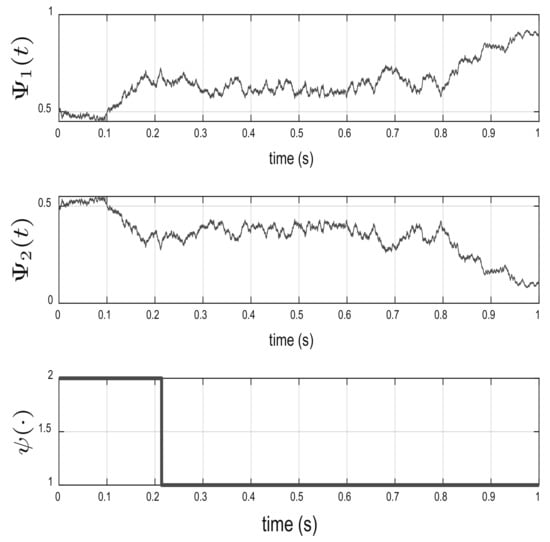
Figure 1. Wonham filter for the $\alpha$-discounted LQR.

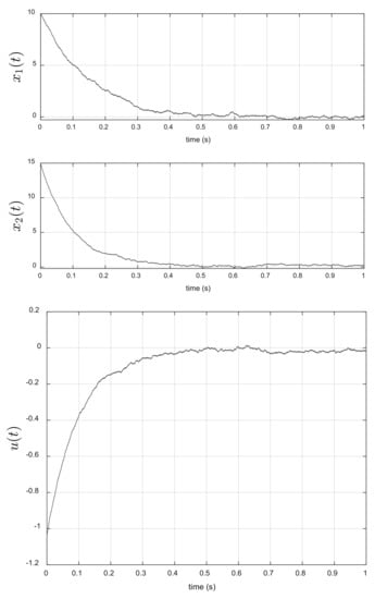
Figure 2. Asymptotic behavior of the state of dynamic system (top) and optimal control $\alpha$-discount LQR (bottom).

6. Application 2: Average LQR: Modeling of a Quarter-Car Suspension

In this section, the basic quarter-car suspension model analyzed in [27] is considered, see Figure 3. The parameters are: the sprung mass ($m_s$), the unsprung mass ($m_u$), the suspension spring constant ($k_s$), and the tire spring constant (k). Let $z_s,z_u$, and $z_r$ be the vertical displacements of the sprung mass, the unsprung mass, and the road profile, respectively. The equations of motion for this model are given by:

$$\begin{array}{ccc}\hfill m_s{z}_s^{″}\left(t\right)& =& -k_s(z_s\left(t\right)-z_u\left(t\right))-u\left(t\right),\hfill \end{array}$$

(46)

$$\begin{array}{ccc}\hfill m_u{z}_u^{″}\left(t\right)& =& k_s(z_s\left(t\right)-z_u\left(t\right))-k(z_u\left(t\right)-z_r\left(t\right))+u\left(t\right).\hfill \end{array}$$

(47)

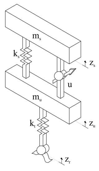
Figure 3. Schematic of a quarter-car suspension.

Now, defining $x_1\left(t\right)=z_s^{{}^{\prime }}\left(t\right)$, $x_2\left(t\right)=z_u^{{}^{\prime }}\left(t\right)$, $x_3\left(t\right)=z_s\left(t\right)-z_u\left(t\right)$, and $x_4\left(t\right)=z_u\left(t\right)-z_r$, the equations of motion (46) and (47) can be expressed in matrix form as:

$$dx\left(t\right)=(Ax\left(t\right)+Bu\left(t\right))dt+C_{1}d{z}_r\left(t\right)$$

(48)

where $dx\left(t\right)=\left[\begin{array}{c}d{x}_1\left(t\right)\\ d{x}_2\left(t\right)\\ d{x}_3\left(t\right)\\ d{x}_4\left(t\right)\end{array}\right],$ $A=\left[\begin{array}{cccc}0& 0& \frac{k_s}{m_s}& 0\\ 0& 0& \frac{k_s}{m_u}& \frac{k}{m_u}\\ 1& -1& 0& 0\\ 0& 1& 0& 0\end{array}\right],$ $B=\left[\begin{array}{c}\frac{1}{m_s}\\ \frac{1}{m_s}\\ 0\\ 0\end{array}\right],$ $C_1=\left[\begin{array}{c}0\\ 0\\ 0\\ -1\end{array}\right]$, and in the time domain, the road profile, $z_r\left(t\right)$, can be represented as the output of a linear first-order filter to white noise as follows:

$$d{z}_r\left(t\right)=-a\left(\psi \left(t\right)\right)V{z}_r\left(t\right)dt+{\sigma }_{2}d{W}_1\left(t\right),$$

where V is the vehicle speed (assumed constant), ${\sigma }_2$ is a positive constant, and a is the road roughness coefficient depending on the type of road. Here, we assume that a depends on a hidden Markov chain, that is, $a\left(\psi \right(t\left)\right)$ with $\psi \left(t\right)\in \{1,2\}.$ In our case, we consider that the dynamic system (48) evolves with additional white noise, that is:

$$dx\left(t\right)=(Ax\left(t\right)+Bu\left(t\right))dt+{\sigma }_{1}dW\left(t\right)+C_{1}d{z}_r\left(t\right)$$

(49)

The experts introduced the following performance index in order to trade off between the ride comfort and the handling while maintaining the constraint on suspension deflection:

$$\begin{array}{ccc}\hfill J(x,\Psi ,u)& =& \underset{T\to \infty }{lim}\frac{1}{T}{\mathbb{E}}^{x,\Psi ,u}\left[{\int }_0^T\right[c_1{\frac{d^2{z}_s}{d^{2}t}}^2+c_2{[z_1\left(t\right)-z_u\left(t\right)]}^2\hfill \\ & +& c_3{[z_u\left(t\right)-z_r\left(t\right)]}^2+c_{4}u{\left(t\right)}^2\left]dt\right]\hfill \end{array}$$

(50)

Defining $y:=\left[{\frac{d^2{z}_s}{d^{2}t}}^2,{[z_1\left(t\right)-z_u\left(t\right)]}^2,{[z_u\left(t\right)-z_r\left(t\right)]}^2\right],$ $C:=diag(c_1,c_2,c_3),$ and $R:=\left[c_4\right]$, we can rewrite (50) as:

$$\begin{array}{ccc}\hfill J(x,\Psi ,u)& =& \underset{T\to \infty }{lim}\frac{1}{T}{\mathbb{E}}^{x,\Psi ,u}\left[{\int }_0^{T}yC{y}^T+u^T\left(t\right)Ru\left(t\right)dt\right]\hfill \end{array}$$

(51)

Now, from the equations of motion in (46) and (47), note that $y=Mx+Nu$ with $M=\left[\begin{array}{cccc}0& 0& \frac{k_s}{m_s}& 0\\ 0& 0& 1& 0\\ 0& 0& 0& 1\end{array}\right],$ and $N=\left[\begin{array}{c}-\frac{1}{m_s}\\ 0\\ 0\end{array}\right].$ Thus, replacing this matrix form of y in (51) we can rewrite (50) again as:

$$\begin{array}{ccc}\hfill J(x,\Psi ,u)& =& \underset{T\to \infty }{lim}\frac{1}{T}{\mathbb{E}}^{x,\Psi ,u}\left[{\int }_0^T(x^T{Q}_{1}x+2x^T{Q}_{2}u+u^T{R}_{1}u)dt\right]\hfill \end{array}$$

(52)

where $Q_1=M^{T}CM$, $Q_2=M^{T}CN$, $R_1=N^{T}CN+R$.

The optimal control problem (OCP). The OCP in this application consists of finding $u^{*}\in U$ such that it minimizes the performance index (52) considering that the dynamic system evolves according to the stochastic differential Equation (49).

In the dynamic programming technique, we need the infinitesimal generator ${\mathcal{L}}^u$ of the process $\left(x\right(t),\Psi (t\left)\right)$ applied to $v(x,\Psi ,z_r)\in C^{2,2,2}({\mathbb{R}}^n\times S_N\times \mathbb{R})$; in this case, this generator is:

$$\begin{array}{ccc}\hfill {\mathcal{L}}^{u}vs.(x,\Psi ,z_r)=-a(\Psi \left(t\right))v_{z_r}(x,\Psi ,z_r)& & \hfill \\ \hfill +(Ax+Bu)v_x(x,\Psi ,z_r)& & \hfill \\ \hfill +{\mathcal{Q}}^T\Psi v_{\Psi }\left(x,\Psi ,z_r\right)& & \hfill \\ \hfill +\frac{1}{2}Tr\left[{\sigma }_1{\sigma }_1^T\right]v_{xx}(x,\Psi ,z_r).& & \hfill \\ \hfill +\frac{1}{2}Tr\left[{\sigma }_2{\sigma }_2^T\right]v_{z_r{z}_r}(x,\Psi ,z_r)& & \hfill \\ \hfill +\frac{1}{2}{v}_{\Psi \Psi }\left(x,\Psi ,z_r\right)Tr\left[A_2\right]& \end{array}$$

(53)

where $A_2(\Psi \left(t\right))=[{\sigma }_0^{-1}\left(\mathrm{diag}\left(h\right)-h^T(\Psi \left(t\right))I_N\right)\Psi \left(t\right)]{[{\sigma }_0^{-1}\left(\mathrm{diag}\left(h\right)-h^T(\Psi \left(t\right))I_N\right)\Psi \left(t\right)]}^T$, whereas the Hamilton–Jacobi–Bellman Equation (or dynamic programming equation) associated with this problem is:

$$J=\underset{u\in U}{max}[x^T{Q}_{1}x+2x^T{Q}_{2}u+u^T{R}_{1}u+{\mathcal{L}}^{u}vs.(x,\Psi ,z_r)]\mathrm{for} \mathrm{all}(x,\Psi )\in {\mathbb{R}}^n\times S_N,$$

(54)

see [28] for more details.

Proposition 3.

Assume that$(x\left(t\right),z_r\left(t\right),\Psi \left(t\right))$evolves according to (49). Then, the control that minimizes the long-run cost (52) is:

$$f^{*}(x,\Psi ,z_r)=-R_1^{-1}{(Q_2^T+B^{T}K)}^{T}x\left(t\right),$$

(55)

whereas the corresponding function v that solves the HJB Equation (54) is given by:

$$v(x,\Psi ,z_r)=x^{T}Kx+g\left(z_r\right)+n(\Psi )$$

where K is a positive semi-definite matrix that satisfies the Ricatti differential equation

$$\begin{array}{ccc}\hfill K(A-B{R}_1^{-1}{Q}_2^T)+(A-B{R}_1^{-1}{Q}_2^T)K-KB{R}_1{B}^{T}P& & \hfill \\ \hfill (Q_1-Q_2{R}_1^{-1}{Q}_2^T)=0,& & \hfill \end{array}$$

(56)

and$g(·)\in C^2\left(\mathbb{R}\right)$satisfies the differential equation:

$$\begin{array}{c}\hfill a(\Psi )g^{\prime }\left(z_r\right)+\frac{1}{2}{\sigma }_2^2{g}^{″}\left(z_r\right)=0,\end{array}$$

(57)

and$n(·)\in {\mathcal{C}}^2\left(S_N\right)$satisfies the partial differential equation:

$$\begin{array}{c}\hfill Q^T\Psi n^{\prime }(\Psi \left(t\right))+\frac{1}{2}Tr\left[A_2\right]n^{″}(\Psi )=0,\end{array}$$

(58)

where$A_2$is as in (41) and$n{}^{\prime }$ and $n{}^{″}$ denote the gradient and the Hessian of the n, respectively. The optimal cost is given by:

$$J=Tr\left[{\sigma }_1{\sigma }_1^T\right]K=J^{*}(x,\Psi )=\underset{u\in U}{min}J(x,\Psi ,u).$$

 Proof.

The HJB-equation for the partially observed LQR optimal control problem with $\left(x\right(t),\Psi (t\left)\right)$ evolves according to (49) and finite cost (52) is (54), where ${\mathcal{L}}^{u}v(t,x,w,\Psi )$ is the infinitesimal generator given in (53). We are looking for a candidate solution $h\in {\mathcal{C}}^{2,2,2}({\mathbb{R}}^n\times S_N\times \mathbb{R})$ to (54) in the form:

$$v(x,\Psi ,z_r)=x^{T}Kx+g\left(z_r\right)+n(\Psi ),$$

(59)

for some continuous functions $g(·)\in {\mathcal{C}}^2\left(\mathbb{R}\right)$, $h(·)\in {\mathcal{C}}^2\left(S_N\right)$ and K a positive semi-definite matrix. We assume that $g^{″}\left(z_r\right)>0$ for all $z_r\in \mathbb{R}$ and $n^{″}(\Psi )$ is positive definite, so that the function $(x,\Psi ,z_r)\to v(x,\Psi ,z_r)$ is convex.

Now, the function $u\in U\to 2x^T{Q}_{2}u+u^T{R}_{1}u+Bu{v}_x$ is strictly convex on the compact set U, and thus, attains its minimum at:

$$f^{*}(x,\Psi ,z_r)=-\frac{1}{2}{R}^{-1}[-2x^T{Q}_2-B{h}_x]=-R_1^{-1}{(Q_2^T+B^{T}K)}^{T}x\left(t\right).$$

(60)

Inserting $f^{*}(x,\Psi ,z_r)$ and the partial derivatives of v with respect to x, $z_r$, and $\Psi$ in the HJB-Equation (54), we obtain:

$$\begin{array}{ccc}\hfill J& =& x^T{Q}_{1}x+2x^T{Q}_2(-R_1^{-1}{(Q_2^T+B^{T}K)}^{T}x)\hfill \\ & +& {(-R_1^{-1}{(Q_2^T+B^{T}K)}^{T}x)}^T{R}_1(-R_1^{-1}{(Q_2^T+B^{T}K)}^{T}x)\hfill \\ & -& a(\Psi \left(t\right))g^{\prime }\left(z_r\right)+(Ax+B(-R_1^{-1}{(Q_2^T+B^{T}K)}^{T}x))2Kx+{\mathcal{Q}}^T\Psi h^{{}^{\prime }}(\Psi )++Tr\left[{\sigma }_1{\sigma }_1^T\right]K\hfill \\ & +& \frac{1}{2}Tr\left[{\sigma }_2{\sigma }_2^T\right]g^{{}^{″}}\left(z_r\right)+\frac{1}{2}{h}^{{}^{″}}(\Psi )Tr\left[A_2\right].\hfill \end{array}$$

(61)

For equality (61) to hold, it is necessary that the functions g and h satisfy (57) and (58), respectively, and the matrix K satisfies the Ricatti differential Equation (56), whereas the constant $J=Tr\left[{\sigma }_1{\sigma }_1^T\right]K$. Finally, from the Theorem 1, it follows that $f^{*}$ is an optimal Markovian control and the value function $J_T^{*}(t,x,w,\Psi )$ is equal to (59). That is:

$$J^{*}(x,\Psi )=\underset{u\in U}{min}J(x,\Psi ,u)=J=Tr\left[{\sigma }_1{\sigma }_1^T\right]K.$$

□

Simulation results. To solve the Wonhan filter, we use the numerical method given in ([18], Section 8.4), considering that the Markov chain $\psi \left(t\right)$ has two states that can only be observed through $dy\left(t\right)=h\left(\psi \left(t\right)\right)+{\sigma }_{0}dB\left(t\right)$. The following data were used: ${\sigma }_1=1$, ${\sigma }_2=1$, ${\sigma }_0=1$, $\alpha =0.01$, $a\left(1\right)=0.03$, $a\left(2\right)=0.015$, ${\Psi }_1\left(0\right)=0.5$, ${\Psi }_2\left(0\right)=0.5$, $R=1.0239$ × ${10}^{-5}$, $h\left(1\right)=-1$, $h\left(2\right)=0.5$, $m_s=329$ kg, $m_u=51$ kg, $k_s=4300$ N/m, $k=210,000$ N/m, $V=20$ m/s, $c_1=1$, $c_2=c_3=1\times {10}^5$, $c_4=1\times {10}^{-6}$ and:

$$Q=\left[\begin{array}{cc}-0.3& 0.3\\ 0.5& -0.5\end{array}\right].$$

The solution of the Wonham filter equation and the states of the hidden Markov chain $\psi \left(t\right)$ are shown in Figure 4. As can be noted, in $t=1$ s, ${\Psi }_1\left(1\right)=\mathbb{P}(\psi \left(t\right)=1|y\left(s\right),0\le s\le 1)\ge {\Psi }_2\left(1\right)$, implying that the Markov Chain with a probability greater than $0.5$ is in state 1 at $t=1$.

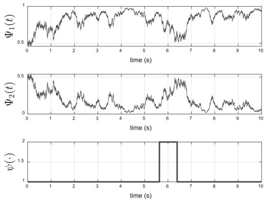
Figure 4. Wonham filter and hidden Markov chain (in t = 1 s).

The asymptotic behavior of the optimal control (55) is given in Figure 5 (bottom). It is interesting to note that this control minimizes the magnitude of the sprung mass velocity, $x_1=z_s^{{}^{\prime }}$ and unsprung mass velocity, $x_2=z_u^{{}^{\prime }}$ after $t=9$ s, see Figure 5 (top). This behavior implies that the magnitude of the sprung mass acceleration, $x_1=z_s^{{}^{″}}$ and unsprung mass acceleration $x_2=z_u^{{}^{\prime }}$ are also minimized, considering that the stochastic differential equation that models the road profile depends on a hidden Markov chain. These results agree with the obtained by authors in [27]. These authors mentioned that two important objectives of a suspension system are ride comfort and handling performance. The ride comfort requires that the car body be isolated from road disturbances as much as possible to provide a good feeling for passengers. In practice, we are looking to minimize the acceleration of the sprung mass.

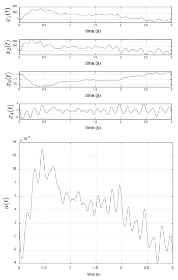
Figure 5. Asymptotic behavior of the state of dynamic system (top) and optimal control (bottom).

7. Application 3: Optimal Control of a Vehicle Active Suspension System with Damp

The model analyzed in this subsection is given in [29]. In this application, a damp $b_s$ is added to the quarter-car suspension given in Section 6, see Figure 6. The parameters in Figure 6 are: the sprung mass ($m_s$), the unsprung mass ($m_u$), the suspension spring constant ($k_s$), and the tire spring constant (k). Let $z_s,z_u$, and r be the vertical displacements of the sprung mass, the unsprung mass, and the road disturbance, respectively. The equations of motion are given by:

$$\begin{array}{ccc}\hfill m_s{z}_s^{{}^{″}}\left(t\right)& =& -k_s(z_s\left(t\right)-z_u\left(t\right))+b_s(z_u^{\prime }-z_s^{\prime })+u\left(t\right),\hfill \end{array}$$

(62)

$$\begin{array}{ccc}\hfill m_u{z}_u^{{}^{″}}\left(t\right)& =& k_s(z_s\left(t\right)-z_u\left(t\right))-k(r\left(t\right)-z_u\left(t\right))-b_s(z_u^{\prime }-z_s^{\prime })-u\left(t\right).\hfill \end{array}$$

(63)

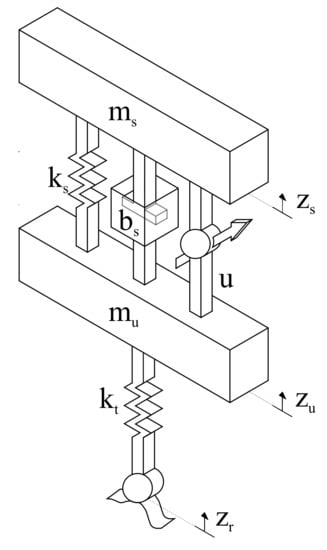
Figure 6. Quarter vehicle model of active suspension system.

Now, defining $x_1\left(t\right)=z_s\left(t\right)$, $x_2\left(t\right)=z_u\left(t\right)$, $x_3\left(t\right)=z_s^{\prime }\left(t\right)$, and $x_4\left(t\right)=z_u^{\prime }\left(t\right)$, the equations of motion in (62) and (63) can be expressed in matrix form as:

$$dx\left(t\right)=\left(Ax\right(t)+Bu(t\left)\right)dt+Fr\left(t\right)$$

(64)

where $dx\left(t\right)=\left[\begin{array}{c}d{x}_1\left(t\right)\\ d{x}_2\left(t\right)\\ d{x}_3\left(t\right)\\ d{x}_4\left(t\right)\end{array}\right],$ $A=\left[\begin{array}{cccc}0& 0& 1& 0\\ 0& 0& 0& 1\\ -\frac{k_s}{m_s}& \frac{k_s}{m_s}& -\frac{k_s}{m_s}& \frac{k_s}{m_s}\\ \frac{k_s}{m_u}& -\frac{(k_s+k)}{m_u}& \frac{b_s}{m_u}& -\frac{b_s}{m_u}\end{array}\right],$ $B=\left[\begin{array}{c}0\\ 0\\ \frac{1}{m_s}\\ -\frac{1}{m_u}\end{array}\right],$ $F=\left[\begin{array}{c}0\\ 0\\ 0\\ \frac{k}{m_u}\end{array}\right]$, and we assume that the road profile $r\left(t\right)$ is represented by a function with hidden Markovian switchings:

$$r\left(t\right)=\left\{\begin{array}{c}a\left(\psi \left(t\right)\right)\{1-cos\left(8\pi t\right)\},{\tau }_p\le t\le {\tau }_{p+1}\\ 0otherwise\end{array}\right.$$

(65)

where $a\left(1\right)=0.05$ (road bump height is 10 cm), $a\left(2\right)=0.025$ (road bump height is 16 cm), and ${\tau }_p$, $p=1,2,\dots$ are the random jump times of $\psi \left(t\right)$. In our case, we consider that the dynamic system (64) evolves with additional white noise, that is:

$$dx\left(t\right)=\left(Ax\right(t)+Bu(t)+Fr(t\left)\right)dt+\sigma dW\left(t\right)$$

(66)

and we wish to minimize the discounted expected cost:

$$V_{\alpha }(x,\Psi ,u):={\mathbb{E}}_{x,\Psi }^u\left[{\int }_0^{\infty }{e}^{-\alpha s}\{x^T\left(s\right)Dx\left(s\right)+u^T\left(s\right)Ru\left(s\right)\}ds\right],$$

subject to (66) and (65). Considering the infinitesimal generator given in (53) with $z_r\left(t\right)\equiv r\left(t\right)$ and the Hamilton–Jacobi–Bellman equation associated as the following problem:

$$\alpha v(x,\Psi )=\underset{u\in U}{max}[x^{T}Dx+u^T{R}_{1}u+{\mathcal{L}}^{u}vs.(x,\Psi ,r)]forall(x,\Psi )\in {\mathbb{R}}^n\times S_N,$$

similar arguments to these given in Section 5 and Section 6 allow us to find the optimal control $f^{*}$ and the value function $v^{*}$ for this setting. In fact:

$$v^{*}(x,\Psi )=x^{T}Kx+n(\Psi )+g\left(r\right)+c,$$

where $n:S_N\to \mathbb{R}$ is a twice differentiable continuous function, c is a constant, $g:\mathbb{R}\to \mathbb{R}$ is a twice differentiable continuous function, and K is a positive definite matrix. Inserting the derivative of $v(x,\Psi )$ in (43), we get the optimal control:

$$f^{*}(x,\Psi )=-{\overline{R}}^{-1}(\Psi )B^T{K}^{T}x,$$

(67)

where the matrix K satisfies the algebraic Riccati equation:

$$\begin{array}{cc}\hfill A^{T}K+KA-KB{R}^{-1}{B}^{T}K+D-\alpha K=0,& \end{array}$$

$$c=Tr\left[\sigma {\sigma }^{T}K\right]/\alpha ,$$

the function $g\in {\mathcal{C}}^2\left(\mathbb{R}\right)$ satisfies the differential equation:

$$\begin{array}{c}\hfill a(\Psi \left(t\right))g^{\prime }\left(r\right)+\alpha g\left(r\right)=0,\end{array}$$

and $n(·)\in {\mathcal{C}}^2\left(S_N\right)$ satisfies the partial differential equation:

$$\begin{array}{c}\hfill Q^T\Psi \left(t\right)n^{\prime }(\Psi \left(t\right))+\frac{1}{2}Tr\left[A_2\right]n^{″}(\Psi \left(t\right))-\alpha n(\Psi \left(t\right)))I_4=0,\forall \Psi \left(t\right)\in S_N,\end{array}$$

where $A_2$ is as in (42), $I_4$ is the identity matrix of $4\times 4$, and $n^{{}^{\prime }}$ and $n^{{}^{″}}$ are the gradient and the Hessian of the n, respectively.

Simulation results. To solve the Wonhan filter, we use the numerical method given in ([18], Section 8.4) considering that the Markov chain $\psi \left(t\right)$ has two states and that can be only observed through $dy\left(t\right)=h\left(\psi \left(t\right)\right)+{\sigma }_{0}dB\left(t\right)$. The following data were used: $\sigma =1$, ${\sigma }_0=1$, $\alpha =0.01$, $a\left(1\right)=0.05$, $a\left(2\right)=0.08$, ${\Psi }_1\left(0\right)=0.4$, ${\Psi }_2\left(0\right)=0.6$, $h\left(1\right)=1,h\left(2\right)=2$, $R=1.0239\times {10}^{-5}$, $m_s=300$ kg, $m_u=60$ kg, $k_s=1600$ N/m, $k=190,000$ N/m, $b_s=1000$ N/m, and:

$$Q=\left[\begin{array}{cc}-0.2& 0.2\\ 0.4& -0.4\end{array}\right].$$

Figure 7 shows the solution of the Wonham filter equation and the states of the hidden Markov chain $\psi \left(t\right)$. As can be seen, in the time interval $[2,4]$, ${\Psi }_1\left(1\right)=\mathbb{P}(\psi \left(t\right)=1|y\left(s\right),0\le s\le 1)\ge {\Psi }_2\left(1\right)$, implying that the Markov chain with a probability greater than $0.5$ is in state 1.

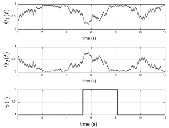
Figure 7. Wonham filter and hidden Markov chain (time interval [2, 4]).

The asymptotic behavior of the optimal control (67) is given in Figure 8 (bottom). It is interesting to note that this control minimizes the magnitude of the sprung mass, $x_1=z_s$, and unsprung mass, $x_2=z_u$, al well as their velocities, $x_3=z_s^{{}^{\prime }}$ and $x_4=z_u^{{}^{\prime }}$, after $t=12$ s, see Figure 8 (top).

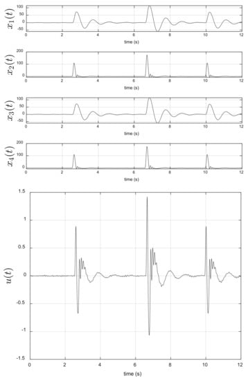
Figure 8. Asymptotic behavior of the state of the dynamic system (top) and optimal control (bottom).

8. Application 4: Optimal Pollution Control with Average Payoff

The application studies the pollution accumulation incurred by the consumption of a certain product, such as gas or petroleum, see [30]. The stock of pollution $x(·)$ is governed by the controlled diffusion process:

$$\mathrm{d}x\left(t\right)=\left[u\right(t)-\eta (\psi \left(t\right)\left)x\right(t\left)\right]\mathrm{d}t+k\mathrm{d}W\left(t\right),x\left(0\right)=x>0,$$

(68)

where $u\left(t\right)$ represents the pollution flow generated by an entity due to the consumption of the product, $\eta \left(\psi \right(t\left)\right)$ represents the decay rate of pollution, chosen at each time by nature, and k is a positive constant. We shall assume that $u\left(t\right)\in U=[0,\gamma ]$ is bounded and the parameter $\gamma$ represents the consumption/production restriction. Let $\psi \left(t\right)$ be a Markov chain with two states $E=\{1,2\}$ and a generator Q given by:

$$\left(\begin{array}{cc}{q}_{11}& q_{12}\\ q_{21}& q_{22}\end{array}\right)=\left(\begin{array}{cc}-{\lambda }_0& {\lambda }_0\\ {\lambda }_1& -{\lambda }_1\end{array}\right).$$

The reward rate $r:[0,\infty )\times E\times U\to \mathbb{R}$ in this example represents the social welfare and is defined as:

$$r(x,i,u):=F\left(u\right)-a\left(i\right)x,\forall (x,i,u)\in [0,\infty )\times E\times U,$$

(69)

where $F\in C^2\left(0,\infty \right)\cap C(0,\infty )$ and $D=a\left(i\right)x\in C\left(\right[0,\infty )\times E)$ is the social utility of the consumption u and the social disutility of the pollution $(x,i)$, respectively. We assume that the function F in (69) satisfies:

$$\left\{\begin{array}{c}{F}^{\prime }\left(u\right)>0,F^{″}\left(u\right)<0,\hfill \\ F^{\prime }(\infty )=F\left(0\right)=0,F^{\prime }(0+)=F(\infty )=\infty ,\hfill \end{array}\right.$$

Clearly, (68) is a liner stochastic differential equation, and satisfies Assumption 1.

Now, we define the Banach space ${\mathcal{B}}_w(\mathbb{R}\times E)$ and use $w(x,i):=x+i$, $w(x,\Psi )={\sum }_{i=1}^2{\Psi }_{i}w(x.i)={\Psi }_1(x+1)+{\Psi }_2(x+2)=x+(1-{\Psi }_1)$. Hence, ${lim}_{x\to +\infty }w(x,\Psi )=+\infty$ and Assumption 2i holds. On the other hand, since the utility function $F(·)$ is continuous on the compact interval $U=[0,\gamma ]$, then:

$$|r(x,i,u)|=|F\left(u\right)-a\left(i\right)x|\le (\underset{u\in [0,\gamma ]}{max}F\left(u\right)+\underset{i\in \{1,2\}}{max}a\left(i\right))(x+i)=Mw(x,i)$$

where $M:={max}_{u\in [0,\gamma ]}F\left(u\right)+{max}_{i\in \{1,2\}}a\left(i\right)$; thus, Assumption 3 holds. Note that:

$${\mathcal{L}}^{u,\Psi }w(x,\Psi )=u-\eta \left(i\right)x-{\lambda }_0{\Psi }_1+{\lambda }_1(1-{\Psi }_1),\mathrm{for} \mathrm{all}x>0.$$

Thus, taking $q:={max}_{i\in E}\eta \left(i\right)$ and $p:={max}_{u\in [0,\gamma ]}u-({\lambda }_0-{\lambda }_1){\Psi }_1$ we obtain:

$${\mathcal{L}}^{u}w(x,\Psi )\le -pw(x,\Psi )+q\mathrm{for} \mathrm{all}x>0.$$

Therefore, Assumption 2(ii) holds. It can be proven that the process (68) satisfies Assumption 2.6 in [1]; thus, by ([1], Theorem 2.8), $x\left(t\right)$ is exponentially ergodic (Assumption 4). In this application, we seek a policy u that maximizes the long-run average welfare $J(x,i,f)$:

$$J(x,i,u):=\underset{T\to \infty }{lim\; inf}\frac{1}{T}{\mathbb{E}}_{x,i}^u\left[{\int }_0^T[F\left(u\right)-a\left(i\right)x]\mathrm{d}t\right].$$

We propose $v(x,\Psi )=v\left(x\right)+h(\Psi )$, where $v\in C^2(\mathbb{R}\times E)\cap {\mathcal{B}}_w(\mathbb{R}\times E)$ and $h\in C^2\left(S_N\right)$ as a solution that verify the HJB Equation (27) associated with this pollution control problem. Simple calculations allow us to conclude that the policy on consumption/pollution takes the form:

$$u:=f(x,\Psi )=\left\{\begin{array}{cc}I(-v^{\prime }\left(x\right))& if{F}^{\prime }\left(\gamma \right)<-v^{\prime }\left(x\right),\\ \gamma & if{F}^{\prime }\left(\gamma \right)\ge -v^{\prime }\left(x\right).\end{array}\right.$$

where $I(-v^{\prime }\left(x\right))$ is the inverse function of derivative $F^{\prime }$, $f\in \mathbb{F}$.

9. Concluding Remarks

Under hypotheses such as uniform ellipticity in Assumption 1c, the Lyapunov-like conditions in Assumption 2, and the w-exponential ergodicity in (4) for the average criterion, this work shows the existence of optimal controls for the control problems with discounted and average payoffs, where the dynamic system evolves according to switching diffusion with hidden states. To conclude, we conjecture that the results obtained in this work still hold (with obvious changes) if the hidden Markov chain ($\psi$) in (1) is replaced with any other diffusion process. Furthermore, these results can be extended to constrained and unconstrained nonzero-sum stochastic differential games with additive structures, which will allow us to model a larger class of practical systems. This will be a topic in future works.

References

- Escobedo-Trujillo, B.A.; Hernández-Lerma, O. Overtaking optimality for controlled Markov-modulated diffusions. J. Optim. 2011, 61, 1405–1426. [Google Scholar] [CrossRef]
- Borkar, V.S. The value function in ergodic control of diffusion processes with partial observations. Stoch. Stoch. Rep. 1999, 67, 255–266. [Google Scholar] [CrossRef]
- Borkar, V.S. Dynamic programming for ergodic control with partial observations. Stoch. Process. Their Appl. 2003, 103, 293–310. [Google Scholar] [CrossRef]
- Rieder, U.; Bäuerle, N. Portfolio optimization with unobservable Markov-modulated drift Process. J. Appl. Probab. 2005, 362–378. [Google Scholar] [CrossRef] [Green Version]
- Tran, K. Optimal exploitation for hybrid systems of renewable resources under partial observation. Nonlinear Anal. Hybrid Syst. 2021, 40, 101013. [Google Scholar] [CrossRef]
- Tran, K.; Yin, G. Stochastic competitive Lotka–Volterra ecosystems under partial observation: Feedback controls for permanence and extinction. J. Frankl. Inst. 2014, 351, 4039–4064. [Google Scholar] [CrossRef]
- Mao, X.; Yuan, C. Stochastic Differential Equations with Markovian Switching; World Scientific Publishing Co.: London, UK, 2006; Available online: https://www.worldscientific.com/doi/pdf/10.1142/p473 (accessed on 20 March 2022). [CrossRef]
- Yin, G.G.; Zhu, C. Hybrid Switching Diffusions. In Stochastic Modelling and Applied Probability; Properties and Applications; Springer: New York, NY, USA, 2010; Volume 63, p. xviii+395. [Google Scholar] [CrossRef]
- Yin, G.; Mao, X.; Yuan, C.; Cao, D. Approximation methods for hybrid diffusion systems with state-dependent switching processes: Numerical algorithms and existence and uniqueness of solutions. SIAM J. Math. Anal. 2009, 41, 2335–2352. [Google Scholar] [CrossRef] [Green Version]
- Yu, L.; Zhang, Q.; Yin, G. Asset allocation for regime-switching market models under partial observation. Dynam. Syst. Appl. 2014, 23, 39–61. [Google Scholar]
- Ghosh, M.K.; Arapostathis, A.; Marcus, S.I. Optimal control of switching diffusions with application to flexible manufacturing systems. SIAM J. Control Optim. 1993, 31, 1183–1204. [Google Scholar] [CrossRef]
- Ghosh, M.K.; Marcus, S.I.; Arapostathis, A. Controlled switching diffusions as hybrid processes. In Proceedings of the International Hybrid Systems Workshop, New Brunswick, NJ, USA, 22–25 October 1995; Springer: Berlin/Heidelberg, Germany, 1995; pp. 64–75. [Google Scholar]
- Zhang, X.; Zhu, Z.; Yuan, C. Asymptotic stability of the time-changed stochastic delay differential equations with Markovian switching. Open Math. 2021, 19, 614–628. [Google Scholar] [CrossRef]
- Zhu, C.; Yin, G. Asymptotic properties of hybrid diffusion systems. SIAM J. Control Optim. 2007, 46, 1155–1179. [Google Scholar] [CrossRef]
- Wonham, W.M. Some applications of stochastic differential equations to optimal nonlinear filtering. J. SIAM Control Ser. A 1965, 2, 347–369. [Google Scholar] [CrossRef]
- Elliott, R.J.; Aggoun, L.; Moore, J.B. Hidden Markov Models: Estimation and Control; Springer: Berlin/Heidelberg, Germany, 1995. [Google Scholar]
- Cohen, S.N.; Elliott, R.J. Stochastic Calculus and Applications, 2nd ed.; Probability and Its Applications; Springer: Cham, Switzerland, 2015; p. xxiii+666. [Google Scholar] [CrossRef]
- Yin, G.; Zhang, Q. Discrete-Time Markov Chains: Two-Time-Scale Methods and Applications; Stochastic Modelling and Applied Probability; Springer: New York, NY, USA, 2006. [Google Scholar]
- Yin, G.G.; Zhu, C. Hybrid Switching Diffusions: Properties and Applications; Springer Science & Business Media: Berlin/Heidelberg, Germany, 2009; Volume 63. [Google Scholar]
- Protter, P.E. Stochastic integration and differential equations. In Stochastic Modelling and Applied Probability, 2nd ed.; Version 2.1, Corrected Third Printing; Springer: Berlin/Heidelberg, Germany, 2005; Volume 21, p. xiv+419. [Google Scholar] [CrossRef]
- Chigansky, P. An ergodic theorem for filtering with applications to stability. Syst. Control Lett. 2006, 55, 908–917. [Google Scholar] [CrossRef]
- Kunita, H. Asymptotic behavior of the nonlinear filtering errors of Markov processes. J. Multivar. Anal. 1971, 1, 365–393. [Google Scholar] [CrossRef] [Green Version]
- Lu, X.; Yin, G.; Guo, X. Infinite Horizon Controlled Diffusions with Randomly Varying and State-Dependent Discount Cost Rates. J. Optim. Theory Appl. 2017, 172, 535–553. [Google Scholar] [CrossRef]
- Ghosh, M.K.; Arapostathis, A.; Marcus, S.I. Ergodic control of switching diffusions. SIAM J. Contr. Optim 1997, 35, 1962–1988. [Google Scholar] [CrossRef]
- SchÄl, M. Conditions for optimality and for the limit of n-stage optimal policies to be optimal. Z. Wahrs. Verw. Gerb. 1975, 32, 179–196. [Google Scholar] [CrossRef]
- Ghosh, M.K.; Marcus, S.I. Stochastic differential games with multiple modes. Stoch. Anal. Appl. 1998, 16, 91–105. [Google Scholar] [CrossRef]
- Nguyen, L.H.; Seonghun, P.; Turnip, A.; Hong, K.S. Application of LQR Control Theory to the Design of Modified Skyhook Control Gains for Semi-Active Suspension Systems. In Proceedings of the ICROS-SICE International Joint Conference 2009, Fukuoka, Japan, 18–21 August 2009; pp. 4698–4703. [Google Scholar]
- Escobedo-Trujillo, B.; Garrido-Meléndez, J. Stochastic LQR optimal control with white and colored noise: Dynamic programming technique. Rev. Mex. Ing. QuÍmica 2021, 20, 1111–1127. [Google Scholar] [CrossRef]
- Maurya, V.K.; Bhangal, N.S. Optimal Control of Vehicle Active Suspension System. J. Autom. Control. Eng. 2018, 6, 1111–1127. [Google Scholar] [CrossRef]
- Kawaguchi, K.; Morimoto, H. Long-run average welfare in a pollution accumulation model. J. Econom. Dynam. Control 2007, 31, 703–720. [Google Scholar] [CrossRef]
Publisher’s Note: MDPI stays neutral with regard to jurisdictional claims in published maps and institutional affiliations. |
© 2022 by the authors. Licensee MDPI, Basel, Switzerland. This article is an open access article distributed under the terms and conditions of the Creative Commons Attribution (CC BY) license (https://creativecommons.org/licenses/by/4.0/).